Detailed Investigation of the Droplet Dynamics Parameters Produced by Artificially Induced Bag-Breakup Fragmentation

Abstract

This paper presents the results of detailed studies of the processes of droplet formation and its characteristics under conditions of artificially induction of a bag-breakup fragmentation event. A shadow imaging method was used in combination with the high-speed video filming of the side-view fragmentation process. Trajectories and ejection velocity characteristics of the formed droplets are determined by identifying particles in consecutive frames with combined use of Particle Imaging Velocimetry (PIV) and Particle Tracking Velocimetry (PTV). Based on the results of trajectory processing, the distributions of droplet velocities for the selected regions are obtained, and estimates of the ejection velocities at various heights are proposed.

1. Introduction

Sea spray is a typical element of the marine atmospheric boundary layer with important environmental effect. In many experimental and theoretical works, droplets are considered as one of the main factors affecting the exchange of momentum between the atmosphere and the ocean under hurricane conditions (see, for example, reviews [1,2]). Sea spray is considered as a significant factor affecting the air–sea fluxes at high winds and development of severe storms [3,4,5,6,7]. Air–sea interaction at extreme winds is of special interest now in connection with the problem of the sea surface drag reduction at wind speeds exceeding 30–35 m/s. This phenomenon, predicted by [3] and confirmed by a number of field [4,5] and laboratory [6,7] experiments, still waits its physical explanation. Several papers attributed the drag reduction to spume droplets-spray tearing off the crests of breaking waves [8,9] due to direct transfer of momentum by droplets moving in a turbulent boundary layer, which is proved to be more effective than the effect associated with the suppression of turbulent exchange due to stratification caused by the presence of laden droplets in the air [10]. For a quantitative description of the influence on the characteristics of the boundary layer from moving droplets in it, phenomenological models [8,9], approaches based on the use of Lagrangian stochastic models [11,12,13], as well as direct numerical simulation of an air-turbulent boundary layer above a rough surface in the presence of drops [14,15,16] were used. Regardless of the approach used, the obtained results strongly depended on the speed at which the droplets are ejected into the atmosphere. Thus, in [10,11], the ejection velocity was equated to the local air flow velocity. In turn, in [12], the ejection velocity was taken equal to the velocity of the water surface. Two different models of droplet ejection were used in [13,16], depending on the mechanism of the spray generation, namely, the spume droplet mechanism, by Koga [17], or bubble bursting, studied in [18]. Depending on the ejection velocity, the momentum exchange of the droplets with the air can either increase or decrease the surface drag coefficient of the air–water interface.

Recent studies of the air–water interaction at high wind [19,20] have shown that the dominant mechanism of spume droplet generation is concerned with the “bag-breakup” fragmentation of the air–water interface. Thus, in [20], the initial velocities of the droplets were equated to the velocities of the “bags” canopy edges before rupture, which were estimated from the processing of the high-speed video of the water surface from above. However, the top view images do not allow us to correctly estimate the vertical component of the ejection velocity and the height at which the drop is located from the surface.

The problems described above stimulated the present work, where the parameters of the dynamics of drops were studied, their trajectories were reconstructed, and the ejection velocities were estimated in a detailed study with an artificially generated bag-breakup event in a laboratory experiment. Section 1 of the paper describes the experiment, including the procedure for artificial initiation of this type of fragmentation event. Section 2 is devoted to the procedures for processing high-speed video to obtain information about the droplets formed. In Section 3, an analysis of the obtained distributions of the velocity of droplets at different heights is carried out. Finally, conclusions are given and directions for further research are identified.

2. Experimental Setup

A detailed study of the fragmentation events of the bag-breakup type with identification of the movement of individual drops under conditions of intensely breaking waves, caused by high wind speeds, is very difficult, even when using multi-angle high-speed video recording in laboratory experiments (see [20]). Therefore, we used a system for artificial generation of the bag-breakup event, which was developed (see [21]) for installation at the 10 m-long High-speed wind-wave flume (HSWWF) of the Institute of Applied Physics (IAP RAS). The scheme of the experimental setup with a cross-section of HSWWF is shown in Figure 1a. It should be mentioned that experimental setup was similar to that used in [7]. So, it was the same HSWWF (10 m long) which was inserted into a large water tank. The large tank was emptied. However, air flow tunnel of 40 cm by 40 cm was formed again by mounting solid plates on the level of water surface in previous experiments. A small reservoir (40 × 15 × 15 cm situated along the flume) was used, with water level flush with the surrounding bottom (solid plates). Most parts of the foam rubber and the nylon mesh, in particular, cover all water surface in this reservoir. Only area of about 3 × 3 cm was still open. Under this open area, a vertical nozzle (diameter 1cm on the 3 cm depth from water level) was located. It created a vertical underwater jet, causing a disturbance of the surface elevation which triggered a bag-breakup event to occur. This jet was automatically impulsively induced with special hydraulic–electronic system with remote control. The diameter of the nozzle was 6 mm, and bag-breakup fragmentation event induced in this reservoir.

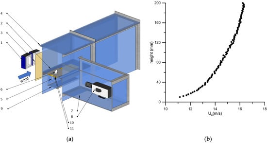
Figure 1. (a) The cross-section of the high-speed wind-wave flume with a system of artificial bag-breakup generation: 1—LED lights; 2—solid flat bottom; 3—opaque screen; 4—high-speed wind-wave flume; 5—nozzle; 6—bag-breakup; 7—semi-submerged box; 8—high-speed camera; 9—reservoir with water; 10—foam rubber in water; 11—nylon mesh; (b) Mean air flow profile in the point where artificial bag-breakup is induced.

More details about the HSWWF facility and the system for artificial bag-breakup generation can be found in [7,21].

The experiments were carried out for 40 Hz of the control frequency of the wind tunnel fan. Investigations were performed for one regime of air flow in wind tunnel corresponded to regular bag-breakup initialization. L-shaped Pitot gauge on scanning device was used to measure air flow velocity U_a profile at the working section with reservoir. It was measured from 1 to 20 cm height from the water level with vertical scanning speed of 1.1 mm/s. Five consecutive profiles were measured for subsequent averaging. The resulting velocity profile is shown in Figure 1b.

High-speed video filming in the shadowgraph visualization mode was applied to investigate the artificially induced bag-breakup fragmentation event in detail.

Side filming was realized using the high-resolution high-speed camera (NAC Memrecam HX-3) with opposite illumination source of two 300 W LED lights through vertical diffusing screen. The frame resolution of 2560 × 960 px and resolution of 63 μm/px provide total size of the imaging area of 161 × 60 mm. This allowed us to capture full evolution of the bag-breakup process. The recording was carried out at speed of 3990 fps and exposure time of 20 µs. The length of recording is 700 frames (175 ms). The record was interrupted at the moment the last droplets left the imaging area. At the moment the last droplet left the imaging area, the recording was stopped.

High-speed video of the artificially induced bag-breakup process (Figure 2a) showed that its behavior is close to what was previously observed for bag-breakup in laboratory conditions on the wavy surface of the water. The stages included: canopy formation, and rupture of its film, which leads to the formation of small droplets and subsequent rim fragmentation into large drops.

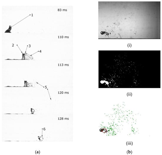
Figure 2. (a) Five sequent images obtained from the side of the bag-breakup for wind speed U₁₀ = 21.8 m/s. 1—initial disturbance; 2—rim; 3—film; 4—film rupture; 5—film drops; 6—rim drops. Full image width 161 mm; (b) Image processing sequence for a frame at 113 ms after film rupture, U₁₀ = 21.8 m/s, 81 mm downwind the initial disturbance, 33 mm above surface. (i) initial image; (ii) binary image with marked droplet areas; (iii) detected droplets (green circles—detected droplets; red—deleted image of rim).

3. Description of the Procedure of Image Processing

Specially developed software, which includes algorithms of droplet edge detection, PIV processing and PTV method, is used to obtain quantitative data on the characteristics and dynamics of droplets formed during both stages of bag-breakup fragmentation. The image processing contained two main stages: (1) droplet detection, (2) droplet tracking.

The image processing sequence to detect the position of all visible droplets in each frame of the record is illustrated in Figure 2b, for a fragment of one frame. The algorithm for imaged segmentation used in this investigation is similar to what was described in detail in [22] for water surface detection within laser measurements. This method includes several steps: calculation and subtraction of the background, edge detection with Sobel operator, and morphological operations to remove noise and fill closed areas. The main feature of this sequence is a logical ‘or’ performed with binary of initial image. Keeping the noise low allowed us to not lose small droplets. Finally, the positions and shapes of all isolated regions were estimated. The area of the image of the canopy and rim were obtained in a similar way but with different thresholds. Then, these images were deleted on each frame to prevent its influence on the results of droplets detection. The algorithm can only detect droplets larger than 60 µm images captured from a side view, but the same algorithm can be used for smaller droplets using video with a higher resolution.

Data on the coordinates of each droplet on each frame were used to retrieve droplet trajectories with a specially developed algorithm. It was easier to separate trajectories when the density of droplets was lower, which is why we performed tracking backward in time from later to earlier frames. We tried to find an appropriate droplet on the previous frame in the vicinity of its assumed position going through the recording from the end to the beginning.

Two methods for estimation of assumed droplet position were used. The first (main) method is based on parabolic extrapolation for coordinates of four previously found points of current trajectory, assuming a constant acceleration. The second is based on the estimation of the droplet’s displacement interpolated from the velocity fields obtained by PIV processing of the sequent images. PIV is used as an auxiliary method, first of all, to obtain rough estimates of the droplet velocities and determine if there are some problems with extrapolation (for trajectories containing less than four known points). Custom PIV processing software, which was developed for the estimation of the air flow velocity field in [22], was also used in this work. Cross-correlation processing of the pair of sequent frames were used on the grid with interrogation windows 128 × 128 px and 50% overlapping. One-step iteration with three-point Gaussian interpolation of the peak of cross-correlation function was used. Displacements were obtained on a rectangular grid using maximum and minimum velocity thresholds, then using a two-dimensional median filter, and finally interpolating to the position of each droplet (Figure 3a). Thus, a rough estimate was obtained for the displacement of each drop between each frame.

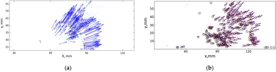
Figure 3. (a) Approximate velocity field obtained by PIV interpolated to position of each droplet (shown in circles)/(b) An example of a trajectory evaluation. Circles shows the search area near the assumed position. Blue straights are the previous four points of each trajectory. Red dots show the positions of all droplets on the frame.

Trajectory data, the last-found point of which is not more than three frames from a given one, is used for each frame. Thus, if positions have not been detected on one or two consecutive frames, the trajectory will still be constructed. The trajectory construction is terminated when there are no droplets in the vicinity of 20 pixels from the expected position or the radius of the droplet deemed to be the proper one is more than three times different from the previous one. If two trajectories find the same drop, the latter is assigned to the trajectory whose the distance to the supposed point of which is smaller. The use of four points for polynomial extrapolation allows us to take into account the scatter of the calculated coordinates. If it is too large, then the last-found point of the trajectory is neglected. An example of droplet tracking is shown in Figure 3b.

Postprocessing of trajectories consisted of filtering and combining split trajectories. Postprocessing of trajectories consisted of filtering and combining split trajectories. If the median displacement on the trajectory was less than 0.001 px/frame, or if the trajectory was shorter than 10 frames, it was rejected as noise. The algorithm can lose the droplet for several frames due to visible overlapping of the droplets. To address this problem, the standard deviation of the found positions and the polynomial extrapolation was calculated for each non-intersecting in time pair of trajectories. The trajectories were combined into one in case of low deviation. This combination is repeated until all split trajectories were combined. This algorithm enables assigning more than 75% of droplets to trajectories and retrieving more than 500 separate trajectories in the experiment.

4. Results of Image Processing and Droplets Ejection Velocity Estimation

Results of image processing are shown on Figure 4. On Figure 4a, dots indicate all positions of each droplet on each frame, and the color of the dots corresponded to the sequence in time (from blue to dark red). These points were collected in trajectories as shown on Figure 4b.

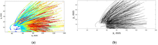
Figure 4. (a) Color from blue (first frame) to dark red (last frame) represented positions of all droplets on all frames in all frames one the record. (b) View on the all trajectories found in the entire video record.

The reconstructed trajectories of each drop were used to obtain the drop velocity distribution at certain heights. On the basis of these distributions, one can obtain estimates of the ejection velocities and heights. Obviously, the distribution parameters will strongly depend on the sizes of the search area. A rectangular area with a fixed horizontal size of 110 mm was chosen (to the left of the extreme position of the bag rim at the moment of membrane rupture, and to the frame edge on the right). The vertical size (further thickness) of the areas varied in the range from 0.6 mm to 18.8 mm. The vertical position of the areas (from 0 level to the middle of the area) varied from 35.2 to 56.5 mm. In this case, the minimum position of the lower horizontal boundary was higher than the maximum bag height observed in the experiment before its fragmentation began for all regions. In each case, a search was made for trajectories crossing a given area. It was carried out in two stages. First, all points of the trajectories located inside the area were selected. Then, all points of the trajectories were selected, the segments between which cross any of the boundaries of the area (in case the trajectory nevertheless crossed the area, but there were no points that fall inside the area).

For the points of each trajectory selected in this way and crossing the given area, the average position and average velocity were calculated. The results of finding segments of the trajectories and determining the average velocities are shown in Figure 5.

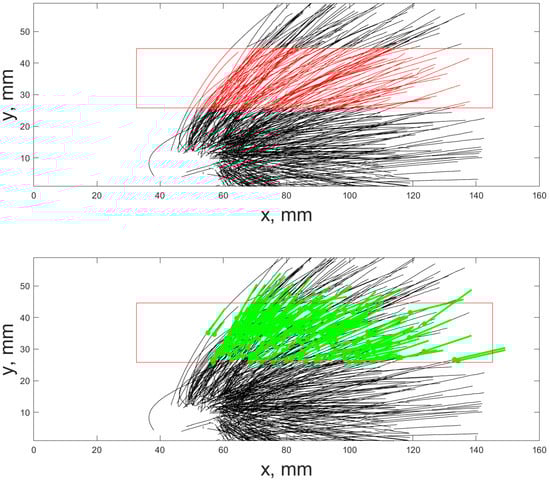
Figure 5. Illustrations of finding trajectories crossing the given search areas and determining average velocities. On the top image, segments of the trajectories crossing the search areas are marked in red. On the bottom image, the green straights corresponded mean velocity length, with denoting of the position (point) of its calculation.

The data obtained were used to construct normalized cumulative distributions of both velocity components (vertical and horizontal). They were approximated with a normal (Gaussian) distribution (for example, see Figure 6):

$$f=\frac{1}{2}\left(1+erf\left(\frac{x-\mu }{\sqrt{2{\sigma }^2}}\right)\right),$$

(1)

where µ is the mean, and σ is the dispersion.

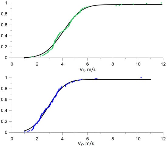
Figure 6. Example of the resulting cumulative distributions for the horizontal (green symbols) and vertical velocity (blue) components and their approximations by Gaussian distribution functions (1). Area of 18.8 mm thickness and position of 35.2 mm.

The mean values of the horizontal and vertical velocity components obtained from the approximations were plotted for each area depending on its position (see Figure 7).

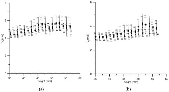
Figure 7. Dependence of the mean value, determined by approximations of the Gaussian distribution function, on the position of the droplet velocity determination region (a) for the horizontal component (b) of the vertical component. The symbols correspond to different thickness of the observation area: circle—0.6 mm; rectangle—1.3 mm; triangle—3.1 mm; rhombus—6.3 mm; cross—9.4; star—12.5; oblique cross—18.8 mm.

Both dependencies, for the horizontal and for the vertical components, show a growth behavior up to about a position of 47 mm, and then they can be considered constant, especially taking into account the size of the confidence intervals. It is this position that can be considered as an initial height for the ejection of droplets formed during the fragmentation event of the bag-breakup type. In this case, estimates of average velocities give about 3.5 m/s for the vertical component, and 5 m/s for the horizontal component. The dispersion for the first is approximately 1.6 m/s, and for the second, 2.3 m/s. Figure 1b shows that in the interval between 35 and 60 mm the flow velocity changes from 14.8 m/s to 15.6 m/s. It should be noted that the estimate of the vertical velocity significantly exceeds the dynamic velocity u* = 0.6 m/s determined based on the logarithmic approximation of the measured profile (see Figure 1b).

5. Conclusions

The developed algorithms for analyzing images of the processes of fragmentation (bag-breakup type) of a water surface blown by an air flow, obtained using high-speed video filming and shadowgraph visualization, made it possible to construct the trajectories of the droplets formed. These algorithms use a combination of PIV and the backward-in-time PTV method. Preliminary estimates show that the vertical velocities of drops typically hundreds of microns in size, which are generated during bag-breakup fragmentation, are unexpectedly high: the mean value of the vertical velocity is approximately 6u*, which is more than an order of magnitude higher than the estimate of the transverse droplet velocity obtained in [20] from top view images of the fragmentation process. This value also significantly exceeds the values of droplet ejection velocities, which were used in [11,12,13] in modeling the motion and heat transfer of droplets within the Lagrangian stochastic model, as well as in the framework of the phenomenological model [10]. It can be expected that using these high ejection velocities of droplets in the models will give higher values of the lifetime of large droplets in the atmospheric boundary layer than were predicted previously, and therefore, this provides more significant spray-mediated sensible and latent heat fluxes and also the enthalpy flux.

References

- Andreas, E.L.; Jones, K.F.; Fairall, C.W. Production velocity of sea spray droplets. J. Geophys. Res. 2010, 115, C12065. [Google Scholar] [CrossRef]
- Veron, F. Ocean spray. Annu. Rev. Fluid Mech. 2015, 39, 419–446. [Google Scholar] [CrossRef]
- Emanuel, K.A. Sensitivity of tropical cyclones to surface exchange coefficients and a revised steady-state model incorporating eye dynamics. J. Atmos. Sci. 1995, 52, 3969–3976. [Google Scholar] [CrossRef]
- Powell, M.D.; Vickery, P.J.; Reinhold, T.A. Reduced drag coefficient for high wind speeds in tropical cyclones. Nature 2003, 422, 279–283. [Google Scholar] [CrossRef] [PubMed]
- Bell, M.; Montgomery, M.T.; Emanuel, K.A. Air-sea enthalpy and momentum exchange at major hurricane wind speeds observed during CBLAST. J. Atmos. Sci. 2012, 69, 3197–3222. [Google Scholar] [CrossRef]
- Donelan, M.A.; Haus, B.K.; Reul, N.; Plant, W.J.; Stiassnie, M.; Graber, H.C.; Brown, O.B.; Saltzman, E.S. On the limiting aerodynamic roughness of the ocean in very strong winds. Geophys. Res. Lett. 2004, 31, L18306. [Google Scholar] [CrossRef]
- Troitskaya, Y.I.; Sergeev, D.A.; Kandaurov, A.A.; Baidakov, G.A.; Vdovin, M.A.; Kazakov, V.I. Laboratory and theoretical modeling of air-sea momentum transfer under severe wind conditions. J. Geophys. Res. 2012, 117, C00J21. [Google Scholar] [CrossRef]
- Kudryavtsev, V.N.; Makin, V.K. Impact of ocean spray on the dynamics of the marine atmospheric boundary layer. Bound. Layer Meteorol. 2011, 140, 383–410. [Google Scholar] [CrossRef]
- Andreas, E.L. Spray stress revisited. J. Phys. Oceanogr. 2004, 34, 1429–1440. [Google Scholar] [CrossRef]
- Kudryavtsev, V.N. On the effects of sea on the atmospheric boundary layer. J. Geophys. Res. 2006, 111, C07020. [Google Scholar] [CrossRef]
- Edson, J.B.; Fairall, C.W. Spray droplet modeling: 1. Lagrangian model simulation of the turbulent transport of evaporating droplets. J. Geophys. Res. 1994, 99, 25295–25311. [Google Scholar] [CrossRef]
- Mueller, J.A.; Veron, F. Impact of sea spray on air–sea fluxes. Part I: Results from stochastic simulations of sea spray drops over the ocean. J. Phys. Oceanogr. 2014, 44, 2817–2834. [Google Scholar]
- Troitskaya, Y.; Ezhova, E.V.; Soustova, I.A.; Zilitinkevich, S.S. On the effect of sea spray on the aerodynamic surface drag under severe winds. Ocean. Dyn. 2016, 66, 659–669. [Google Scholar] [CrossRef]
- Richter, D.H.; Sullivan, P.P. Sea surface drag and the role of spray. Geophys. Res. Lett. 2013, 40, 656–660. [Google Scholar] [CrossRef]
- Richter, D.H.; Sullivan, P.P. Momentum transfer in a turbulent, particle-laden Couette flow. Phys. Fluids 2013, 25, 053304. [Google Scholar] [CrossRef]
- Druzhinin, O.A.; Troitskaya, Y.; Zilitinkevich, S.S. The study of droplet-laden turbulent airflow over waved water surface by direct numerical simulation. J. Geophys. Res.Oceans 2017, 122, 1789–1807. [Google Scholar] [CrossRef]
- Koga, M. Direct production of droplets from breaking windwaves—Its observation by a multi-colored overlapping exposure photographing technique. Tellus 1981, 33, 552–563. [Google Scholar]
- Spiel, D.E. On the birth of jet drops from bubbles bursting on water surfaces. J. Geophys. Res. 1995, 100, 4995–5006. [Google Scholar] [CrossRef]
- Troitskaya, Y.; Kandaurov, A.; Ermakova, O.; Kozlov, D.; Sergeev, D.; Zilitinkevich, S. Bag-breakup fragmentation as the dominant mechanism of sea-spray production in high winds. Sci. Rep. 2017, 7, 1614. [Google Scholar] [CrossRef]
- Troitskaya, Y.I.; Kandaurov, A.; Ermakova, O.; Kozlov, D.; Sergeev, D.; Zilitinkevich, S. “Bag-breakup” spume droplet generation mechanism at hurricane wind. Part I. Spray generation function. J. Phys. Oceanogr. 2018, 48, 2167–2188. [Google Scholar] [CrossRef]
- Kandaurov, A.A.; Sergeev, D.A. A system of artificial initiation of the bag-breakup fragmentation for investigation of the spray generation processes during wind-wave interaction in laboratory experiments. At. Sprays 2021, 31, 21–33. [Google Scholar] [CrossRef]
- Kandaurov, A.A.; Troitskaya, Y.I.; Sergeev, D.A.; Vdovin, M.I.; Baidakov, G.A. Average velocity field of the air flow over the water surface in a laboratory modeling of storm and hurricane conditions in the ocean. Izv. Atmos. Ocean. Phys. 2014, 50, 399–410. [Google Scholar] [CrossRef]
Disclaimer/Publisher’s Note: The statements, opinions and data contained in all publications are solely those of the individual author(s) and contributor(s) and not of MDPI and/or the editor(s). MDPI and/or the editor(s) disclaim responsibility for any injury to people or property resulting from any ideas, methods, instructions or products referred to in the content. |
© 2022 by the authors. Licensee MDPI, Basel, Switzerland. This article is an open access article distributed under the terms and conditions of the Creative Commons Attribution (CC BY) license (https://creativecommons.org/licenses/by/4.0/).