Abstract
In this work, four radiators with different core geometries were tested using a wind tunnel. The values of the global heat transfer coefficient (UA = 5 ÷ 65 W/K) were measured depending on the flow of air and water. The obtained UA values correlate well with the data of sorption experiments described in the literature. The found correlations between the Nusselt and Reynolds numbers made it possible to propose an algorithm for ranging commercial air radiators for the use in adsorption heat transformers. It is shown that the use of a wind tunnel can serve as an effective tool for express assessment of the prospects of using air radiators for adsorption heat conversion without destroying radiators or their direct testing in a complex adsorption installation requiring vacuum maintenance.
1. Introduction
Due to the deteriorating environmental situation in the world, there is an increased interest in environmentally oriented adsorption heat transformation (AHT) systems for heating, cooling, heat storage, etc. [1,2,3,4]. The relevance of the development of energy-saving adsorption technologies is associated with a huge amount of heat losses in industry, energy, and transport [5]. The largest number of losses represent low-temperature heat (below 150 °C), which is most difficult to return to the useful cycle. The heat of alternative energy sources is also in the same range; therefore, a simple solar collector allows the obtention of heat with T = 70–100 °C. Despite significant progress in AHT, commercial devices are relatively few in number and need to be further improved [6,7,8]. For this, first of all, it is necessary to improve the dynamics of adsorption in AHT devices.
In the last two decades, the world scientific community has demonstrated increased attention to the development of adsorption methods for low-temperature heat transformation [9] as a real alternative to current compression and absorption technologies. The results of these studies can be summarized as follows.
Adsorption low-temperature heat transformers are an environmentally friendly alternative to conventional compression refrigerators and heat pumps [9]. At present, many adsorbents have been developed, the properties of which make it possible to implement various AHT cycles with high efficiency. Among them are well-known (silica gels, zeolites, coals) and innovative (aluminophosphates, “salt in a porous matrix” composites) adsorbents of water vapor, methanol, and ammonia [10].
Despite significant progress in the development of AHT devices, their market share is still small [3], primarily due to the low specific power of heat conversion—100–300 W/(kg adsorbent), which makes them bulky and expensive. It has been shown that low power is not associated with the properties of the adsorbent itself, but rather is determined by the organization of the AHT cycle (for example, the times of individual stages [11]) and, especially, heat and mass transfer [12] (HMT) processes in AHT devices [2]. To increase the specific power of the AHT, it is necessary to significantly accelerate the HMT in the AHT devices, first of all in the “adsorber-heat exchanger” unit [13], in which heat transformation/storage takes place. At present, commercial heat exchangers available on the market are used to create AHT devices. They are designed and optimized for applications other than AHT, mainly for air conditioning or heat dissipation from different automobile and motorbike engines. At the moment, only the first attempts have been performed to evaluate the procedures that allow selecting the most optimal heat exchanger for an AHT among commercial radiators. In [14], it was demonstrated that heat exchangers (Hexes) with finned flat tubes (FFTs) [15,16,17,18,19,20,21] (Figure 1) are more preferable for use in AHT than Hexes of other geometry. The numerical analysis made in [22,23] showed that, regardless of the adsorption pair, the best efficiency can be reached for Hexes with FFT geometry. In [18,24], the authors showed that for achieving higher adsorption power, a higher thermal conductivity of metal λ from which the Hex is made is needed. At the same time, there is a certain threshold value of λ~100 ÷ 200 (W/(m K)), above which no noticeable increase in power is observed. It means that aluminum seems to be the best metal for manufacturing the Hexes among the widespread construction materials. In fact, stainless steel demonstrates visibly lower λ, whereas the use of copper with λ~400 (W/(m K)) will not result in a noticeable rise in adsorption power. However, one of disadvantages of using of aluminum for making the Hexes for AHT is that this metal requires more complex soldering and welding techniques than steel or copper. That is why the majority of Hexes used in lab-scale prototypes of AHT or in commercialized adsorption chillers are industrially produced radiators, and the builders of AHT devices have the opportunity to choose the most suitable heat exchanger for their device among a huge variety of ready-made radiators with different core geometries.
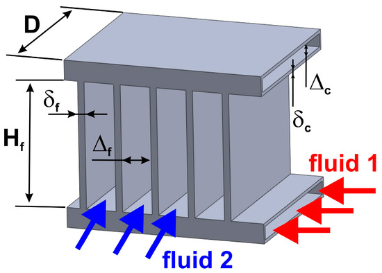
Figure 1.
Geometry and dimensions of the core of plate fin heat exchanger.
The core of an FFT (in other words, plate fin) heat exchanger can be almost fully characterized by the following dimensions: D—width, Hf—height of the fin, δf—thickness of the fin, Δf—gap between fins, δc—thickness of the wall of the plate channel, and Δc—internal thickness of the channel. As a whole unit that serves heat transfer from fluid 1 to fluid 2, the heat exchanger is characterized by the surface area of channels A (m2), area of fins Af (m2), thermal conductivity of metal λ, and heat transfer coefficients (HTCs) h1 and h2 (W/(m2 K)) between metal and fluid 1 and fluid 2, respectively.
The global coefficient of heat transfer UA (W/K) of the whole heat exchanger or, in other words, the reciprocal of thermal resistance between fluids 1 and 2, can be expressed as follows [25,26]:
where K = (A + Af)/A is the coefficient of surface extension and E is the effectiveness of the fins [23]. The latter value for rectangular fins placed between two channels can be expressed as follows [27,28]:
As the plate channels are flat and thin ducts, in a case when the flow of fluid 1 is fully developed and laminar, the Nusselt number of fluid 1 is close to constant Nu ≈ 8 [29]. Consequently, the heat transfer coefficient h1 for the metal–fluid 1 interface can be written as follows:
where λ1 is the thermal conductivity of fluid 1 and Φc is hydraulic diameter of the channel Φc = 4DΔc/(2D + 2Δc).
h1 = Nu/(λ1 Φc),
When the heat exchanger serves as Adsorber Heat Exchanger (ADHex) in AHT, and the granules of adsorbent are placed between fins, the coefficient of heat transfer h2 between the metal surface and granules can also be considered as constant [30]. Typical values of h2 lie in a range of h2 = 50 ÷ 200 W/(m2 K) [31]. However, when the heat exchanger serves as air-to-liquid radiator, and fluid 2 (air) flows around the plane fins, the air side Nusselt number and h2 can correlate with the velocity of air uair or, in other words, with the Reynolds number of air Reair. The classical formula for this correlation [32] is:
where Pr is the Prandtl number of fluid 2. However, if one considers non-ideal plates (perforated, zig-zag, wavy plates, etc.), instead of (4), the Nu-Re correlation can be rewritten in a more common form [33]:
where a, b, and c are empirical coefficients. For more complex cases (non-steady flow, presence of turbulence, etc.), a wide variety of correlations were proposed [34,35,36,37] that makes it possible to obtain values of Nu and h2 for any particular geometry of heat exchanging elements.
Nu = 0.664Re1/2Pr1/3,
Nu = aRebPrc,
Hence, knowing all the needed parameters of (1), one can easily calculate the global coefficient of heat transfer UA for a given heat exchanger. The results presented in [38] confirm this. In the cited work, a small heat exchanger with known geometry was fabricated with the use of a Yamaha Aerox YQ50 radiator as a core. For this purpose, this radiator was disassembled, an element of its core (125 mm × 43 mm × 26 mm) was extracted, and new aluminum side bars and fittings were welded to this piece. Then, this Hex was filled with an adsorbent and tested in a typical adsorption cycle of air conditioning (T evaporator = 10 °C, T condensation = 35 °C, T regeneration = 80 °C). The details of the adsorption experiments are presented in [38]. At the same time, UA and the maximal power that can be transferred from water to adsorbent for this Hex were theoretically calculated with the use of (1) and (2), and the results of the calculations were found to coincide reasonably with the experiment. In [30], nine ready-made automobile radiators were dismantled, and detailed information on the core geometry of these radiators was systematized. Then, three small heat exchanges with well-known geometry were fabricated and tested. Again, the results of experimental measurements of UA for these Hexes turned out to coincide well with calculated values of UA. This means that principally there are two different ways for finding the optimal heat exchanger among a large number of commercial radiators available on the market that fits the demands of a particular AHT application and ensures the desirable value of UA. The first way is to measure the UA directly under the real conditions of the AHT working cycle. The second way is to calculate UA, and this way looks easier than the first one. However, it requires detailed information on the radiator’s geometry (it means that the radiator must be opened) and knowledge on heat transfer coefficients. It should be noted that direct measurement of the HTC between adsorbent granules and plate metal support under realistic conditions of the AHT cycle needs significant value of efforts and time.
On the other hand, it should be remembered that, as mentioned above, FFT radiators were designed for applications that differ from adsorptive heat transformation. Originally, they serve as air-to-liquid heat exchangers, and, figuratively speaking, all the differences between the “role of the radiator” and the “role of ADHex” lie in the nature of the h2 coefficient. In the first case, the h2 coefficient characterizes convective heat transfer between air and metal; in the second case, h2 represents conductive heat transfer between solid grains and metal support. Evidently, the liquid side of the heat exchanger remains absolutely the same regardless of its role (radiator or ADHex). Therefore, a reasonable question arises: could it be that if a certain radiator shows high UA values among a number of different commercially available models, then the same will be true for the case of its usage as ADHex? Answering this question is the essence of this paper. In other words, the goal of this article is finding the link between thermal conductance of the air-to-liquid FFT radiator and its ability to ensure the maximal possible volumetric adsorption power in AHT. For this purpose, a set of small heat exchangers presented in [30,38] was tested in a wind tunnel, and values of UA (air-to-water) for them were measured in order to be compared with proper UA (adsorbent-to-water) values calculated with the use of Equations (1) and (2) and measured in [30,38]. This could open an alternative way, less labor-intensive but based on direct experimental measurement, for finding the optimal heat exchanger for AHT applications among the ready-made automobile radiators available in the market.
2. Materials and Methods
2.1. Small Heat Exchangers
Four small plate fin heat exchangers designated as R1–R4, presented and tested as ADHexes in [30,38], were used for investigations. Examples of the cores utilized for manufacturing the radiators are presented in Figure 2. It evidences that the geometry of each core visibly differs from the other, and Table 1, where the detailed information on the dimensions of the radiators is collected, confirms this fact. The assembled radiator consists of the core, which includes a certain number of plate channels and fins, side bars, and nozzles. All the parts are made of aluminum and are joined together with the use of the TIG welding technique.
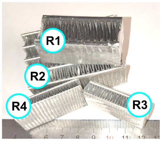
Figure 2.
Examples of cores used for manufacturing the radiators.

Table 1.
Geometry of the tested radiators.
Table 1 shows that volume of the cores for all radiators is almost the same and equals V = 140 ± 1 cm3, which allows correct comparison of UA values, because volumetric power (or in other words, volumetric conductance—UA related to unit volume) is one of the key characteristics of adsorbers and adsorptive heat transformers.
2.2. Wind Tunnel
The experimental test rig for the measurement of heat fluxes in air-to-water radiators consists of a wind tunnel, water circuit, and data acquisition system (Figure 3a). The wind tunnel is a rectangular thermally insulated duct where the tested radiator is placed. The tunnel serves as an air circuit and is equipped with a ventilator, flowmeter, and flow regulator. The water circuit serves for passing heat transfer liquid through the channels of the radiator and consists of a circulating thermocriostat, flowmeter, flow regulator, and pipelines. A set of 8 T-type thermocouples, an analog-to-digital converter, and a PC are the system for data collection. The thermocouples are positioned in a way allowing temperature measurement of inlet and outlet streams both in water and air circuits.
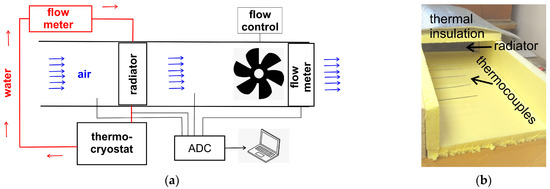
Figure 3.
(a) Scheme of the test rig; (b) View of the outlet part of wind tunnel.
In order to control temporal and spatial stability of air flow after the radiator, a set of five thermocouples was installed along the outlet part of the air duct. The joints of the T-couples were positioned on the duct’s axis with a pitch of 5 cm, as shown in Figure 3b.
2.3. Experimental Procedure and Data Evaluation
Before measurements, the tested radiator was placed inside the wind tunnel, connected to the water circuit, and then the test rig was properly thermally insulated in order to avoid heat losses. After that, certain values of water and air flows were set, and measurements were started. The temperature of inlet water was maintained stable at Tin(w) = 40 ± 0.1 °C, while the temperature of inlet air was not stabilized. During measurements, all the temperatures of inlet and outlet flows, both in air and water circuits, were recorded. Among five temperature readings that correspond to the outlet air flow, the maximal value of Tout(air) was taken. Typical temporal evolution of inlet and outlet temperatures in air and water circuits is presented in Figure 4. It evidences that within ~103 s after beginning the experiment, the temperatures and corresponding heat flows become stable.
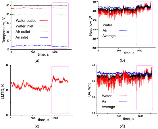
Figure 4.
Typical temporal evolution of: (a) Inlet and outlet temperature in water and air circuits; (b) Heat flow in water and air circuits and average value; (c) Logarithm Mean Temperature Difference; (d) Global heat transfer coefficient calculated for water and air circuits and average value. Radiator R3, air flow rate f(air) = 19.1 × 10⁻³ m3/s, water flow rate f(w) = 63.86 × 10⁻⁶ m3/s. Time interval when heat flows become stable is outlined in pink.
The rate of heat transfer in air Q(air) and water Q(w) circuits and average value Q(av) were defined as:
where Cp is heat capacity, ρ—density of air or water, respectively [39,40,41,42].
Q(air) = |(Tin(air) − Tout(air))∙ρ(air)∙Cp(air)∙f(air)|,
Q(w) = |(Tin(w) − Tout(w))∙ρ(w)∙Cp(w)∙f(w)|,
Q(av) = (Q(w) + Q(air))/2,
Logarithm mean temperature difference LMTD [28] represents the temperature driving force and is calculated as follows:
Finally, dividing the heat flow by the temperature driving force gives the global heat transfer coefficient UA:
UA(air) = Q(air)/LMTD,
UA(w) = Q(w)/LMTD,
UA(av) = Q(av)/LMTD,
An average value UA(av) was taken for further data treatment.
2.4. Error Analysis
The sources of instrumental errors are flowmeters (air flow meter—3%, water flow meter—2%), thermocouples, and ADC (±0.1 K), and all these errors contribute to uncertainties in the determination of heat flows, LMTD, and finally, UA. Assuming typical values of ΔT in the numerator of (9), for air circuit and for water circuit as ~15 K, ~20 K, and ~2 K, respectively, the absolute ε and relative ω errors for Q, LMTD, and UA can be estimated. The results of estimations are summarized in Table 2, and it evidences that the relative error in the determination of the average value of UA reaches 11.7%.
Table 2.
Sources of experimental errors and error analysis.
3. Results
3.1. Experimentally Measured UA
Figure 5 presents the dependences of global heat transfer coefficients UA measured for tested radiators on flows of air f(air) and water f(w). It evidences that UA for all radiators is weakly sensitive to water flow rate. This is in line with the statements of [29] on the constancy of the Nusselt number in thin flat channels with a laminar flow of HTF. On the contrary, in the case of the air flow, there is a noticeable sensitivity of the UA coefficient to the f(air) value. This indicates that, apparently, the coefficient of heat transfer h2 from air to metal depends on the velocity of the flow along the surface. Figure 5a indicates that radiator R1 is characterized by the lowest values of UA in a range UA = 5 ÷ 9 W/K. Radiator R2 in a range of air flow f(air) = 0.5 ÷ 1.5 × 10⁻² m3/s, which demonstrates UA almost twice higher than R1 (Figure 5b). In the same range of air flow, the UA coefficients for R3 and R4 radiators turned out to be close, especially in the interval f(air) = 0.5 ÷ 1.0 × 10⁻² m3/s (Figure 5b), while at higher flows radiator R4 shows significantly higher thermal conductance than R3 (UA = 65 W/K against 40 W/K).
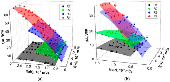
Figure 5.
Experimentally measured global heat transfer coefficients UA for radiators R1–R4 at various rates of air and water flow. Planes—polynomial fitting. (a) Whole range of air flow, (b) low air flows.
Generally, data presented evidence that the tested radiators are very different from each other, and with the same core volume, the UA values for them differ by more than five times. A common feature of radiators is a weak dependence of UA on the water flow in the channels and, conversely, a strong dependence on the air flow. Since the sections of both the water and air channels of the radiators are different, in order to correctly compare the dependences of UA on the flow, they should be converted into a dimensionless form.
3.2. Nusselt Number Correlations for Tested Radiators
The Reynolds numbers for water Re(w) and air Re(air) flows were calculated for the tested radiators as follows:
where u and ν are linear velocity and kinematic viscosity [41,42] of the corresponding fluid (water or air). The Nusselt number for the air–metal side Nu(air) can be written as follows:
Equations (1) and (2) give a one-to-one correspondence UA = function(h2) between the h2 coefficient and UA of the radiator with known geometry under the assumption that h1 = const (Equation (3)). Consequently, the dependence of the coefficient h2 on the UA will be described by the inverse function h2 = function−1(UA). It should be noted that because Equation (2) is a hyperbolic one, the inverse function is hardly to be written in analytical form. However, finding the coincidence between h2 and UA can be fulfilled for the entire experimental dataset using the graphical method, as is schematically demonstrated in Appendix A. Use of the experimental UA data algorithm for the finding of correlations between Nu and Re can be considered (Figure 6). First of all, UA = function(h2) should be plotted (h2 is the running parameter, e.g., from 0 to 300 W/(m2K)). After that, using the experimental value of UA, the heat transfer coefficient h2 can be found graphically (Appendix A). Nu and Re numbers can be calculated by Equations (14) and (15) using h2 and fair as parameters, respectively.
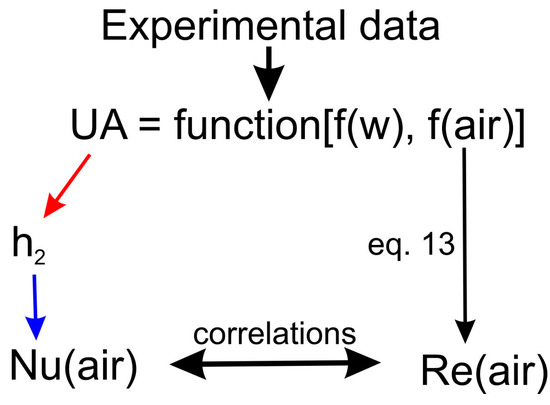
Figure 6.
Algorithm finding of correlations between Nu and Re using experimental data.
This makes it possible to find the appropriate correlations (Figure 7a, Figure 8a, Figure 9a, and Figure 10a). It turned out that for radiator R1, the correlation of Nu numbers with Re numbers is very close to a classical one (4). The correlations found for the R2 radiator (Table 3) somewhat differ from the classical one. For R3 and R4, it was found that Equations (4) and (5) are not suitable and function proposed by Hausen [33,37]; Nu ∝ (Rem − C), where m and C are constants, was used.
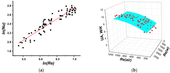
Figure 7.
(a) Nu number correlation for radiator R1; (b) Comparison of experimental data (red symbols) and approximation (blue 3D surface) calculated by found correlation.
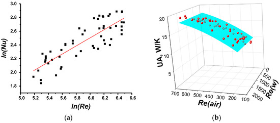
Figure 8.
(a) Nu number correlation for radiator R2; (b) Comparison of experimental data (red symbols) and approximation (blue 3D surface) calculated by found correlation.
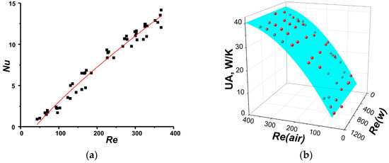
Figure 9.
(a) Nu number correlation for radiator R3; (b) Comparison of experimental data (red symbols) and approximation (blue 3D surface) calculated by found correlation.
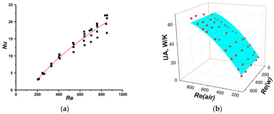
Figure 10.
(a) Nu number correlation for radiator R4; (b) Comparison of experimental data (red symbols) and approximation (blue 3D surface) calculated by found correlation.
Table 3.
Parameters for Nusselt number correlations of tested radiators.
The correlations found can be utilized for further scaling up the radiators, correct comparison of the radiator’s performance at various values of air flux, etc.
4. Discussion
The tested radiators were previously investigated [30] under conditions of adsorption air conditioning cycle (T evaporator = 10 °C, T condensation = 35 °C, T regeneration = 80 °C). Using Equations (1)–(3), data on the geometrical parameters of radiators (Table 1) assuming heat transfer coefficient h2 = 75 W/(m2K), as was done in [38] for a particular adsorbent–adsorbate working pair under real conditions of an adsorptive chilling cycle, one can easily calculate values of UA for all the considered radiators (Table 4).
Table 4.
Calculated by Equations (1)–(3) and experimentally measured [30] values of UA for tested radiators at working conditions of adsorptive air conditioning cycle.
These data presented in the second column of Table 4 coincide well with the results of direct experimental measurements (third column) performed in the adsorption test rig and reported in [30]. It is worth noting that the table shows the same tendency as Figure 5b, namely the lowest UA for R1 and the highest UA for R3, while radiator R2 occupies an intermediate position among them.
Therefore, the performed experiments and calculations showed that indeed, there is a visible coincidence between the performance demonstrated by the radiator in a wind tunnel and in adsorption heat transformation (Table 4). Thus, an alternative procedure of radiator selection can be proposed. In other words, instead of carrying out the adsorption experiment, one can easily check the radiator performance in the wind tunnel. Such an experiment is much simpler and faster and doesn’t require vacuum equipment. Moreover, for testing in a wind tube, a commercial radiator can be used as is, which would hardly be possible in an adsorption experiment.
Taking into account that tested radiators have different Hex’s surface of the core perpendicular to the direction of air flow (heights of core × length of core minus front surface of channels and fins), it is interesting to present experimental data in dimensionless coordinates (Figure 11a). Lines in Figure 11a show dependence of UA for considered radiators on Reair number. One can observe that in these coordinates, the tendency that was found earlier is also well pronounced: the highest UA for R3, the lowest UA for R1, with radiator R2 in the intermediate position. It is important that using this plot (Figure 11a), one can easily estimate the performance of any tested radiator if it will be filled with adsorbent with a known h2 value. For this purpose, the further algorithm should be used (Figure 11b): (1) using Equation (14) and known HTC h2, one can calculate the appropriate Nuair; (2) taking found correlations between Nu and Re numbers, the appropriate Re number can be found; (3) the UA which can be achieved using considered adsorbent and radiator can be found graphically. For example, for the adsorbent LiCl/SiO2 tested in [35], h2 = 75 W/(m2K) UA, demonstrated by R1–R4, is shown by open symbols (Figure 11a). One can see that h2 = 75 W/(m2K) for different radiators will be achieved at different and relatively low Re numbers (100–250). Therefore, for correct comparison of different radiators in the wind tube, it is important to find such Re numbers for each radiator which will correspond to the same needed value of h2 (metal-defined adsorbent).
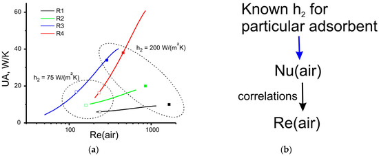
Figure 11.
(a) Global heat transfer coefficients UA for radiators vs. air Re number (lines) and appropriate UA calculated for different h2 values. Open symbols—h2 = 75 W/(m2K), solid symbols h2 = 200 W/(m2K); (b) Algorithm for estimation of UA for different sorbents.
Because the different adsorbents are characterized by different h2, it is interesting to discover possibilities of the proposed procedure for analysis of the performance of the aforementioned radiators if they will be filled with other sorption materials. For example, in [31], an adsorbent with h2 of approximately 200 W/(m2K) was tested. Figure 11a shows that for a sorbent with h2 = 75 W/(m2K), the UA values for radiators R3 and R4 are close, and in the case of a sorbent with h2 = 200 W/(m2K), the UA value for radiator R4 is higher. It is clear that in the case of a sorbent with h2 = 200 W/(m2K), radiators should be tested at higher Re numbers (Re > 300). Therefore, the proposed procedure, indeed, gives possibility for fruitful analyses of the performance of the adsorbent–Hex unit. Hence, the answer on the question posed in the introduction is definitely positive. Moreover, testing the radiators in a wind tunnel at various Re values potentially could give information as to whether the tested radiator is or is not optimal for usage with different adsorbents.
5. Conclusions
Four small representative Hexes made of commercial radiators with different core geometries were tested using a wind tunnel. Varying the flow of air (up to 3 × 10⁻² m3/s) and water (up to 7 × 10⁻⁵ m3/s), the values of the global heat transfer coefficient UA were measured. The UA values were found to correlate well with the data of sorption experiments described in the literature [30,38]. It was found that measured UA values are weakly dependent on water flow in contrast to air flow. The correlations between the Nusselt and Reynolds numbers were found and allow proposing an algorithm for choosing the proper commercial air-to-water radiators for use in adsorption heat transformers. It was demonstrated that the wind tunnel is effective for express assessment of using FFT radiators for adsorption heat conversion without destroying radiators or their direct testing in a complex adsorption installation requiring vacuum maintenance.
Author Contributions
Conceptualization, M.T. and A.G.; methodology, M.T.; validation, M.T. and A.G.; formal analysis, A.G.; investigation, I.K. and M.S.; resources, A.G.; data curation, I.K. and M.S.; writing—original draft preparation, A.G.; writing—review and editing, M.T.; visualization, A.G.; supervision, A.G.; project administration, A.G.; funding acquisition, A.G. All authors have read and agreed to the published version of the manuscript.
Funding
This research was funded by Russian Science Foundation, Grant Number 21-79-10183.
Data Availability Statement
Data are available on request from the corresponding author.
Acknowledgments
The authors are grateful to I.I. Gogonin for fruitful discussions.
Conflicts of Interest
The authors declare no conflict of interest.
Abbreviations
| ADC | analog to digital converter |
| ADHex | Adsorber Heat Exchanger |
| AHT | Adsorption Heat Transformation (Transformer) |
| FFT | finned flat tube |
| Hex | Heat Exchanger |
| HMT | heat mass transfer |
| Nomenclature | |
| a | coefficient |
| A | surface area, m2 |
| Cp | heat capacity, J/(g K) |
| D | width, m |
| E | effectiveness |
| f | flow rate, m3/s |
| H | height, m |
| h | heat transfer coefficient, W/(m2 K) |
| K | coefficient of surface extension |
| L | length, m |
| LMTD | logarithm mean temperature difference, K |
| Nu | Nusselt number |
| Pr | Prandtl number |
| Re | Reynolds number |
| Q | rate of heat transfer, W |
| T | temperature, K, °C |
| u | velocity, m/s |
| UA | global heat transfer coefficient, W/K |
| V | volume, cm3 |
| X | height of whole Hex, m |
| Subscripts | |
| 1, 2 | related to fluid 1 or 2 |
| air | related to air |
| c | channel |
| f | fin |
| in | inlet |
| out | outlet |
| Superscripts | |
| b, c | coefficients |
| Greek symbols | |
| δ | thickness, m |
| Δ | interval, m |
| λ | heat conductivity, W/(m K) |
| ε | absolute error, K |
| ω | relative error, % |
| Φ | hydraulic diameter, m |
| ρ | density, kg/m3 |
| ν | kinematic viscosity, m2/s |
Appendix A
Experimental UA data can be used for finding coincidence between UA and h2 values. First of all, UA = function(h2) should be plotted (h2 is the running parameter, e.g., from 0 to 300 W/(m2K)) (red lines in Figure A1, Figure A2, Figure A3 and Figure A4). After that, using the experimental value of UA (symbol), the heat transfer coefficient hf2 can be found graphically.

Figure A1.
Dependence of global heat transfer coefficient UA of radiator R1 on heat transfer coefficient h2 (red line) and element of experimental dataset (symbol). Arrows illustrate the principle of graphical solving of h2 = function−1 (UA).

Figure A2.
Dependence of global heat transfer coefficient UA of radiator R2 on heat transfer coefficient h2 (red line) and element of experimental dataset (symbol). Arrows illustrate the principle of graphical solving of h2 = function−1 (UA).

Figure A3.
Dependence of global heat transfer coefficient UA of radiator R3 on heat transfer coefficient h2 (red line) and element of experimental dataset (symbol). Arrows illustrate the principle of graphical solving of h2 = function−1 (UA).

Figure A4.
Dependence of global heat transfer coefficient UA of radiator R4 on heat transfer coefficient h2 (red line) and element of experimental dataset (symbol). Arrows illustrate the principle of graphical solving of h2 = function−1 (UA).
References
- Wang, R.; Wang, L.; Wu, J. Adsorption Refrigeration Technology: Theory and Application; John Wiley & Sons; Singapore Pte. Ltd.: Singapore, 2014. [Google Scholar]
- Meunier, F. Adsorption heat powered heat pumps. Appl. Therm. Eng. 2013, 61, 830–836. [Google Scholar] [CrossRef]
- Jakob, U.; Kohlenbach, P. Recent Developments of Sorption Chillers in Europe. IIR Bull. 2009, 34–40. [Google Scholar]
- Saghir, M.Z. Enhanced Energy Storage Using Pin-Fins in a Thermohydraulic System in the Presence of Phase Change Material. Fluids 2022, 7, 348. [Google Scholar] [CrossRef]
- Ezgi, C. Design and Thermodynamic Analysis of Waste Heat-Driven Zeolite–Water Continuous-Adsorption Refrigeration and Heat Pump System for Ships. Energies 2021, 14, 699. [Google Scholar] [CrossRef]
- Yonezawa, Y.; Matsushita, M.; Oku, K.; Nakano, H.; Okumura, S.; Yoshihara, M.; Sakai, A.; Morikawa, A. Adsorption Refrigeration System. U.S. Patent 4881376, 1989. [Google Scholar]
- Silica Gel Cooling Systems. Available online: https://fahrenheit.cool/en/chillers/adsorption-chillers/ (accessed on 5 December 2022).
- Mitsubishi, AQSOA Adsorption Heat Pump. Available online: http://www.aaasaveenergy.com/products/001/pdf/AQSOA_1210E.pdf (accessed on 5 December 2022).
- Saha, B.; Ng, K.S. (Eds.) Advances in Adsorption Technologies; Nova Science Publishers Inc.: Hauppauge, NY, USA, 2010. [Google Scholar]
- Hastürk, E.; Ernst, S.J.; Janiak, C. Recent advances in adsorption heat transformation focusing on the development of adsorbent materials. Current Opin. In Chem. Eng. 2019, 24, 26–36. [Google Scholar] [CrossRef]
- Miyazaki, T.; Akisawa, A.; Saha, B.B.; El-Sharkawy, I.I.; Chakraborty, A. A new cycle time allocation for enhancing the performance of two-bed adsorption chillers. Int. J. Refrig. 2009, 32, 846–853. [Google Scholar] [CrossRef]
- Choudhury, B.; Saha, B.B.; Chatterjee, P.K.; Sarkar, J.P. An overview of developments in adsorption refrigeration systems towards a sustainable way of cooling. Appl. Energy 2013, 103, 554–567. [Google Scholar] [CrossRef]
- Scherle, M.; Nowak, T.A.; Welzel, S.; Etzold, B.J.M.; Nieken, U. Experimental study of 3D–structured adsorbent composites with improved heat and mass transfer for adsorption heat pumps. Chem. Eng. J. 2022, 431, 133365. [Google Scholar] [CrossRef]
- Kowsari, M.; Niazmand, H.; Tokarev, M. Bed configuration effects on the finned flat-tube adsorption heat exchanger performance: Numerical modeling and experimental validation. Appl. Energy 2018, 213, 540–554. [Google Scholar] [CrossRef]
- Chang, W.; Wang, C.; Shieh, C. Experimental study of a solid adsorption cooling system using flat-tube heat exchangers as adsorption bed. Appl. Therm. Eng. 2007, 27, 2195–2199. [Google Scholar] [CrossRef]
- Grisel, R.J.H.; Smeding, S.F.; de Boer, R. Waste heat driven silica gel/water adsorption cooling in trigeneration. Appl. Therm. Eng. 2010, 30, 1039–1046. [Google Scholar] [CrossRef]
- Verde, M.; Cortés, L.; Corberán, J.M.; Sapienza, A.; Vasta, S.; Restuccia, G. Modelling of an adsorption system driven by engine waste heat for truck cabin A/C. Performance estimation for a standard driving cycle. Appl. Therm. Eng. 2010, 30, 1511–1522. [Google Scholar] [CrossRef]
- Verde, M.; Harby, K.; Corberan, J.M. Optimization of thermal design and geometrical parameters of a flat tube-fin adsorbent bed for automobile air-conditioning. Appl. Therm. Eng. 2017, 111, 489–502. [Google Scholar] [CrossRef]
- Togawa, J.; Kurokawa, A.; Nagano, K. Water sorption property and cooling performance using natural mesoporous siliceous shale impregnated with LiCl for adsorption heat pump. Appl. Therm. Eng. 2020, 173, 115241. [Google Scholar] [CrossRef]
- Zhu, L.Q.; Gong, Z.W.; Ou, B.X.; Wu, C.L. Performance Analysis of Four Types of Adsorbent Beds in a Double-Adsorber Adsorption Refrigerator. Proc. Eng. 2015, 121, 129–137. [Google Scholar] [CrossRef]
- Bendix, P.; Füldner, G.; Möllers, M.; Kummer, H.; Schnabel, L.; Henninger, S.; Henning, H.M. Optimization of power density and metal-to-adsorbent weight ratio in coated adsorbers for adsorptive heat transformation applications. Appl. Therm. Eng. 2017, 124, 83–90. [Google Scholar] [CrossRef]
- Rogala, Z. Adsorption chiller using flat-tube adsorbers–Performance assessment and optimization. Appl. Therm. Eng. 2017, 121, 431–442. [Google Scholar] [CrossRef]
- Papakokkinos, G.; Castro, J.; López, J.; Oliva, A. A generalized computational model for the simulation of adsorption packed bed reactors – Parametric study of five reactor geometries for cooling applications. Appl. Energy 2019, 235, 409–427. [Google Scholar] [CrossRef]
- Khatibi, M.; Kowsari, M.M.; Golparvar, B.; Hamid Niazmand, H.; Sharafian, A. A comparative study to critically assess the designing criteria for selecting an optimal adsorption heat exchanger in cooling applications. Appl. Therm. Eng. 2022, 215, 118960. [Google Scholar] [CrossRef]
- Handbook of Heat Transfer, 3rd ed.; Rohsenow, W.M., Hartnett, J.P., Cho, Y.I., Eds.; McGraw-Hill: London, UK, 1998. [Google Scholar]
- Duarte, J.A. Determination Global Heat Transfer Coefficient in Shell and Tube Type and Plates Heat Exchangers. In Proceedings of the International Refrigeration and Air Conditioning Conference, Paper 1260, Purdue, IN, USA, 16–19 July 2012. [Google Scholar]
- Huang, L.J.; Shah, R.K. Assessment of Calculation Methods for Efficiency of Straight Fins of Rectangular Profile. Int. J. Heat Fluid Flow 1992, 13, 282–293. [Google Scholar] [CrossRef]
- Ezgi, C. Basic Design Methods of Heat Exchanger. Heat Exchangers–Design, Experiment and Simulation; Murshed, S.S., Lopes, M.M., Eds.; IntechOpen: London, UK, 2017. [Google Scholar] [CrossRef]
- Erdoğan, M.E.; Imrak, C.E. The effects of duct shape on the Nusselt number. Math. Comp. Appl. 2005, 10, 79–88. [Google Scholar] [CrossRef]
- Grekova, A.D.; Tokarev, M.M.; Aristov, Y.I. Applying commercial heat exchangers for adsorption chillers: A finned flat-tube design. Appl. Therm. Eng. 2022; submitted. [Google Scholar]
- Graf, S.; Lanzerath, F.; Bardow, A. The IR-Large-Temperature-Jump method: Determining heat and mass transfer coefficients for adsorptive heat transformers. Appl. Therm. Eng. 2017, 126, 630–642. [Google Scholar] [CrossRef]
- Jiji, L.M. Heat Convection; Springer: Berlin/Heidelberg, Germany, 2009; p. 543. [Google Scholar] [CrossRef]
- Meyer, J.P.; Everts, M.; Coetzee, N.; Grote, K.; Steyn, M. Heat transfer coefficients of laminar, transitional, quasi-turbulent and turbulent flow in circular tubes. Int. Com. Heat Mass Transf. 2019, 105, 84–106. [Google Scholar] [CrossRef]
- Safaei, M.R.; Ahmadi, G.; Goodarzi, M.S.; Kamyar, A.; Kazi, S.N. Boundary Layer Flow and Heat Transfer of FMWCNT/Water Nanofluids over a Flat Plate. Fluids 2016, 1, 31. [Google Scholar] [CrossRef]
- Bertsche, D.; Knipper, P.; Meinicke, S.; Dubil, K.; Wetzel, T. Experimental Investigation on Heat Transfer Enhancement with Passive Inserts in Flat Tubes in due Consideration of an Efficiency Assessment. Fluids 2022, 7, 53. [Google Scholar] [CrossRef]
- Zandi, P.H.R.; Iovieno, M. Heat Transfer in a Non-Isothermal Collisionless Turbulent Particle-Laden Flow. Fluids 2022, 7, 7345. [Google Scholar] [CrossRef]
- Hausen, H. Heat Transfer in Counterflow, Parallel Flow and Cross Flow; McGrawHill: New York, NY, USA, 1983. [Google Scholar]
- Grekova, A.; Tokarev, M. An optimal plate fin heat exchanger for adsorption chilling: Theoretical consideration. Int. J. Thermofl. 2022, 16, 100221. [Google Scholar] [CrossRef]
- Thurnay, K. Thermal Properties of Water; Forschungszentrum Karlsruhe: Karlsruhe, Germany, 1995. [Google Scholar] [CrossRef]
- Harvey, A.H. Thermodynamic Properties of Water: Tabulation from the lAPWS Formulation 1995 for the Thermodynamic Properties of Ordinary Water Substance for General and Scientific Use; National Institute of Standards and Technology Boulder: Colorado, CO, USA, 1995; pp. 80303–83328. [Google Scholar]
- CoolPack: Refrigerant Calculations (Property Plots, Thermodynamic & Transport Properties, Comparison of Refrigerants). Available online: https://www.ipu.dk/products/coolpack/ (accessed on 6 December 2022).
- SecCool: A Program for Calculating, Comparing and Plotting Thermophysical Properties of Secondary Refrigerants. Available online: https://www.ipu.dk/products/seccool/ (accessed on 6 December 2022).
Disclaimer/Publisher’s Note: The statements, opinions and data contained in all publications are solely those of the individual author(s) and contributor(s) and not of MDPI and/or the editor(s). MDPI and/or the editor(s) disclaim responsibility for any injury to people or property resulting from any ideas, methods, instructions or products referred to in the content. |
© 2022 by the authors. Licensee MDPI, Basel, Switzerland. This article is an open access article distributed under the terms and conditions of the Creative Commons Attribution (CC BY) license (https://creativecommons.org/licenses/by/4.0/).