Scalable Simulation of Pressure Gradient-Driven Transport of Rarefied Gases in Complex Permeable Media Using Lattice Boltzmann Method

Abstract

Accurate representations of slip and transitional flow regimes present a challenge in the simulation of rarefied gas flow in confined systems with complex geometries. In these regimes, continuum-based formulations may not capture the physics correctly. This work considers a regularized multi-relaxation time lattice Boltzmann (LB) method with mixed Maxwellian diffusive and halfway bounce-back wall boundary treatments to capture flow at high Kn. The simulation results are validated against atomistic simulation results from the literature. We examine the convergence behavior of LB for confined systems as a function of inlet and outlet treatments, complexity of the geometry, and magnitude of pressure gradient and show that convergence is sensitive to all three. The inlet and outlet boundary treatments considered in this work include periodic, pressure, and a generalized periodic boundary condition. Compared to periodic and pressure treatments, simulations of complex domains using a generalized boundary treatment conserve mass but require more iterations to converge. Convergence behavior in complex domains improves at higher magnitudes of pressure gradient across the computational domain, and lowering the porosity deteriorates the convergence behavior for complex domains.

1. Introduction

Shale and tight systems comprise a wide range of physical scales in terms of flow and transport from nano- to micrometers [1]. The dominant physics of flow may vary widely among the various scales. As shown in Figure 1, flow regimes may be delineated using Knudsen number (Kn): (i) continuum flow regime (Kn < 0.001) where continuum fluid mechanics assumptions apply and flow may be described using the Navier–Stokes (N-S) equation with no-slip boundary conditions; (ii) slip flow regime (0.001 < Kn < 0.1) where N-S equation along with slip boundary conditions may be used; (iii) transitional flow regime (0.1 < Kn < 10) and free molecular flow regime (Kn > 10) [2,3]. In transitional and free molecular flow regime, flow behavior may not be described accurately via continuum-based assumptions [4]. Molecular dynamics (MD) simulations are effective in simulating transport and flow in confined systems at high Kn [5]. However, due to its computational cost, microscopic paradigms, such as MD simulation, are often not practical for relatively large domains [6]. In this work, we adopt the lattice Boltzmann (LB) method to simulate rarefied gas flow in complex geometries across a range of Kn. LB is a mesoscopic paradigm that incorporates the essential physics of microscopic processes and lends itself to parallel algorithms [7]. We account for slip and transitional regimes via mixed boundary treatments, and we use archival microscopic simulation data from the literature for validation. Such scalable implementations of physically accurate LB models across all relevant scales provide a framework for translating the physics between the pore and Darcy scales in hierarchical disordered media, such as shales and tight geologic media [8].

LB has been used with increasing frequency in the past few decades in part due to significant improvements in available computational power [9]. LB is used in various applications, such as heat transfer, aerodynamics, flow through permeable media and wave propagation [8,9,10,11], prediction of absolute, and relative permeability in conventional reservoir development, such as in sandstones [9,12,13,14], investigation of the effect of fluid and geometrical properties on wettability, capillary pressure, and relative permeability [15,16,17]. Wettability alteration phenomena in porous media is studied using LB extensively as a part of CO₂ sequestration and EOR processes [18,19,20]. LB is also successfully implemented in porous media characterization in terms of pore size distribution, tortuosity, and absolute permeability [21,22,23].

Technologies, such as scanning electron microscopy (SEM) [24] and scanning transmission electron microscopy (STEM) have enabled characterization of the fabric and pore structure of shales and tight formations in detail [25]. Nanoscale characterization techniques elucidate geometric details of the pore network structure of shales and tight formations. These pore networks may be used as the computational domain for LB to simulate flow under high Kn, which require careful design and implementation of boundary treatments to capture non-zero slip velocities [4].

The simplest wall boundary treatment is the bounce back (BB) approach, which requires that the particles colliding with the walls be reflected in the opposing direction. BB does not capture non-zero slip velocities, which are often encountered in high Kn scenarios [26]. To address this deficiency, BB may be combined with other wall treatments, such as specular reflection (SR) or Maxwellian diffusive reflection (MDR). In specular reflection, the velocity component of particles colliding with the wall is reversed [27]. The latter scatters particles back based on the Maxwellian distribution [28]. SR and MDR individually may overpredict slip velocities at the walls, which is alleviated by their combination with BB [4]. BB boundary treatment may be combined with either SR or MDR to capture the slip velocity at the walls in simulations of gas flow in complex microchannels. An example is a combination of BB and MDR that was used to simulate flow of methane in a three-dimensional pore network, which was developed using nanometer-scale STEM images of a shale sample [25]. These simulations enable examination of transport property of the characterized sample by computing the apparent gas permeability [29].

Boundary conditions (BC) at the inlet and outlet also play an important role in numerical simulations of flow in confined systems. A common approach is the use of the periodic boundary condition, which uses body forces to induce flow. Periodic BC may result in non-mass-conservative implementations for complex geometries [30]. Alternatively, bounce back of non-equilibrium distributions may be used to enforce pressure and velocity boundary conditions [31]. This approach may be applied to various boundary geometries. A generalized periodic boundary condition is another approach that was developed to overcome the shortcoming of periodic BC while leveraging its simplicity and computational efficiency [32,33,34].

This work presents a detailed analysis of different BCs for simple and complex nanoconfined systems. We elucidate the combined effects of pressure gradient and geometrical complexity on the computational efficiency and mass conservation of periodic, pressure, and generalized periodic inlet–outlet treatments. The remainder of this paper is organized in the following order: We describe the fundamentals of regularized MRT LB with a combination of diffusive and bounce back wall boundary treatments and three different inlet–outlet conditions. These include periodic, pressure [31], and generalized periodic boundary conditions. Next, we detail the implementation strategy and use microscale simulation data from the literature to validate the LB simulation results. Finally, we present sensitivity analyses of the three inlet–outlet conditions and wrap up the paper with a discussion and conclusions.

2. Lattice Boltzmann

2.1. Fundamentals

LB is a descendant of lattice gas automata, designed to mimic the behavior of fluid by means of density distribution functions. [35] derived the lattice Boltzmann equation in the following form:

$$f_{\alpha }\left(\mathit{x}+c{\mathit{e}}_{\alpha }\delta t, t+\delta t\right)-f_{\alpha }\left(\mathit{x}, t\right)={\Omega }_{\alpha }\left(f\left(\mathit{x}, t\right)\right)+\delta t{F}_{\alpha }\left(\mathit{x}, t\right),$$

(1)

where $f_{\alpha }\left(\mathit{x}, t\right)$ denotes the density distribution function in the discrete direction α at position $\mathit{x}$ and time $t$, ${\mathit{e}}_{\alpha }$ is a vector describing the direction of each discrete movement. Following this convention, we use the two-dimensional, nine-velocity model called D2Q9 as

$${\mathit{e}}_{\alpha }=\left\{\begin{array}{c}\left(0,0\right), \alpha =0\\ \left(1,0\right), \left(0, 1\right), \left(-1,0\right), \left(0,-1\right) \alpha =1, \dots , 4\\ \left(1, 1\right), \left(-1, 1\right), \left(-1,-1\right), \left(1,-1\right) \alpha =5, \dots , 8 \end{array}\right.$$

(2)

In LB, $c$ is the lattice speed, which is the ratio of lattice distance, $\delta x$, to lattice time step, $\delta t$, and it is set to one. ${\mathit{F}}_{\alpha }$ is the forcing term and is set to zero in our work. ${\Omega }_{\alpha }\left(f\left(\mathit{x}, t\right)\right)$ is the collision operator, which describes the rate of change in the distribution function during collision. An early collision operator is the BGK operator that was proposed by [36] as

$${\Omega }_{\alpha }\left(f\left(\mathit{x}, t\right)\right)=-\frac{1}{\tau }\left(f_{\alpha }-f_{\alpha }^{eq}\right),$$

(3)

where $\tau$ is the parameter representing the rate of relaxation toward equilibrium. This operator is called the single relaxation time (SRT), where the equation of kinematic viscosity is given by [37],

$$v=\frac{1}{6}\left(2\tau -1\right),$$

(4)

with $\tau >\frac{1}{2}$ as a condition. Despite the simplicity of SRT, BGK may lead to numerical instability at lower viscosities [38]. To overcome this shortcoming, a multiple-relaxation-time (MRT) collision scheme was proposed as [38,39],

$${\Omega }_{\alpha }\left(f\left(\mathit{x}, t\right)\right)=-{\displaystyle \sum }_{\beta }{\left({\mathit{M}}^{-1}\mathit{S}\mathit{M}\right)}_{\alpha ,\beta } \left(f_{\beta }-f_{\beta }^{eq}\right),$$

(5)

where $\mathit{M}$ transforms distribution functions onto the moment space. For the D2Q9 model, the calculation procedure for $\mathit{M}$ can be found in [38]. In the MRT scheme, each directional distribution function relaxes at a different rate, ${\tau }_{\alpha }$, represented by the diagonal matrix $\mathit{S}$ as

$$\mathit{S}=diag{\left({\tau }_{\rho }, {\tau }_e, {\tau }_{\epsilon },{\tau }_j,{\tau }_q,{\tau }_j,{\tau }_q,{\tau }_s,{\tau }_s \right)}^{-1},$$

(6)

where ${\tau }_{\rho }={\tau }_j=1$ represent the conserved quantities mass and momentum, ${\tau }_e$ and ${\tau }_{\epsilon }$ are given by [40] as ${\tau }_e=1.1$ and ${\tau }_{\epsilon }=1.2$. The shear viscosity term ${\tau }_s$ is proposed by [41] as

$${\tau }_s=\frac{1}{2}+\sqrt{\frac{2}{6}}\frac{NKn}{1+aKn},$$

(7)

where $a=2$, $N=\frac{H}{{\delta }_{\mathit{x}}}$ represent the local characteristic length, and $Kn$ is the local Kn defined as

$$Kn=\frac{\lambda }{L},$$

(8)

where $L$ is the dimensionless characteristic pore size, and $\lambda$ is mean free path, which is defined as

$$\lambda =\frac{kT}{4\pi \sqrt{2}{R}^{2}P},$$

(9)

where $k$ is Boltzmann constant, $T$ is the temperature, $R$ is molecular diameter, and $P$ is the pressure. ${\tau }_q$ is related to the slip velocity [24] by

$${\tau }_q=\frac{1}{2}+\frac{3+\pi {\left(2{\tau }_s-1\right)}^2{C}_2}{8\left(2{\tau }_s\right)-1},$$

(10)

where $C_2=0.9$.

The discrete equilibrium distribution function is given by a second order Taylor expansion of the Maxwell–Boltzmann distribution [42] as

$$f_{\alpha }^{eq}\left(\mathit{x}, t\right)=w_{\alpha }\rho \left(\mathit{x}, t\right)) \left(1+\frac{e_{\alpha }·u\left(\mathit{x}, t\right)}{{\left(c_s\right)}^2}+\frac{{(e_{\alpha }·u\left(\mathit{x}, t\right))}^2}{2{\left(c_s\right)}^4}-\frac{u\left(\mathit{x}, t\right)·u\left(\mathit{x}, t\right)}{2{\left(c_s\right)}^2}\right)$$

(11)

where the weighting factor $w_{\alpha }$ is defined as

$$w_{\alpha }=\left\{\begin{array}{c}\frac{4}{9}, \alpha =0\\ \frac{1}{9}, \alpha =1, ... 4\\ \frac{1}{36}, \alpha =5,...8.\end{array}\right.$$

(12)

$c_s=\frac{1}{\sqrt{3}}$ is the lattice speed of sound. The macroscopic density and velocity, $\rho$ and $\mathit{u}$, are calculated as

$$\rho \left(\mathit{x}, t\right)={\displaystyle \sum }_{\alpha }{f}_{\alpha }\left(\mathit{x}, t\right); \rho u\left(\mathit{x}, t\right)={\displaystyle \sum }_{\alpha }{\mathit{e}}_{\alpha }{f}_{\alpha }\left(\mathit{x}, t\right).$$

(13)

2.2. Regularization

The equilibrium distribution (Equation (11)) retains a second-order accuracy [43]. Due to the higher-order terms, the non-equilibrium part of the distribution may not be projected using a second order Hermite orthonormal basis denoted by ${ℍ}^2$. This may introduce error in the collision step [34]. To mitigate this issue, the regularization procedure proposed by [44,45] is used. The total distribution function is expressed as

$$f_{\alpha }=f_{\alpha }^{eq}+f_{\alpha }^{\prime },$$

(14)

where $f_{\alpha }^{\prime }$ is the non-equilibrium part of the distribution and is expressed in terms of Hermite polynomials as

$$\widetilde{f_{\alpha }}=w_{\alpha }\left(\frac{1}{{\left(2c_s\right)}^2} {\mathcal{H}}^2\left(\frac{{\mathit{e}}_{\alpha }}{c_s}\right){\displaystyle \sum }_{\beta }{f}_{\beta }^{\prime }{\mathit{e}}_{\beta }{\mathit{e}}_{\beta }\right),$$

(15)

where ${\mathcal{H}}^2$ is second order Hermite polynomial and is expressed as

$${\mathcal{H}}^2\left(e\right)={\mathit{e}}_{\beta }{\mathit{e}}_{\beta }-{\delta }_{\alpha \beta },$$

(16)

where ${\delta }_{\alpha \beta }$ is Kronecker delta. Replacing the non-regularized distribution, $f_{\alpha }^{\prime }$, with its regularized counterpart, $\widetilde{f_{\alpha }}$, in (Equation (14)) and combining it with (Equation (1)) produces the regularized MRT LBM collision equation operator:

$$f_{\alpha }\left(\mathit{x}+c{e}_{\alpha }\delta t, t+\delta t\right)=f_{\alpha }^{eq}+\widetilde{f_{\alpha }}-{\displaystyle \sum }_{\beta }{\left({\mathit{M}}^{-1}\mathit{S}\mathit{M}\right)}_{\alpha ,\beta }\widetilde{f_{\beta }}+\delta t{\mathit{F}}_{\alpha }\left(\mathit{x}, t\right).$$

(17)

2.3. Wall Boundary Treatment

The combination of bounce-back and Maxwellian diffusive boundary condition (BBDM) may be used to capture the slip velocity in slip and transitional flow regimes, as defined by

$$f_{\alpha }=r{f}_{\alpha }^{D\mathit{M}}+\left(1-r\right)f_{\alpha }^{BB},$$

(18)

where $f_{\alpha }^{D\mathit{M}}$ is the Maxwellian diffusion component at the wall, $f_{\alpha }^{BB}=f_{\sigma }$ and ${\mathit{e}}_{\alpha }=-e_{\sigma }$ is the bounce-back component, and $r$ is a constant that determines the contribution of each component. The Maxwellian diffusion component is calculated as

$$f_{\alpha }^{D\mathit{M}}=K,$$

(19)

where

$$K=\frac{{\sum }_{{\mathit{\xi }}_{\alpha }^{\prime }·\mathit{n}<0}\left|{\mathit{\xi }}_{\alpha }^{\prime }·\mathit{n}\right|f_{\alpha }}{{\sum }_{{\mathit{\xi }}_{\alpha }^{\prime }·\mathit{n}>0}\left|{\mathit{\xi }}_{\alpha }^{\prime }·\mathit{n}\right|f_{\alpha }^{eq} },$$

(20)

with ${\mathit{\xi }}_{\alpha }^{\prime }={\mathit{e}}_{\alpha }-{\mathit{u}}_w·\mathit{n}$, $\mathit{n}$ is the unit vector normal to the wall, and ${\mathit{u}}_w$ is the wall velocity. The parameter $r$ is defined as [46].

$$r=\frac{2C_1}{\sqrt{6/\pi }+C_1}.$$

(21)

This wall boundary condition satisfies the second-order slip velocity given by [4]

$${\mathit{u}}_s=C_{1}Kn\frac{\partial \mathit{u}}{\partial \mathit{n}}{|}_w-C_{2}K{n}^2\frac{{\partial }^2\mathit{u}}{\partial {\mathit{n}}^2}{|}_w,$$

(22)

where the coefficients $C_1=0.6$ and $C_2=0.9$ are used in (Equation (21)) and (Equation (10)).

2.4. Open Flow Boundary Conditions

In flow problems where matter may flow in and out of the domain, some of the distribution functions at the inlet and outlet may be undefined [30]. Suppose we have a computational domain as shown in Figure 2. At the inlet, $x=0$, the distribution functions entering the domain, (Equation (2)), are $f_1, f_5,$ and $f_8$. At the outlet, $x=Nx$, the distribution functions entering the domain are $f_3, f_6,$ and $f_8$. During propagation, these distribution functions will require special treatment. Three different inlet–outlet treatments for flow problems are discussed. The choice of open flow boundary conditions is based on the goal of analyzing the impact of the magnitude of the pressure gradient on convergence behavior. Other BCs are discussed in the literature [47] and are beyond the scope of this work.

2.5. Constant Pressure Inlet-Outlet Condition

The unknown distribution functions at the inlet and outlet may be found by fixing the density and calculating the velocities as [31],

$$\begin{gathered} u_{x,0}=1-\frac{f_0^0+f_2^0+f_4^0+2\left(f_3^0+f_6^0+f_7^0\right)}{{\rho }_0}, \\ {u}_{x,Nx}=\frac{f_0^{Nx}+f_2^{Nx}+f_4^{Nx}+2\left(f_1^{Nx}+f_5^{Nx}+f_8^{Nx}\right)}{{\rho }_{Nx}}-1. \end{gathered}$$

(23)

The velocities $u_{x,0}$ and $u_{x,Nx}$ are variable for $y=0, \dots , Ny$ while densities ${\rho }_0$ and ${\rho }_{Nx}$ are constant. The superscript of the distribution functions represents the $x$ coordinates. The following set of equations are derived using the bounce-back rule for distribution functions at the inlet and the outlet with the assumption that the tangential velocity, $u_y$, is zero at the inlet and outlet layers.

$$\begin{gathered} f_1^0=f_3^0+\frac{2}{3}{\rho }_0{u}_{x, 0}, \\ {f}_5^0=f_7^0-\frac{1}{2}\left(f_2^0-f_4^0\right)+\frac{1}{6}\left({\rho }_0{u}_{\mathit{x}, 0}\right), \\ {f}_8^0=f_6^0+\frac{1}{2}\left(f_2^0-f_4^0\right)+\frac{1}{6}\left({\rho }_0{u}_{x, 0}\right), \\ {f}_3^{Nx}=f_1^{Nx}-\frac{2}{3}{\rho }_{Nx}{u}_{x, Nx}, \\ {f}_6^{Nx}=f_8^{Nx}+\frac{1}{2}\left(f_4^{Nx}-f_2^{Nx}\right)-\frac{1}{6}\left({\rho }_{Nx}{u}_{x, Nx}\right), \\ {f}_7^{Nx}=f_5^{Nx}-\frac{1}{2}\left(f_4^{Nx}-f_2^{Nx}\right)-\frac{1}{6}\left({\rho }_{Nx}{u}_{x, Nx}\right). \end{gathered}$$

(24)

2.6. Periodic Boundary Conditions

Periodic BCs are computationally efficient and use external body forces to drive the flow in a repeating pattern. It is debatable how well body forces represent a given pressure gradient. However, as we will see later, the density profile does not appear to follow the pressure drop along the direction of flow. Moreover, the accuracy of periodic boundary in most of the cases is questionable due to the non-uniform cross sections in the complex geometries [48]. The general formulation of simple periodic boundary is implemented by [49].

$$\begin{gathered} f_{{\alpha }^{\prime }}^0=f_{{\alpha }^{\prime }}^{Nx}, \\ {f}_{{\beta }^{\prime }}^{Nx}=f_{{\beta }^{\prime }}^0. \end{gathered}$$

(25)

Here, ${\alpha }^{\prime }=1, 5, 8$ are the distributions leaving the domain at the outlet and are transferred to the inlet, and ${\beta }^{\prime }=3, 6, 7$ are distributions that leave the domain at the inlet and are transferred to the outlet layer.

2.7. Generalized Periodic Inlet–Outlet Condition

Varying pressure profiles along the domain cannot be represented by a simple periodic inlet–outlet condition. To explicitly set a pressure gradient while retaining periodicity, we use the generalized periodic inlet–outlet condition proposed by [33],

$${\rho }_0^y={\rho }_{Nx}^y+\left({\rho }_{in}-\overline{{\rho }_{Nx}^y}\right),$$

(26)

where ${\rho }_0^y$ and ${\rho }_{Nx}^y$ are density values at the inlet and outlet averaged along the $y$ axis, ${\rho }_{in}$ is the fixed density at the inlet ($x=0$), and $\overline{{\rho }_{Nx}^y}$ is the density at the outlet layer averaged along the $y$ axis. Averaging all, ${\rho }_0^y, y=0,\dots ,Ny$ will produce a fixed ${\rho }_{in}$ value. Correspondingly, the densities at the outlet are calculated as.

$${\rho }_{Nx}^y={\rho }_0^y+\left({\rho }_{out}-\overline{{\rho }_0^y}\right).$$

(27)

Once the density is calculated, the unknown distribution functions depicted in Figure 2 are

$$\begin{gathered} f_{i, 0}^y=f_i^{eq, y}\left({\rho }_{in},u{x}_{Nx}^y\right)+f_{i, Nx}^y, \\ {f}_{i, Nx}^y=f_i^{eq, y}\left({\rho }_{out},u{x}_0^y\right)+f_{i, 0}^y. \end{gathered}$$

(28)

In (Equation (28)), values $i=1, 5, 8$ correspond to the inlet and $i=3,6,7$ to the outlet.

3. Implementation Strategies

In order to achieve high performance and simulate a large number of domains, the following steps are taken: (i) The code is developed in C++ and is written to be cache friendly by using standard C++ vectors; (ii) variables are referenced inside subroutines to avoid the overhead associated with copying massive vectors. Linearized vectors require additional operations to map the lattice indices from 1D onto 2D and vice versa in non-local operations, such as streaming and bounce-back calculations. Typically, in LB codes, the variables that store the digital domain contain both pore and solid nodes. Therefore, an “if” statement is required to differentiate between pores and solids in local operations such as collision, equilibrium distribution calculation, and regularization. This method is called direct addressing (see Algorithm 1).

Algorithm 1. Computation of equilibrium distribution with direct addressing—vector “pore” stores domain information, vector “feq” stores equilibrium distribution, and “argin” is for additional variables, such as density and velocity distributions.
1	void computeEquilibrium(vector <double> &feq, vector <int> &pore, argin) {
2	for (int i = 0; i < pore.size(); i++)
3	if (pore[i] ==1)
4	feq[i] = getEquilibrium(argin);
5	}

For non-local operations, the situation becomes slightly more complex, because not only does the algorithm need to know if the current cell is void or not, but also the information regarding neighboring lattices must also be known. Therefore, an extra operation is needed to find the neighboring lattices along with an extra “if” statement to check if each neighbor is void or not (see Algorithm 2).

Algorithm 2. Pseudo-code for non-local operation with direct addressing—vector “f” stores distribution functions, “pore” stores domain information, and “argin” is for additional variables, such as local pore size and velocity vectors used in D2Q9; the subroutine “findNeighbor” is used for mapping of 1D indices onto 2D and finding the corresponding neighbors and mapping them back onto 1D.
1	void streamBB(vector <double> &f, vector <int> &pore, argin) {
2	for (int i = 0; i<pore.size(); i++)
3	if (pore[i] == 1)
4	for (int c = 0; c < 9; c++)
5	pore_neighbor_id = findNeighbor(i, c, argin);
6	if (pore[pore_neighbor_id] == 1)
7	stream(vector <double> &f, argin);
8	else
9	bounceBack(vector <double> &f, argin);}

Although the implementation of direct addressing is straightforward, it is not computationally efficient. The alternative approach is indirect addressing where indices of pore nodes and their neighbors are stored prior to the start of simulation (see Algorithm 3). This helps to avoid “if” statements and mapping of indices in every timestep and decreases the number of iterations.

Algorithm 3. Finding pore indices before the start of simulation—“ids_pores” stores all the indices of pore nodes, “stream_from_ids” stores current indices where particles are streaming from, “stream_to_ids” stores the corresponding neighbors, and “bounceback_ids” stores lattices where bounce back is to be executed.
1	Vector <int> ids_pores;
2	for (int i = 0; i < pore.size(); i++)
3	if (pore[i] == 1)
4	ids_pores.push_back(i);
5	vector <int > stream_from_ids;
6	vector <int> stream_to_ids;
7	vector <int> bounceback_ids;
8	for (int i = 0; i < pore.size(); i ++)
9	if (pore[i] == 1)
10	for (int c = 0; c < 9; c++)
11	pore_neighbor_id = findNeighbor(i, c);
12	if (pore[pore_neighbor_id] == 1)
13	stream_from_ids.push_back(i);
14	stream_to_ids.push_back(pore_neighbor_id);
15	else
16	bounceback_ids.push_back(i);

Algorithm 3 represents the preprocessing stage for the core operations of LB and is only executed once in each simulation to store all the necessary indices that are static. With these indices in hand, local (see Algorithm 4) and non-local operations are executed more efficiently. The time it takes to extract indices is negligible compared to the overall runtime.

Algorithm 4. Local operation with direct addressing.
1	void computeEquilibrium(vector <double> &feq, vector <int> &ids_pores, *argin) {
2	for (int i = 0; i< ids_pores.size(); i++)
3	feq[ids_pores[i]] = getEquilibrium(*argin);
4	}

Notice that in Algorithm 5 streaming and bounce back steps are independent loops. This means that they can be executed in parallel. For example, a 1000 × 1000 domain with 10% porosity includes a total of 1,000,000 lattices, 100,000 of which are void. The collision step in direct addressing would iterate 1 million times as opposed to 100,000 iterations required by indirect addressing. Figure 3 demonstrates the runtime comparison of direct and indirect addressing with different porosities. The simulation domain on which we carried out the runtime test is shown in Figure A2 where different porosities are achieved by varying individual channel diameters. It is worth noting that the runtime differences do not shrink at higher porosities as opposed to typical implementation of indirect addressing [50].

Algorithm 5. Non-local operation with indirect addressing.
1	void streamBB(vector <double> &f, vector <int> & stream_from_ids, vector <int> & stream_to_ids, vector <int> & boundary_ids, argin) {
2	for (int i = 0; i < stream_from_ids.size(); i++)
3	stream(f, stream_from_ids[i], stream_to_ids[i], argin);
4	for (int i = 0; i < boundary_ids.size(); i++)
5	bounceback(f, boundary_ids[i], argin); }

Next, we implement hybrid parallelization to further increase the performance. We use OpenMP for multithreading and MPI for multiprocessing. In multithreading, all the threads are bound to one process and can have shared memory. Multiprocessing is, however, slightly more complicated due to non-local operations: each process has its own memory, and information can only be shared through communication subroutines.

As shown in Figure 4, the computational domain is divided into subdomains for processes. Each process loads its own portion of the data and performs initialization. Then, each process launches a predefined number of threads for hybrid parallelization. Local operations are performed without the need for communications and processes do not have to wait for each other. The streaming step is divided into two parts. In part 1, each process executes streaming and boundary operations in lattices where communications are not required (striped areas in Figure 4). In part 2, non-local operations in lattices that are shown as blank in Figure 4 are performed. In the second part, processes need to communicate with each other. First, each process stores pore node indices and distribution functions in its blank section in vectors. Then, neighboring processes exchange corresponding data vectors and perform non-local (stream and bounce-back) calculations within the blank sections. There are two advantages to separating non-local operations into two parts. Firstly, it does not require an overlap between subdomains, thus avoiding extra memory use. Secondly, all communications are carried out simultaneously. Communication subroutines are the bottleneck of multiprocessing. Therefore, as much information as possible should be exchanged between processes to increase performance while overlapped with local computing tasks. The first and last processes communicate with each other to calculate inlet and outlet distribution functions when periodic and generalized periodic conditions are used. This step is not implemented for the pressure BC since no such information is required to perform inlet–outlet distribution calculations. Figure 5 compares the runtime with a different number of cores and processes for the simulation domain shown in Figure A2.

4. Validation

The model is validated in a variety of domains. The simplest domain consists of slit nano-channels with Kn ranging from 0.01 to 10. LB is run with all three inlet–outlet treatments, and the results are compared against direct simulation Monte Carlo (DSMC) data from the literature [43]. As shown in Figure 6, the results of LB with all three inlet–outlet BCs agree with DSMC data.

The model is also validated in a domain with a square obstacle as shown in Figure 7. Figure 8 shows a comparison between streamwise velocity results from LB with periodic, pressure, and generalized periodic BCs at Kn = 0.11 against MD data [43]. Overall, in all cases, generalized periodic BC produces results that are closer to reference data.

The domain shown in Figure 9 is adapted from [43]. The domain comprises a simple channel with a triangular obstacle with a stair-wise boundary. We simulate flow in this domain using LB with three different inlet–outlet boundary conditions at $Kn=0.15$. The results are compared with archival MD simulation data from the literature [43] in Figure 10. The differences between periodic, pressure, and generalized periodic boundary conditions are more pronounced near the inlet and outlet compared to the middle of the domain. The generalized periodic BC produces more accurate results compared to the other two considered boundary condition types.

Next, we compare the pressure drop across a simple slit nanopore comparing all three inlet–outlet BCs. Inspired by [32], we devise a 21 × 21 simulation domain similar to Figure 2 with a lattice resolution of 0.15 nm, an outlet pressure of 2.0 MPa, and a pressure gradient of 10 kPa/m with no obstacle in the channel. As shown in Figure 11, the body forces used to induce flow in the periodic BC do not appear to generate a drop in pressure (density) between two ends of the domain. The regions near the inlet and the outlet exhibit nonlinear pressure gradients produced by the pressure inlet–outlet BC [31] in a simple nano-channel. Finally, the generalized periodic BC produces a smooth linear gradient bounded by the fixed inlet and outlet pressures and densities.

Finally, we perform a mesh refinement study using the periodic boundary condition in a slit pore with a diameter of 50 nm. Mesh size is varied from 20 × 20 to 40 × 40 while keeping the physical conditions the same. As shown in Figure 12, the differences in normalized streamwise velocity are more pronounced at the boundaries. The differences between 35 × 35 and 40 × 40 are nearly negligible. Motivated by these results, we use a mesh resolution of 1 nm to minimize the impact of mesh size at the boundaries.

5. Results and Discussion

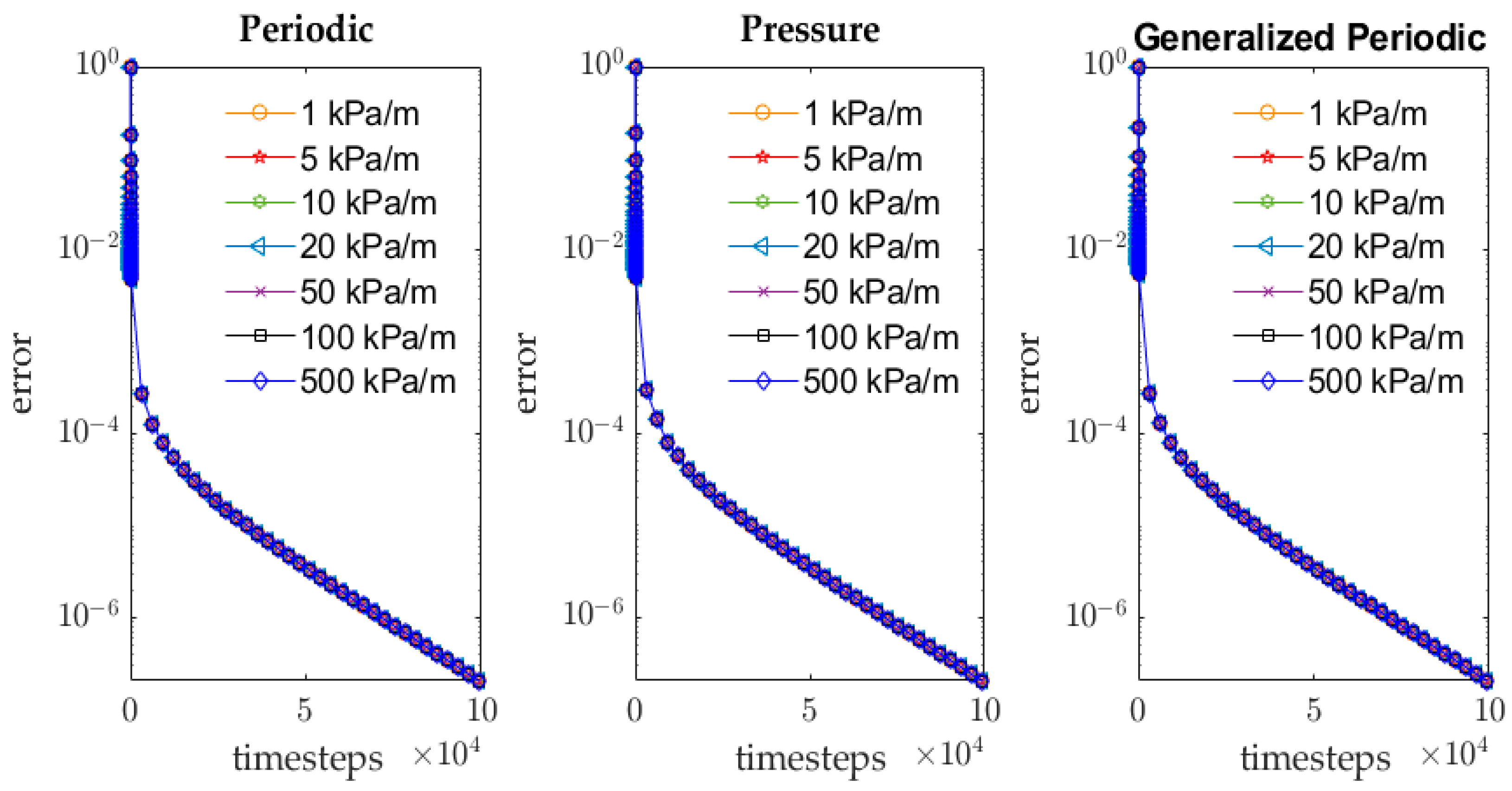
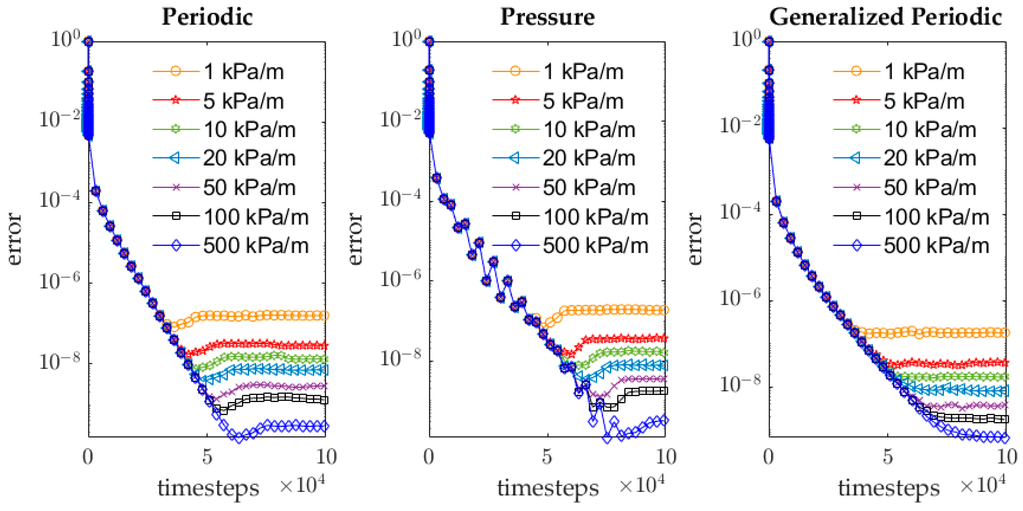
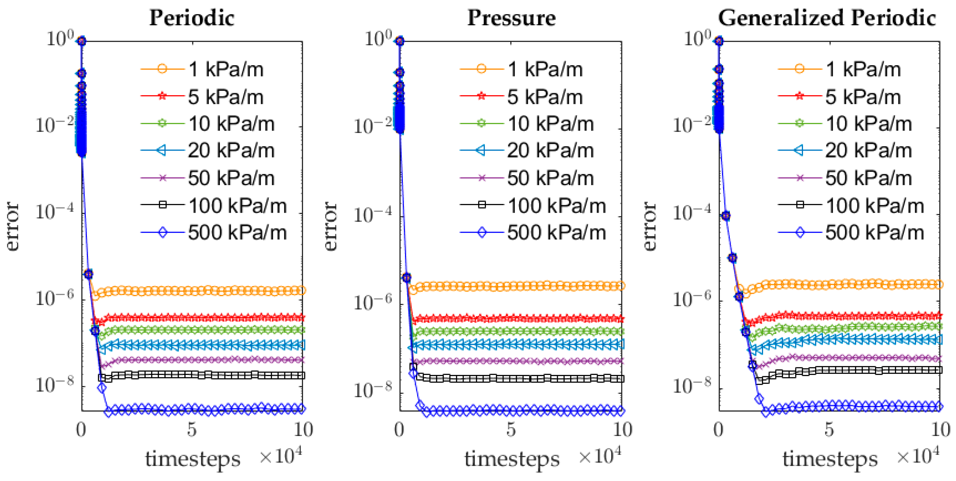
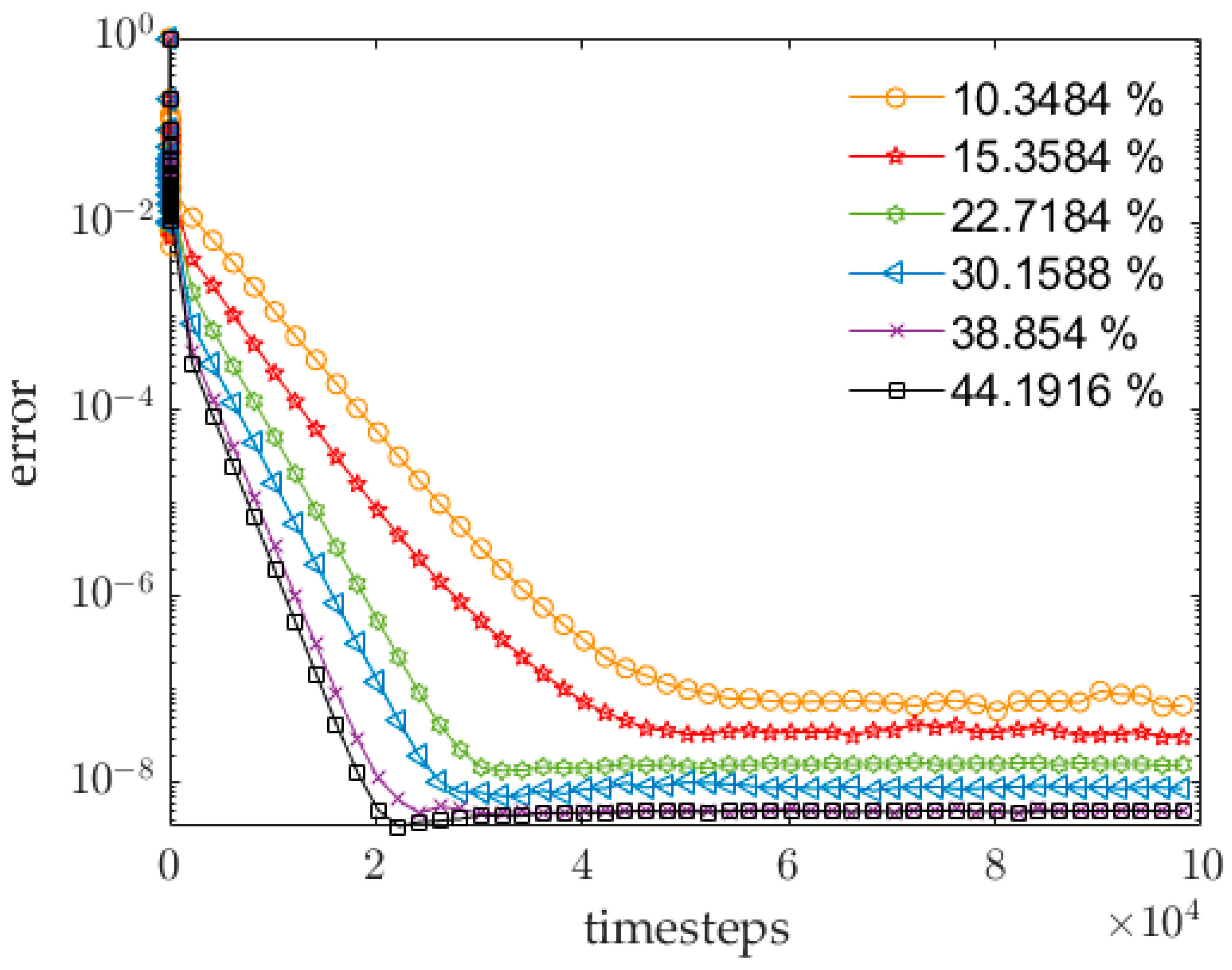
5.1. Convergence Behavior Sensitivity to Pressure Gradient and Complexity

We analyze the convergence behavior of LB with different inlet–outlet BCs under different pressure gradients to assess the speed of convergence [51]. We conduct 63 different simulations on 3 different domains: Domain D1 uses a 500 × 500 mesh in a simple channel with no obstacles (Figure 2), domain D2 uses a 500 × 500 mesh in a channel with a triangular obstacle in the middle (Figure A1), and domain D3 uses a 500 × 500 mesh in a complex network of channels (Figure A2).

$$E=\frac{{\sum }_{i=1}^N(u_i^{t-1}-u_i^t)}{{\sum }_{i=1}^N{u}_i^t},$$

(29)

The simulations are carried out under 7 different pressure gradients ranging from 1 kPa/m to 500 kPa/m. All simulations are run for 100 k timesteps, and the error is calculated using Equation (29) where $i$ represents cells and $t$ represents timestep.

Figure 13 summarizes results of 21 simulations on a simple computational domain. The simulations of the specified pressure gradients behave the same and almost converge at the same final error of approximately 2.0 × 10⁻⁷. This behavior is reasonable given the domain size and simplicity. There is a total of a quarter million cells in the domain 99% of which are void space. As a result, the convergence behavior does not change significantly due to changes in the pressure gradient. Furthermore, in large simple domains, the inlet and outlet layers’ contribution to the overall simulation behavior is rather small, meaning that the inlet–outlet boundary condition does not affect the convergence—see Figure 13. Mass flow rates, however, change significantly—see

Table A1. Mass Flow rate results.

		D1			D2			D3
	Gradient (kPa/m)	Inlet Mass (kg/s)	Outlet Mass (kg/s)	Absolute Difference	Inlet Mass (kg/s)	Outlet Mass (kg/s)	Absolute Difference	Inlet Mass (kg/s)	Outlet Mass (kg/s)	Absolute Difference
Periodic	1	8.18 × ${10}^{-5}$	8.18 × ${10}^{-5}$	0.0	1.57 × ${10}^{-5}$	1.57 × ${10}^{-5}$	3.44 × ${10}^{-12}$	3.77 × ${10}^{-7}$	3.77 × ${10}^{-7}$	6.19 × ${10}^{-11}$
	5	4.09 × ${10}^{-4}$	4.09 × ${10}^{-4}$	0.0	7.84 × ${10}^{-5}$	7.84 × ${10}^{-5}$	4.84 × ${10}^{-12}$	1.88 × ${10}^{-6}$	1.88 × ${10}^{-6}$	3.06 × ${10}^{-10}$
	10	8.18 × ${10}^{-4}$	8.18 × ${10}^{-4}$	0.0	1.57 × ${10}^{-4}$	1.57 × ${10}^{-4}$	6.88 × ${10}^{-12}$	3.77 × ${10}^{-6}$	3.77 × ${10}^{-6}$	6.11 × ${10}^{-10}$
	20	1.64 × ${10}^{-3}$	1.64 × ${10}^{-3}$	0.0	3.13 × ${10}^{-4}$	3.13 × ${10}^{-4}$	1.14 × ${10}^{-11}$	7.54 × ${10}^{-6}$	7.54 × ${10}^{-6}$	1.22 × ${10}^{-9}$
	50	4.09 × ${10}^{-3}$	4.09 × ${10}^{-3}$.	0.0	7.84 × ${10}^{-4}$	7.84 × ${10}^{-4}$	1.97 × ${10}^{-11}$	1.88 × ${10}^{-5}$	1.88 × ${10}^{-5}$	3.05 × ${10}^{-9}$
	100	8.18 × ${10}^{-3}$	8.18 × ${10}^{-3}$	0.0	1.57 × ${10}^{-3}$	1.57 × ${10}^{-3}$	4.77 × ${10}^{-11}$	3.77 × ${10}^{-5}$	3.77 × ${10}^{-5}$	6.10 × ${10}^{-9}$
	500	4.09 × ${10}^{-2}$	4.09 × ${10}^{-2}$	0.0	7.84 × ${10}^{-3}$	7.84 × ${10}^{-3}$	2.45 × ${10}^{-10}$	1.88 × ${10}^{-4}$	1.88 × ${10}^{-4}$	3.05 × ${10}^{-8}$
Pressure	1	6.79 × ${10}^{-5}$	6.79 × ${10}^{-5}$	6.37 × ${10}^{-10}$	1.30 × ${10}^{-5}$	1.30 × ${10}^{-5}$	7.23 × ${10}^{-10}$	3.06 × ${10}^{-7}$	3.06 × ${10}^{-7}$	4.10 × ${10}^{-11}$
	5	3.40 × ${10}^{-4}$	3.40 × ${10}^{-4}$	7.88 × ${10}^{-10}$	6.51 × ${10}^{-5}$	6.51 × ${10}^{-5}$	6.06 × ${10}^{-10}$	1.53 × ${10}^{-6}$	1.53 × ${10}^{-6}$	1.33 × ${10}^{-9}$
	10	6.79 × ${10}^{-4}$	6.79 × ${10}^{-4}$	7.32 × ${10}^{-10}$	1.30 × ${10}^{-4}$	1.30 × ${10}^{-4}$	6.86 × ${10}^{-10}$	3.06 × ${10}^{-6}$	3.06 × ${10}^{-6}$	3.04 × ${10}^{-9}$
	20	1.36 × ${10}^{-3}$	1.36 × ${10}^{-3}$	7.28 × ${10}^{-10}$	2.60 × ${10}^{-4}$	2.60 × ${10}^{-4}$	7.66 × ${10}^{-10}$	6.12 × ${10}^{-6}$	6.13 × ${10}^{-6}$	6.47 × ${10}^{-9}$
	50	3.40 × ${10}^{-3}$	3.40 × ${10}^{-3}$	8.27 × ${10}^{-10}$	6.51 × ${10}^{-4}$	6.51 × ${10}^{-4}$	7.09 × ${10}^{-10}$	1.53 × ${10}^{-5}$	1.53 × ${10}^{-5}$	1.68 × ${10}^{-8}$
	100	6.79 × ${10}^{-3}$	6.79 × ${10}^{-3}$	5.75 × ${10}^{-10}$	1.30 × ${10}^{-3}$	1.30 × ${10}^{-3}$	6.40 × ${10}^{-10}$	3.06 × ${10}^{-5}$	3.06 × ${10}^{-5}$	3.39 × ${10}^{-8}$
	500	3.40 × ${10}^{-2}$	3.40 × ${10}^{-2}$	1.60 × ${10}^{-9}$	6.51 × ${10}^{-3}$	6.51 × ${10}^{-3}$	2.86 × ${10}^{-10}$	1.53 × ${10}^{-4}$	1.53 × ${10}^{-4}$	1.71 × ${10}^{-7}$
Generalized Periodic	1	6.81 × ${10}^{-5}$	6.81 × ${10}^{-5}$	0.0	1.30 ×${10}^{-5}$	1.30 × ${10}^{-5}$	0.0	3.13 × ${10}^{-7}$	3.13 × ${10}^{-7}$	0.0
	5	3.41 × ${10}^{-4}$	3.41 × ${10}^{-4}$	0.0	6.51 × ${10}^{-5}$	6.51 × ${10}^{-5}$	0.0	1.57 × ${10}^{-6}$	1.57 × ${10}^{-6}$	0.0
	10	6.81 × ${10}^{-4}$	6.81 × ${10}^{-4}$	0.0	1.30 × ${10}^{-4}$	1.30 × ${10}^{-4}$	0.0	3.13 × ${10}^{-6}$	3.13 × ${10}^{-6}$	0.0
	20	1.36 × ${10}^{-3}$	1.36 × ${10}^{-3}$	0.0	2.61 × ${10}^{-4}$	2.61 × ${10}^{-4}$	0.0	6.27 × ${10}^{-6}$	6.27 × ${10}^{-6}$	0.0
	50	3.41 × ${10}^{-3}$	3.41 × ${10}^{-3}$	0.0	6.51 × ${10}^{-4}$	6.51 × ${10}^{-4}$	1.08 × ${10}^{-18}$	1.57 × ${10}^{-5}$	1.57 × ${10}^{-5}$	0.0
	100	6.81 × ${10}^{-3}$	6.81 × ${10}^{-3}$	1.04 × ${10}^{-17}$	1.30 × ${10}^{-3}$	1.30 × ${10}^{-3}$	0.0	3.13 × ${10}^{-5}$	3.13 × ${10}^{-5}$	0.0
	500	3.41 × ${10}^{-2}$	3.41 × ${10}^{-2}$	0.0	6.51 × ${10}^{-3}$	6.51 × ${10}^{-3}$	0.0	1.57 × ${10}^{-4}$	1.57 × ${10}^{-4}$	0.0

.

The simulations using domain D2 (with a triangular obstacle) exhibit different behavior compared to the results from domain D1. Data in Figure 14 indicate that lower pressure gradients result in a faster convergence but at higher errors. The error in each simulation starts to fluctuate around a certain value and does not diminish any further after a certain number of timesteps. These fluctuations are more pronounced when a pressure boundary condition is applied.

The convergence behavior in the complex domain D3 (Figure 15) is quite different from those in D2 and seem to converge considerably faster.

Table 1. Summary of final error values.

	D1	D2	D3
Periodic	1.99 × ${10}^{-7}$	2.86 × ${10}^{-10}$	2.99 × ${10}^{-9}$
Pressure	1.96 × ${10}^{-7}$	3.19 × ${10}^{-10}$	3.97 × ${10}^{-9}$
Generalized Periodic	1.96 × ${10}^{-7}$	6.73 × ${10}^{-10}$	3.74 × ${10}^{-9}$

shows the error values at the end of each simulation with the pressure gradient set to 500 kPa/m. Simulations with a periodic boundary condition often converge at the smaller errors.

Additional simulations are carried out using domain D3 to further explore the effect of complexity on convergence behavior. Different versions of the complex computational domain (Figure A2) with different porosities are generated by varying individual channel diameters. Simulations are run in these domains at a pressure gradient of 500 kPa/m using the generalized periodic BC. As shown in Figure 16, the convergence behavior appears to improve as the porosity of the domain increases while other parameters are kept constant.

5.2. Mass Conservation

The data presented thus far explore the convergence behavior of LB under different conditions and open boundary conditions. To validate mass conservation, the inlet and outlet mass rates at the end of each simulation are shown in Table A1. These results are from the three computational domains (D1, D2, and D3), at different pressure gradients, and using different boundary conditions. In D1, periodic and generalized periodic BCs conserve mass. With the introduction of an obstacle (D2), the periodic BC fails to conserve mass. In all cases, the generalized periodic BC appears to conserve mass while the pressure BC fails to do so. It is worth noting that the absolute difference between inlet and outlet mass rates in the cases of periodic and pressure BCs become more pronounced as the complexity increases.

6. Problem Significance and Future Work

Simulation of the transport of rarefied gases at high Kn presents challenges related to accuracy and convergence of the results. This work investigates the behavior of different inlet–outlet BCs as the impact of the driving forces. As shown in Figure 8 and Figure 10, unlike simple periodic BC, pressure and generalized BCs are well-suited for flow and transport in nanopores with complex geometries. The main concern related to these BCs is the computational expense. In choosing the BC, one must consider the relative complexity of the algorithm, computational expense, and the convergence behavior, Figure 3, Figure 5 and Figure 16.

The geometries considered in the computational domains in this work capture the typical geometries and pore morphologies that are often encountered in both classical subsurface reservoirs [24,52] and tight formations [25]. The presented framework enables simulation of transport of gases at high Kn in complex pore networks that are often encountered in geologic media. A careful selection of implementation strategies aids in decreasing the computational expense significantly. Additionally, an analysis of the convergence behavior as a function of the magnitude of the driving force may inform a practicable convergence tolerance. The simulation of the domain in Figure A2 showcases the potential impact of the convergence tolerance on the computational expense for complex systems while retaining accuracy using a generalized periodic BC. By contrast, periodic BC is preferable in simple geometries, such as slit nanopores, due to its simplicity and superior convergence behavior. Future extensions of this work may comprise simulation of larger and more complex systems and inclusion of intermolecular forces to study adsorption behavior in nanoconfined systems.

7. Conclusions

This work considers different boundary conditions, namely periodic, pressure, and generalized periodic BCs, in the context of a regularized MRT-LB that uses mixed Maxwellian diffusive and bounce-back boundary treatments to capture non-zero slip velocities for high Kn flows. The focus here is to examine combined effects of pressure gradient and domain complexity on convergence behavior and mass conservation. The results suggest that a higher-pressure gradient in all cases, except in simple channels, results in an improved convergence behavior of LB. The periodic BC results in the fastest convergence while the generalized periodic BC converges the slowest. Unlike the periodic BC, the generalized periodic BC may represent the pressure gradient reasonably well in slit nano-channels. The pressure BC may lead to unphysical behavior in the pressure gradients at the inlet and the outlet, which result in less accurate streamwise velocity profiles. In complex domains, the generalized periodic BC is superior to periodic and pressure BCs from a mass conservation standpoint. As a result, the generalized periodic BC appears to be the optimal choice for simulating domains with complex geometries where flow is driven by a pressure gradient.

References

1. Deng, H.; Hu, X.; Li, H.A.; Luo, B.; Wang, W. Improved pore-structure characterization in shale formations with FESEM technique. J. Nat. Gas Sci. Eng. 2016, 35, 309–319. [Google Scholar] [CrossRef]
2. Li, X.; Fan, J.; Yu, H.; Zhu, Y.; Wu, H. Lattice Boltzmann method simulations about shale gas flow in contracting nano-channels. Int. J. Heat Mass Transf. 2018, 122, 1210–1221. [Google Scholar] [CrossRef]
3. Chambre, P.A.; Schaaf, S.A. Flow of Rarefied Gases; Princeton University Press: Princeton, NJ, USA, 2017. [Google Scholar]
4. Wang, Y.; Aryana, S.A. Pore-scale simulation of gas flow in microscopic permeable media with complex geometries. J. Nat. Gas Sci. Eng. 2020, 81, 103441. [Google Scholar] [CrossRef]
5. Wu, H.; Chen, J.; Liu, H. Molecular Dynamics Simulations about Adsorption and Displacement of Methane in Carbon Nanochannels. J. Phys. Chem. C 2015, 119, 13652–13657. [Google Scholar] [CrossRef]
6. Yu, H.; Zhu, Y.; Jin, X.; Liu, H.; Wu, H. Multiscale simulations of shale gas transport in micro/nano-porous shale matrix considering pore structure influence. J. Nat. Gas Sci. Eng. 2019, 64, 28–40. [Google Scholar] [CrossRef]
7. Hanasoge, S.M.; Succi, S.; Orszag, S.A. Lattice Boltzmann method for electromagnetic wave propagation. EPL Europhys. Lett. 2011, 96, 14002. [Google Scholar] [CrossRef] [Green Version]
8. Mehmani, Y.; Anderson, T.; Wang, Y.; Aryana, S.A.; Battiato, I.; Tchelepi, H.A.; Kovscek, A.R. Striving to translate shale physics across ten orders of magnitude: What have we learned? Earth-Sci. Rev. 2021, 223, 103848. [Google Scholar] [CrossRef]
9. Liu, H.; Kang, Q.; Leonardi, C.R.; Schmieschek, S.; Narváez, A.; Jones, B.D.; Williams, J.R.; Valocchi, A.J.; Harting, J. Multiphase lattice Boltzmann simulations for porous media applications: A review. Comput. Geosci. 2016, 20, 777–805. [Google Scholar] [CrossRef] [Green Version]
10. Guo, S.; Feng, Y.; Jacob, J.; Renard, F.; Sagaut, P. An efficient lattice Boltzmann method for compressible aerodynamics on D3Q19 lattice. J. Comput. Phys. 2020, 418, 109570. [Google Scholar] [CrossRef]
11. Mishra, S.C.; Roy, H.K. Solving transient conduction and radiation heat transfer problems using the lattice Boltzmann method and the finite volume method. J. Comput. Phys. 2007, 223, 89–107. [Google Scholar] [CrossRef]
12. Ramstad, T. Simulation of Two-Phase Flow in Reservoir Rocks Using a Lattice Boltzmann Method. SPE J. 2010, 15, 917–927. [Google Scholar] [CrossRef]
13. Ramstad, T.; Idowu, N.; Nardi, C.; Øren, P.E. Relative Permeability Calculations from Two-Phase Flow Simulations Directly on Digital Images of Porous Rocks. Transp. Porous Media 2012, 94, 487–504. [Google Scholar] [CrossRef]
14. Xu, M.; Liu, H. Prediction of immiscible two-phase flow properties in a two-dimensional Berea Sandstone using the pore-scale lattice Boltzmann simulation. Eur. Phys. J. E 2018, 41, 124. [Google Scholar] [CrossRef] [PubMed]
15. Guiltinan, E.J.; Santos, J.E.; Cardenas, M.B.; Espinoza, D.N.; Kang, Q. Two-phase fluid flow properties of rough fractures with heterogeneous wettability: Analysis with lattice Boltzmann simulations. Water Resour. Res. 2020, 56, e2020WR027943. [Google Scholar] [CrossRef]
16. Ghasemi, S.; Moradi, B.; Rasaei, M.R.; Rahmati, N. Near miscible relative permeability curves in layered porous media- investigations via diffuse interface lattice Boltzmann method. J. Pet. Sci. Eng. 2022, 209, 109744. [Google Scholar] [CrossRef]
17. Li, Z.; Galindo-Torres, S.; Yan, G.; Scheuermann, A.; Li, L. A lattice Boltzmann investigation of steady-state fluid distribution, capillary pressure and relative permeability of a porous medium: Effects of fluid and geometrical properties. Adv. Water Resour. 2018, 116, 153–166. [Google Scholar] [CrossRef]
18. Nemer, M.N.; Rao, P.R.; Schaefer, L. Wettability alteration implications on pore-scale multiphase flow in porous media using the lattice Boltzmann method. Adv. Water Resour. 2020, 146, 103790. [Google Scholar] [CrossRef]
19. An, S.; Zhan, Y.; Mahani, H.; Niasar, V. Kinetics of wettability alteration and droplet detachment from a solid surface by low-salinity: A lattice-boltzmann method. Fuel 2022, 329, 125294. [Google Scholar] [CrossRef]
20. Akai, T.; Blunt, M.J.; Bijeljic, B. Pore-scale numerical simulation of low salinity water flooding using the lattice Boltzmann method. J. Colloid Interface Sci. 2020, 566, 444–453. [Google Scholar] [CrossRef]
21. Viberti, D.; Peter, C.; Salina Borello, E.; Panini, F. Pore structure characterization through path-finding and lattice Boltzmann simulation. Adv. Water Resour. 2020, 141, 103609. [Google Scholar] [CrossRef]
22. Zhao, J.; Qin, F.; Derome, D.; Kang, Q.; Carmeliet, J. Improved pore network models to simulate single-phase flow in porous media by coupling with lattice Boltzmann method. Adv. Water Resour. 2020, 145, 103738. [Google Scholar] [CrossRef]
23. Cheng, Z.; Ning, Z.; Wang, Q.; Zeng, Y.; Qi, R.; Huang, L.; Zhang, W. The effect of pore structure on non-Darcy flow in porous media using the lattice Boltzmann method. J. Pet. Sci. Eng. 2018, 172, 391–400. [Google Scholar] [CrossRef] [Green Version]
24. Guo, F.; Aryana, S.A.; Wang, Y.; McLaughlin, J.F.; Coddington, K. Enhancement of storage capacity of CO2 in mega porous saline aquifers using nanoparticle-stabilized CO2 foam. Int. J. Greenh. Gas Control 2019, 87, 134–141. [Google Scholar] [CrossRef]
25. Frouté, L.; Wang, Y.; McKinzie, J.; Aryana, S.; Kovscek, A. Transport Simulations on Scanning Transmission Electron Microscope Images of Nanoporous Shale. Energies 2020, 13, 6665. [Google Scholar] [CrossRef]
26. Nie, X.; Doolen, G.D.; Chen, S. Lattice-Boltzmann Simulations of Fluid Flows in MEMS. J. Stat. Phys. 2002, 107, 279–289. [Google Scholar] [CrossRef]
27. Lim, C.Y.; Shu, C.; Niu, X.D.; Chew, Y.T. Application of lattice Boltzmann method to simulate microchannel flows. Fluids 2002, 14, 2299–2308. [Google Scholar] [CrossRef]
28. Ansumali, S.V.; Karlin, I. Kinetic boundary conditions in the lattice Boltzmann method. Phys. Rev. E 2002, 66, 026311. [Google Scholar] [CrossRef] [Green Version]
29. Ziarani, A.S.; Aguilera, R. Knudsen’s Permeability Correction for Tight Porous Media. Transp. Porous Media 2011, 91, 239–260. [Google Scholar] [CrossRef]
30. Krüger, T.; Kusumaatmaja, H.; Kuzmin, A.; Shardt, O.; Silva, G.; Viggen, E.M. The Lattice Boltzmann Method: Principles and Practice; Springer International Publishing: Cham, Switzerland, 2017. [Google Scholar] [CrossRef]
31. Zou, Q.; He, X. On pressure and velocity boundary conditions for the lattice Boltzmann BGK model. Phys. Fluids 1997, 9, 1591–1598. [Google Scholar] [CrossRef]
32. Gräser, O.; Grimm, A. Adaptive generalized periodic boundary conditions for lattice Boltzmann simulations of pressure-driven flows through confined repetitive geometries. Phys. Rev. E 2010, 82, 016702. [Google Scholar] [CrossRef]
33. Kim, S.H.; Pitsch, H. A generalized periodic boundary condition for lattice Boltzmann method simulation of a pressure driven flow in a periodic geometry. Phys. Fluids 2007, 19, 108101. [Google Scholar] [CrossRef]
34. Zhang, R.; Shan, X.; Chen, H. Efficient kinetic method for fluid simulation beyond the Navier-Stokes equation. Phys. Rev. E 2006, 74, 046703. [Google Scholar] [CrossRef] [Green Version]
35. He, X.; Luo, L.S. Theory of the lattice Boltzmann method: From the Boltzmann equation to the lattice Boltzmann equation. Phys. Rev. E 1997, 56, 6811–6817. [Google Scholar] [CrossRef] [Green Version]
36. Bhatnagar, P.L.; Gross, E.P.; Krook, M. A Model for Collision Processes in Gases. I. Small Amplitude Processes in Charged and Neutral One-Component Systems. Phys. Rev. 1954, 94, 511–525. [Google Scholar] [CrossRef]
37. Qian, Y.H.; D’Humières, D.; Lallemand, P. Lattice BGK Models for Navier-Stokes Equation. EPL Europhys. Lett. 1992, 17, 479–484. [Google Scholar] [CrossRef]
38. Lallemand, P.; Luo, L.S. Theory of the lattice Boltzmann method: Dispersion, dissipation, isotropy, Galilean invariance, and stability. Phys. Rev. E 2000, 61, 6546–6562. [Google Scholar] [CrossRef] [PubMed] [Green Version]
39. D’Humières, D.; Ginzburg, I.; Krafczyk, M.; Lallemand, P.; Luo, L.-S. Multiple–relaxation–time lattice Boltzmann models in three dimensions. Philos. Trans. R Soc. Lond Ser. Math. Phys. Eng. Sci. 2002, 360, 437–451. [Google Scholar] [CrossRef]
40. Guo, Z.; Zheng, C.; Shi, B. Lattice Boltzmann equation with multiple effective relaxation times for gaseous microscale flow. Phys. Rev. E 2008, 77, 036707. [Google Scholar] [CrossRef]
41. Li, Q.; He, Y.L.; Tang, G.H.; Tao, W.Q. Lattice Boltzmann modeling of microchannel flows in the transition flow regime. Nanofluidics 2011, 10, 607–618. [Google Scholar] [CrossRef]
42. Chen, H.; Chen, S.; Matthaeus, W.H. Recovery of the Navier-Stokes equations using a lattice-gas Boltzmann method. Phys. Rev. A 1992, 45, R5339–R5342. [Google Scholar] [CrossRef]
43. Suga, K. Lattice Boltzmann methods for complex micro-flows: Applicability and limitations for practical applications. Fluid Dyn. Res. 2013, 45, 034501. [Google Scholar] [CrossRef]
44. Latt, J.; Chopard, B. Lattice Boltzmann method with regularized pre-collision distribution functions. Math. Comput. Simul. 2006, 72, 165–168. [Google Scholar] [CrossRef]
45. Shan, X.; Yuan, X.F.; Chen, H. Kinetic theory representation of hydrodynamics: A way beyond the Navier–Stokes equation. J. Fluid Mech. 2006, 550, 413–441. [Google Scholar] [CrossRef]
46. Chai, Z. Gas Flow Through Square Arrays of Circular Cylinders with Klinkenberg Effect: A Lattice Boltzmann Study. Commun. Comput. Phys. 2010, 8, 1052–1073. [Google Scholar] [CrossRef]
47. Mohamad, A.A. Lattice Boltzmann Method: Fundamentals and Engineering Applications with Computer Codes, 2nd ed.; Springer: London, UK, 2019. [Google Scholar]
48. Zhang, J.; Kwok, D.Y. Pressure boundary condition of the lattice Boltzmann method for fully developed periodic flows. Phys. Rev. E 2006, 73, 047702. [Google Scholar] [CrossRef] [PubMed]
49. Maier, R.S.; Bernard, R.S.; Grunau, D.W. Boundary conditions for the lattice Boltzmann method. Phys. Fluids 1996, 8, 1788–1801. [Google Scholar] [CrossRef]
50. Narváez, A.; Harting, J. Evaluation of pressure boundary conditions for permeability calculations using the lattice-Boltzmann method. arXiv 2010, arXiv:1005.2322. [Google Scholar]
51. Rostamzadeh, A.; Razavi, S.E.; Mirsajedi, S.M. Towards multidimensional artificially characteristic-based scheme for incompressible thermo-fluid problems. Mechanics 2018, 23, 826–834. [Google Scholar] [CrossRef] [Green Version]
52. Guo, F.; Aryana, S.A. An Experimental Investigation of Flow Regimes in Imbibition and Drainage Using a Microfluidic Platform. Energies 2019, 12, 1390. [Google Scholar] [CrossRef]
Figure 1. Kn (see Equations (8) and (9)) as a function of pore size and pressure.
Fluids 08 00001 g001
Figure 2. Open flow boundary.
Fluids 08 00001 g002
Figure 3. Runtime of single LB iteration with direct and indirect addressing under different porosities.
Fluids 08 00001 g003
Figure 4. Visualization of multiprocessing.
Fluids 08 00001 g004
Figure 5. Single iteration of LB runtime: (a) multithreaded and (b) multiprocessor.
Fluids 08 00001 g005
Figure 6. Velocity profiles using three inlet–outlet treatments at different Kn. Y axes represent normalized streamwise velocity, and X axes represent the position across the channel.
Fluids 08 00001 g006
Figure 7. Simulation domain adapted from [43].
Fluids 08 00001 g007
Figure 8. Velocity profiles using three inlet–outlet treatments at different cross sections. Y axes represent normalized streamwise velocity, and X axes represents the position across the channel.
Fluids 08 00001 g008
Figure 9. Benchmark domain adapted from [42].
Fluids 08 00001 g009
Figure 10. Velocity profiles by LB with three inlet–outlet treatments at different cross sections. Y axis represents normalized streamwise velocity, and X axis represents the position across the channel.
Fluids 08 00001 g010
Figure 11. Pressure-drop results from generalized periodic, pressure, and periodic boundary conditions in a slit nanopore. Y axis represents pressure difference with respect to the outlet.
Fluids 08 00001 g011
Figure 12. Normalized streamwise velocity at different mesh sizes.
Fluids 08 00001 g012
Figure 13. Convergence behavior in domain D1.
Fluids 08 00001 g013
Figure 14. Convergence behavior in domain D2.
Fluids 08 00001 g014
Figure 15. Convergence behavior in domain D3.
Fluids 08 00001 g015
Figure 16. Convergence behavior at different porosity values shown in the legend.
Fluids 08 00001 g016