1. Introduction
Engine oil lubricates various rotating and sliding parts and functions as a buffer effect in areas subjected to high loads. A high-performance lubrication system is required to ensure safe and smooth operation of the engine in high-temperature, high-pressure, and high-speed operating environments. The overall demand for smaller and lighter engines has resulted in more stringent design requirements for the various components of the lubrication system. The engine oil is interposed between the piston and cylinder liner to provide a sealing effect, and it also provides a wide range of cooling effects. The role of the lubrication system is to deliver that oil to each part, collect it, adjust it to an appropriate state, and send it out. The engines of race cars and sports cars require a layout that saves space, reduces weight, and lowers the height from the floor to lower the center of gravity of the vehicle. For these reasons, an external tank is placed outside the engine according to the available space in the layout. Furthermore, the oil stored in this external tank is called a dry sump system, which allows for better separation of oil and air to prevent foaming. In race cars and sports cars, large acceleration and deceleration forces of 1 to 2 G are applied every few seconds. These forces can cause sloshing of the oil in the oil tank, degrading the oil–air separation performance and preventing normal lubrication and cooling of the engine. This dry sump system can reduce the size of the lower part from the crankshaft without the necessity of storing oil in the oil pan. There is less agitation of the oil by the crankshaft, and both the agitation resistance and the increase in oil temperature are smaller. However, in addition to the normal pump that pumps the oil, a scavenge pump is required to suck the oil that collects in the oil pan into the oil tank, and the scavenge pump has the disadvantage of easily sucking in air and blow-by gas at the same time as the oil. Some research has been performed on designs that prevent the pump from sucking air [
1]. The scavenge pump is often designed to have a flow rate more than twice that of the feed pump. In addition, about 8% to 10% of air is melted in the oil under atmospheric pressure, and the melted air becomes bubbles when the flow path is narrow and the pressure rapidly drops [
2]. Air bubbles in the oil cause a decrease in cooling performance, accelerated oil deterioration and sludge generation, and oil film breakage. They also have a serious impact on engine safety by increasing piping resistance, degrading the performance of oil-based radiators, and affecting the lubrication condition of opposing surfaces.
In the dry sump system, the defoaming capability of the oil side is limited because the oil is strongly agitated, and it is necessary to increase the separation capability by using a mechanism that separates the oil from the gas. A gas–liquid separation mechanism that separates bubbles from the oil by the difference in specific gravity using a swirling flow is useful for efficiently removing gas from the oil [
3,
4]. The parameters for separating air and oil using a swirl flow have been investigated by numerical calculations [
5]. However, the flow field is more complicated and includes anisotropic three-dimensional rotating flow, and there are many local secondary flows and other flow phenomena such as central recurrent flow, local circulating flow, and local short-circuit flow. At the same time, due to the presence of the two-phase mixture of oil and gas, the flow field also shows complex changes in the two-phase interface. All these factors add to the difficulty of the separator design and optimization process. In this dry sump system, oil circulating in the engine is collected in the oil tank by a scavenge pump to separate the oil from air and bubbles, and then pumped into the engine by the main oil pump as lubricating oil. The scavenge pump is often set to a discharge volume that requires to completely return the engine oil containing many bubbles discharged from the engine that is rotating or exploding to the oil tank. In other words, a mixture of about 50% air and 50% oil is put into the oil tank under normal use. The mixture must be separated quickly in the oil tank. Since the oil contains both easily separable air and small bubbles that are difficult to separate, it is extremely difficult to separate both quickly in a small volume. In particular, small bubbles in the oil must be carefully removed because they degrade the lubrication performance of the engine.
In a typical oil tank, the oil is spatially rotated along the inner wall of the tank by discharging it at a certain angle to the top of the tank. The centrifugal force generated by the spiral rotation pushes the oil with high specific gravity against the inner wall, and the air bubbles with low specific gravity gather on the central axis of the tank, resulting in gas–liquid separation. There is a strong demand for miniaturization of oil tanks, and each manufacturer has its own ideas. However, the design of oil tanks is based on the diameter experiment rule and experimental methods, and a method for selecting the shape parameters of each part of the mechanism considering various conditions has not been established. In previous studies, devices that remove air bubbles by means of swirling flow have not been investigated considering the front-to-back and side-to-side accelerations that occur during loading. Since the device uses the simple principle of separating and removing bubbles from a liquid by generating a swirling flow with the energy of the fluid, it can be used not only for engine oil but also for various other liquids.
Many separators have been studied to collect oil from the air and return it to the sump to meet emission regulations. The pressure drop and filter collection efficiency of 12 different crankcase oil mist separators were measured. In addition to filters, separators and cyclone separators were also investigated. The cyclone type was found to have a low pressure drop, although its supplemental efficiency was not high [
6]. A gas–liquid cyclone characterized by the generation of a swirling flow with guide vanes and uniform flow is proposed. The internal flow field and separation performance of this cyclone were investigated by numerical simulation. The larger the torsional angle, the higher the separation efficiency, but the larger the pressure drop [
7]. An analysis of the development of a liquid film in an upwelling (swirling) flow due to the action of centrifugal and gravitational fields in a cyclone chamber of a distribution system was discussed. The dynamics of the liquid film flow was analyzed with the help of three-dimensional and unsteady numerical simulations, and it was found that the flow fluctuations become smaller when the thickness of the liquid film is small, and the flow becomes homogeneous at the outlet of the device [
8]. In gas turbine engine transmission systems, shaft-bearing lubrication and cooling is typically provided by oil injected into bearing chambers sealed by pneumatic labyrinth seals. To improve the design of the separator, a computational model of the existing design was created and a two-phase coupled CFD calculation was performed. A limited amount of experimental data collected by particle image velocimetry (PIV) was used for validation [
9]. A new gas–liquid cyclone featuring the generation of swirling flow with guide vanes and uniform flow was designed. The internal flow field and separation performance of this cyclone were investigated by numerical simulation.
The purpose of this study is to improve the gas–liquid separation performance of the oil tank and to establish a design method to enable gas–liquid separation only in the oil tank. Since it is difficult for conventional oil tanks to completely remove bubbles remaining in the hydraulic oil, it is essential to introduce a technology to actively separate and remove bubbles from the oil. Therefore, the bubble removal performance was improved even under the condition of added lateral acceleration by appropriately generating a swirl flow. First, an acrylic model of an oil tank was used to verify the accuracy by performing CAE analysis using various turbulence models. Then, the parameters of the bubble remover, such as the size of the oil tank, were studied. In addition, the bubble removal performance under the condition of added lateral acceleration was examined.
2. Validation of CAE Analysis Accuracy
2.1. Experimental Apparatus
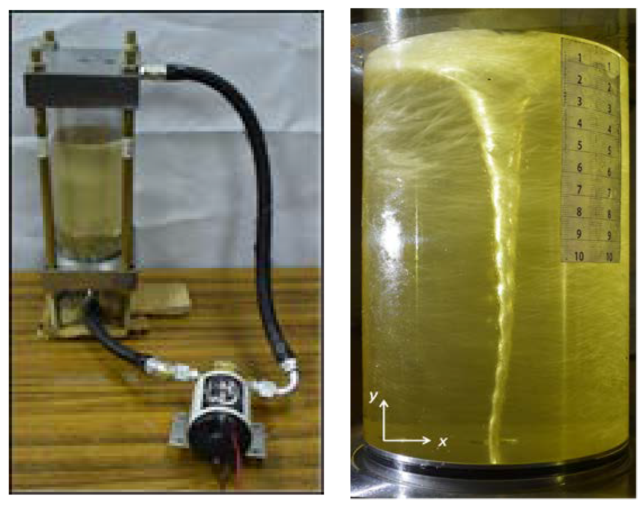
To verify the accuracy of the results of the CAE analysis, a visualization experiment of the flow inside the oil tank was conducted using an experimental apparatus made of transparent acrylic pipes. The experimental apparatus for visualization and an example of the flow in the oil tank taken from the experiment are shown in
Figure 1. The oil tank has a cylindrical shape, and the oil flows in from the top, generating a swirling flow along the circumference so that no bubbles are generated when the oil flows in. A gear pump is used to flow the oil into and out of the oil tank. The discharge section is located at the bottom center. The inflow rate was set to 1.7 × 10
−4 m
3/s, which is the maximum rate in the operating range of the actual machine. Oil with a kinematic viscosity of 1.08 Pa s was used. The oil tank was 100 mm in diameter and 250 mm in height, and the oil level was set at 200 mm from the bottom of the oil tank when the machine was stopped. It can be confirmed that a vortex was generated on the central axis of the tank and extended to the outflow pipe.
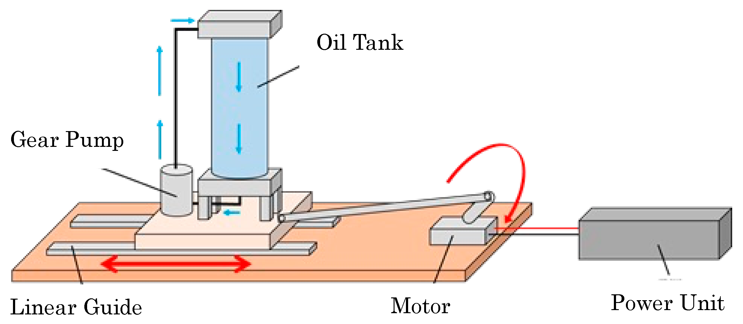
Next, an experimental apparatus was made to verify the accuracy of the analysis when periodic acceleration was applied. A schematic diagram of the experimental apparatus is shown in
Figure 2. A motor was rotated by a power supply, and periodic acceleration was added by a crank-slide mechanism. In the experiment, the periodic acceleration was 0.40 m/s
2 at 1 Hz.
The physical properties of the oils used in the experiments and CAE analysis were kinematic viscosity of 20 mm2/s and density of 8.7 × 10² kg/m3, respectively. The kinematic viscosity of WAKO’S 15W-50 engine oil is 20 mm2/s at 100 °C. In the experiment in the oil tank, ISO VG10 and VG05 oils were mixed and adjusted to reach 20 mm2/s at 25 °C. Since the kinematic viscosity of oil varies greatly with temperature, the temperature was carefully controlled in the experiments.
2.2. CAE Governing Equations
In this paper, the dynamics of the flow in an L-shaped pipe is discussed. On average, the Reynolds number was small, but a low Reynolds number-type turbulence AKN model [
10] was used to deal with local increases. The flow of hydraulic fluid is governed by the conservation of mass equation (continuity equation) and the momentum equation (Navier–Stokes equation). For incompressible flow, a two-equation RANS approach based on the continuity equation, three momentum equations, and two transport equations was adopted. With
xi being the coordinate axis in the
i-direction, the assemble averaged continuity and momentum equations (Reynolds-Averaged Navier-Stokes) can be written as:
where the symbols
Ui,
P,
μ, and
ρ represent the
i-components of velocity, pressure, kinematic viscosity, and density, respectively,
δij and
are the Kronecker delta and body forces, and
Sij is the rate of the average strain tensor defined as:
The additional term
in Equation (2) is known as the Reynolds stress term and is attributed to the field due to the fluctuating velocity field. To close the nonlinear Reynolds stress term, additional modeling was required. The
k-ε model uses two additional transport equations to solve the fluid problem. One is the turbulent kinetic energy, denoted by
k, and the other is the dissipation rate of the turbulent kinetic energy, denoted by
ε. Here, the following Abe–Kondoh–Nagano low-Re
k-ε (AKN) model was used [
10]. The AKN model was shown to work well with low Reynolds number complex flows. The AKN model achieves feasibility through turbulence timescales. The main improvement of the AKN is the usage of the Kolmogorov velocity scale,
uη,
, instead of the friction velocity,
, to account for the near-wall and low Reynolds number effects in the attached and detached flows, where
is the shear stress at the wall. A low Reynolds number approach was adopted by applying a damping function to the layers affected by viscosity (viscous lower layer, buffer layer, and overlap region). The transport equations and algebraic relations relevant to the AKN model are presented below:
where:
In Equation (6),
vt is the turbulent eddy viscosity in the AKN model and is defined as:
The damping functions,
fμ and
fε, are defined below, where
fμ is referred to as the damping function and is required to be incorporated into the wall effect and the eddy viscosity coefficient. Since strong viscous stress action and turbulence damping action occur in the near-wall region, terms are added to reproduce these effects.
where:
and the normalized wall distance,
y+, is defined as:
In Equation (11), is the wall friction velocity.
2.3. VOF (Volume of Fluid) Method
The VOF method is a widely used numerical method for free surface flows. The volume fraction,
F, is shown in the following equation:
where Fluid 1 is air and Fluid 2 is oil, and
F is the volume fraction of the fluid relative to the cell volume in the mesh element.
F = 1 when the liquid phase is filled in a given computational cell and
F = 0 when the gas phase is filled in a cell. Therefore, an interface exists in a cell where
F is greater than 0 and less than 1. At this point, the density of the fluid is defined by Equations (3)–(18) using the liquid phase fraction
F.
where
and
in Equation (13) are the densities of the liquid and gas phases. In the VOF method, the time evolution of the free surface is defined by the advection equation for the liquid phase fraction,
F, as follows:
2.4. Surface Tension
Surface tension is defined in the form of the following volume force for the region near the interface:
where,
σ is the surface tension coefficient,
κ is the interface curvature,
ni is the normal vector of the interface,
ρ is density, and
is average density. The average density,
, is defined by the equation:
and
in Equation (16) are the densities of the liquid and gas phases. Furthermore, the curvature, κ, of the interface can be obtained from the equation:
2.5. Bubble Tracking
A motion of one bubble can be determined by Newton’s second law of motion. Two forces act on a bubble: the body force by gravity and the drag force by fluid. This is a formula observed from the bubble side, and the reaction to the drag force acts on the fluid. A bubble is assumed to be a sphere, negligibly small compared to the volume of fluid in a control volume. Once a bubble is ejected from the computational domain through inflow/outflow boundaries, it automatically disappears. Any other faces with wall shear stress boundary conditions except for a free slip condition are regarded as walls by a bubble. Bubbles arriving at the free surface are treated to disappear. When the bubble reaches an element of the gas phase, it is vanished and converted into the volume of fluid (VOF) value. The judgment for the same phase is made based on VOF value, and the threshold value is 0.5. The drag force,
Ff, from fluid is given by the following formula:
where:
: drag coefficient (=0.44; D has been proposed empirically),
: density of fluid (kg/m3),
V: relative velocity of fluid and particle (m/s),
A: projected area of the particle (m2).
2.6. CAE Analysis Validation Results
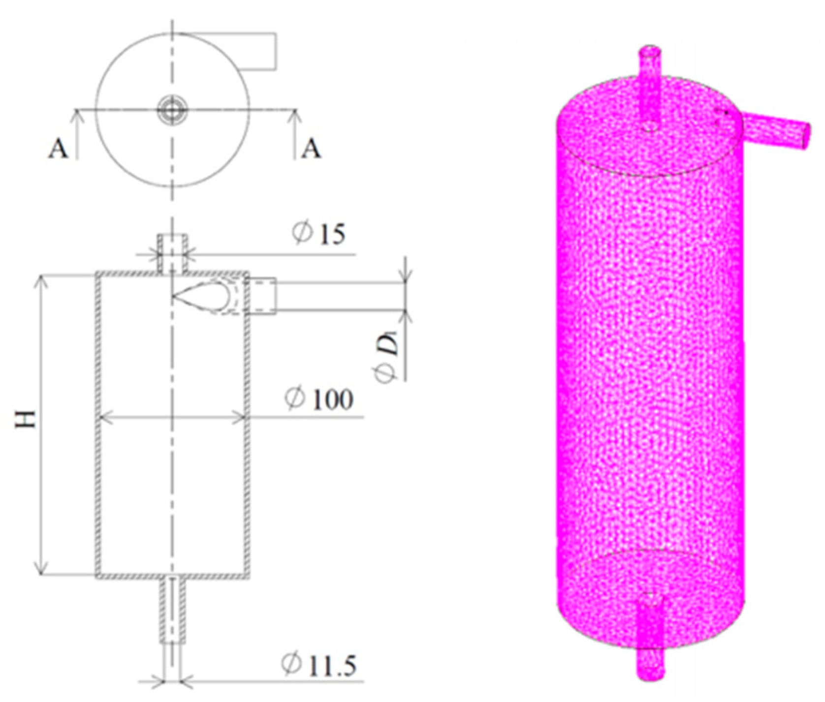
To confirm the validity of the analysis conditions and to understand the flow in the tank, fluid analysis was conducted. The fluid analysis was performed using scFLOW by Software Cradle. The schematic diagram of the tank used in the analysis and an example of mesh arrangements are shown in
Figure 3. The number of meshes was about 3 million, and the flow velocity was defined at the inlet and outlet. The VOF (volume of fluid) method was applied to analyze the free surface, and the time step was kept constant at 2.0 × 10
−4 s. In the case of swirling flow, the choice of turbulence model has a great influence on the accuracy and convergence of the analysis. Therefore, it was decided to verify the turbulence model.
As turbulence models, RANS (standard k-ε model) and DES (detached eddy simulation) were used. In DES, small vortices near the wall are computed by RANS with the standard k-ε model, and the mean field is computed by LES. In DES, the mesh near the wall, which has a large impact on the computational load, can be coarsened, and the computational load can be reduced compared to LES, so the stability of the analysis can be expected. Although LES is a good match for analyzing swirling flows, it is difficult to analyze the large aspect ratio of the mesh near the wall. As for the mesh size, RANS makes it possible to perform computation with relatively rough mesh or a large aspect ratio. On the other hand, in the regions away from walls, stable computation via LES can be carried out thanks to the fact that mesh elements can be allocated with relatively small aspect ratios. If a characteristic length scale in relation to an energy-containing eddy of a turbulent flow is longer than the representative mesh size multiplied by the DES parameter, the method switches from RANS to LES. This means that in the near-wall region, the method becomes RANS because the turbulence scale is generally small due to the small-scale eddy motion of turbulence. Therefore, the mesh was carefully divided so that only a few mm very close to the wall were analyzed with RANS, and the rest were analyzed with DES.
The accuracy of the analysis depends on the mesh size, not only for DES but also for RANS. Therefore, we set the average mesh size to 1, 3, and 5 mm and compared the analysis results. The results showed that the analysis results for 1 and 3 mm were almost identical, so the average mesh size was set to 3 mm, taking computational cost into consideration. In DES and LES, the accuracy of the discretization is crucial. The blending scheme of first-order upwind and second-order central difference schemes is applied to the advection term. The blending ratio can be controlled by the Gamma limiter at the individual cell faces. For the time derivative term, the second-order implicit scheme was applied.
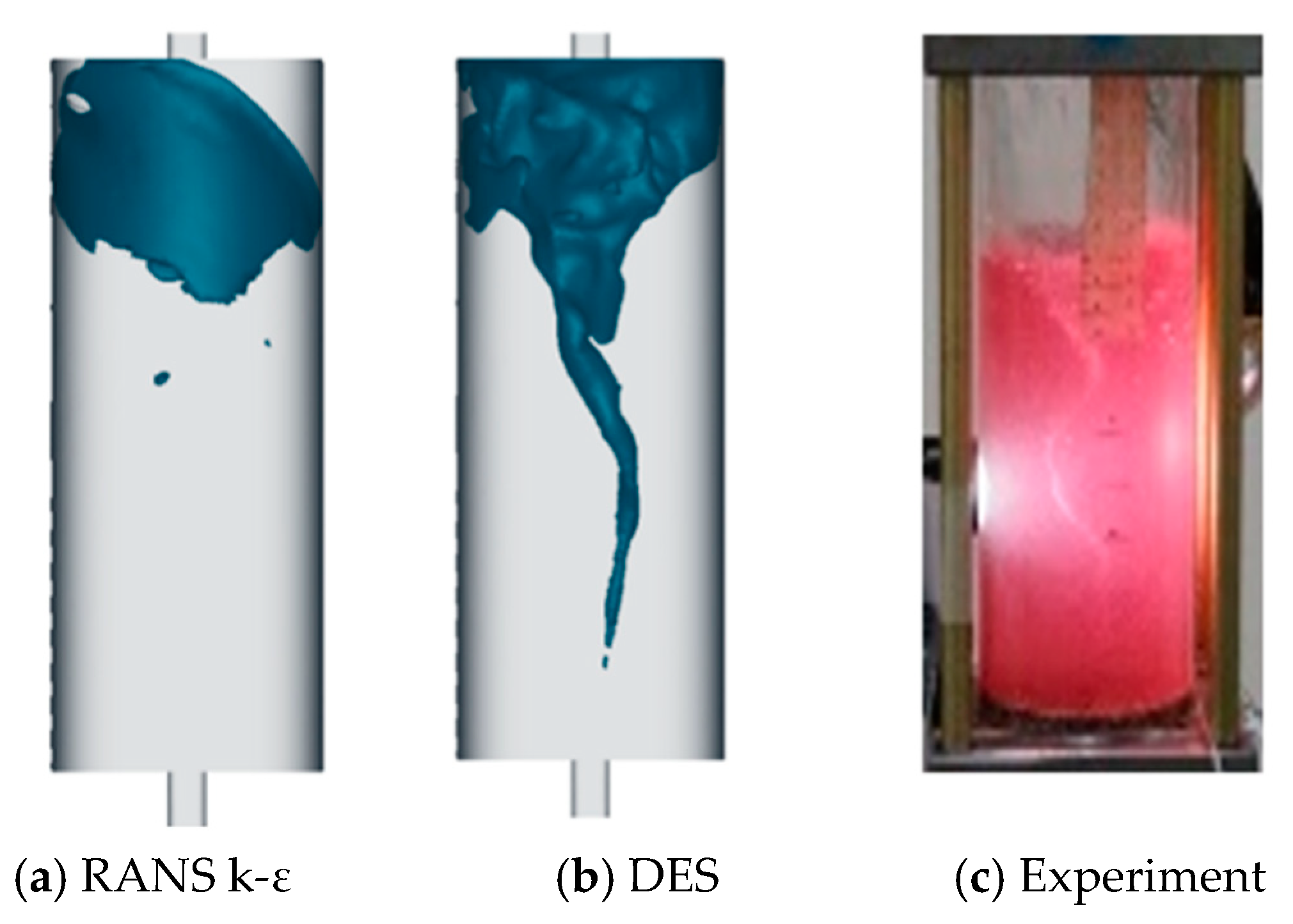
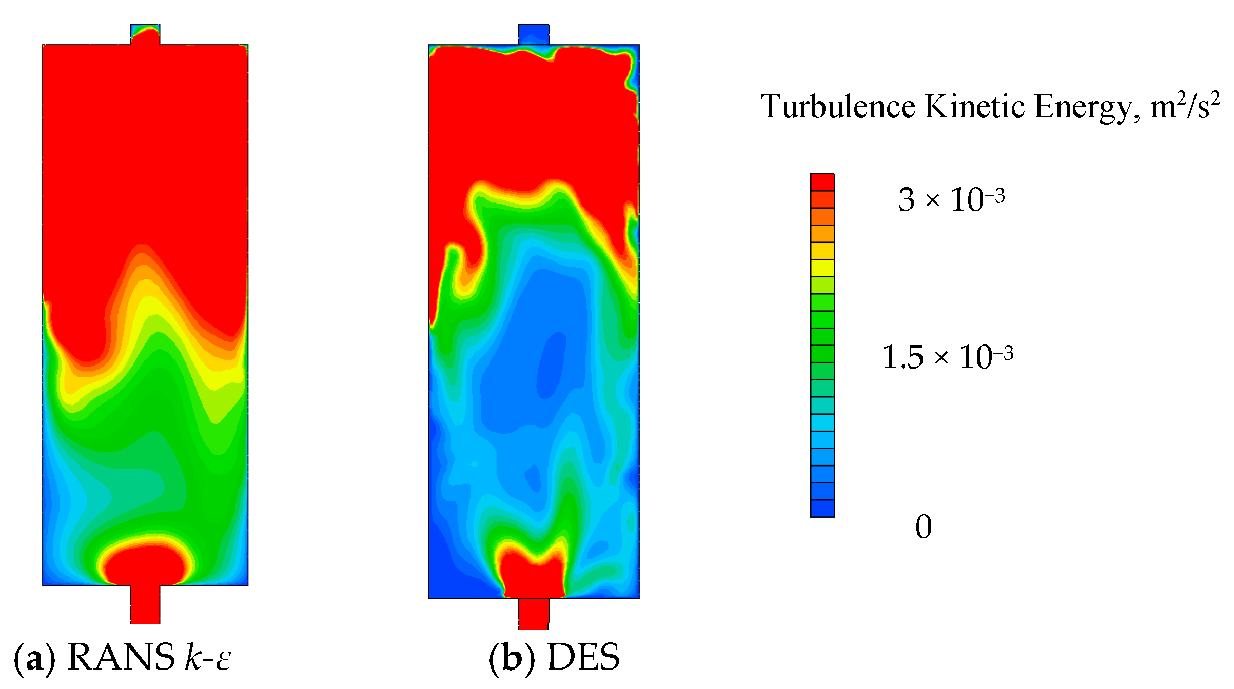
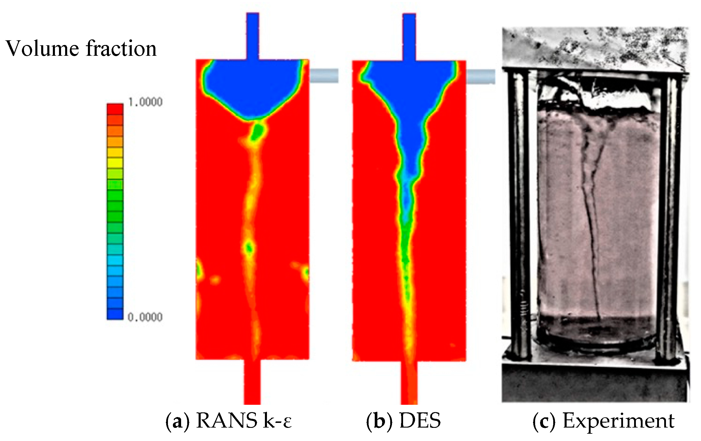
Two types of fluid, air and oil, are present in the oil tank, and the height of the air layer was set to 50 mm as the initial condition. As an example of the results of the analysis, a contour plot of the oil volume fraction compared to the results of two different visualization experiments is shown in
Figure 4. From this figure, it can be seen that a significant difference exists in the reproducibility of the swirl flow between DES and RANS, and the analysis with DES shows a good agreement with the results of the visualization experiments. The time required for the analysis was about 100 h for DES compared to about 20 h for RANS
k-
ε on a Core i9 CPU. DES analysis can perform CAE analysis of swirl flow with high accuracy, but it requires a large amount of analysis time. On the other hand, RANS analysis, which is advantageous in terms of analysis time, cannot adequately reproduce the interface, so DES was used in the following CAE analysis.
The same cyclic acceleration as in the experiment was added to the oil tank in CAE.
Figure 5 shows the comparison of the results of this acceleration-added analysis with the experimental results. The results show that RANS was not able to reproduce the shape of the liquid surface, while DES was able to reproduce the undulation of the vortex caused by the cyclic acceleration. In this CAE analysis, the CAE analysis was advanced to some extent using RANS, and the restart data was used for the DES analysis. The reason for using the RANS restart data is that when oil flows into an inlet pipe filled with air in the initial condition, a sudden pressure change occurs, and there is a high possibility that the calculations will diverge during the iterative calculation process. The results in
Figure 5 show that no vortex formation was observed in RANS, but by applying DES, the developed vortex can simulate a vortex swell due to the lateral acceleration. Therefore, RANS restart data were used as the initial condition to prevent sudden pressure changes and thus suppress divergence in the calculation.
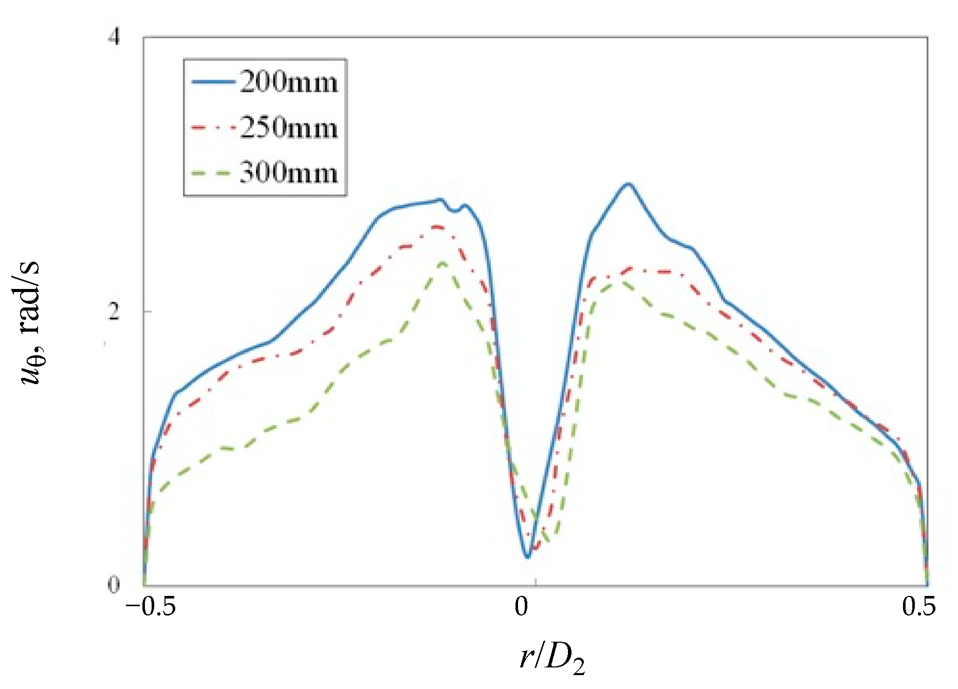
Figure 6 shows the turbulent kinetic energy in RANS and DES. The results show that the DES results were smaller than the RANS results. This means that much of the energy is considered a component of unsteady motion.
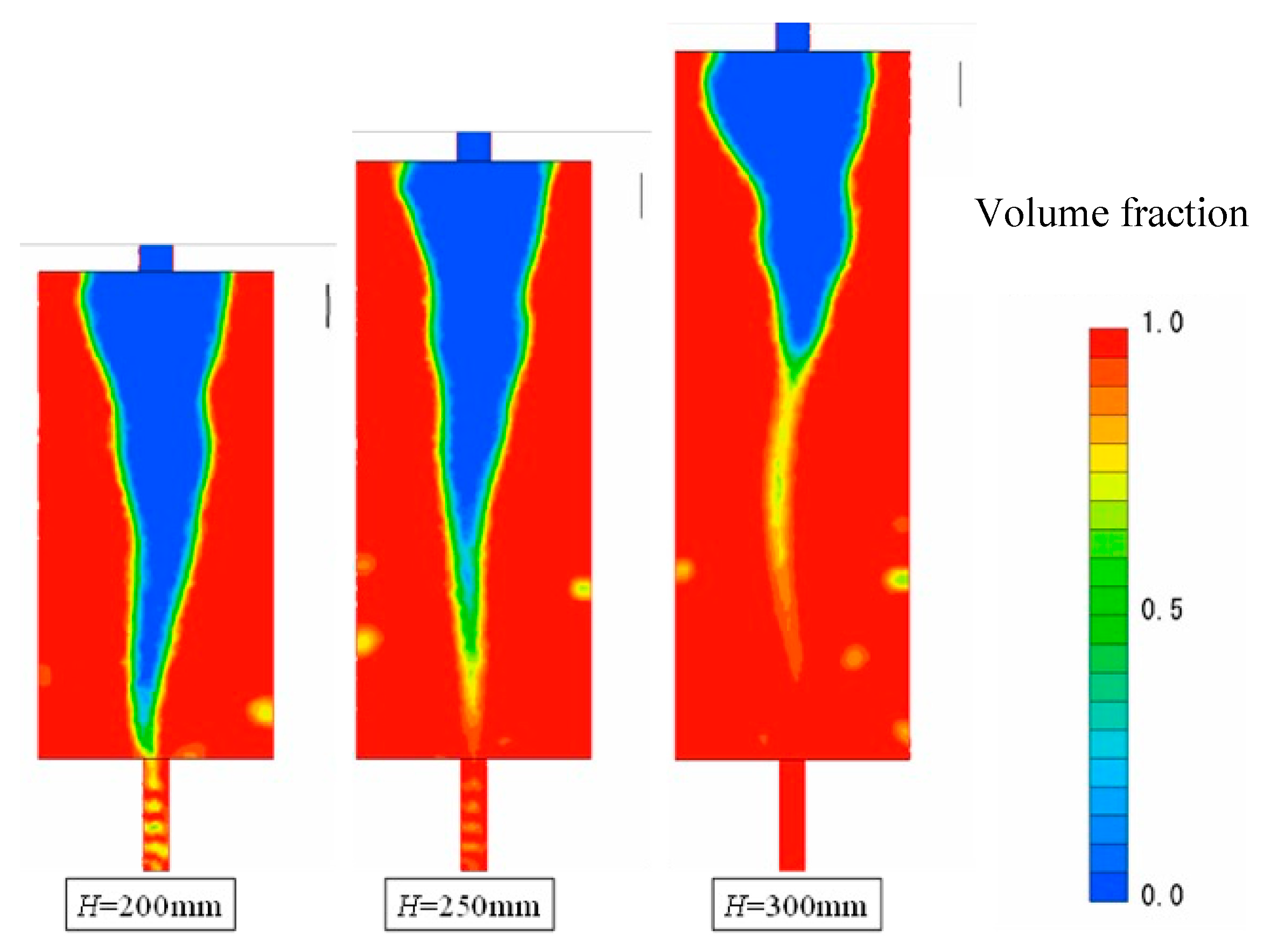
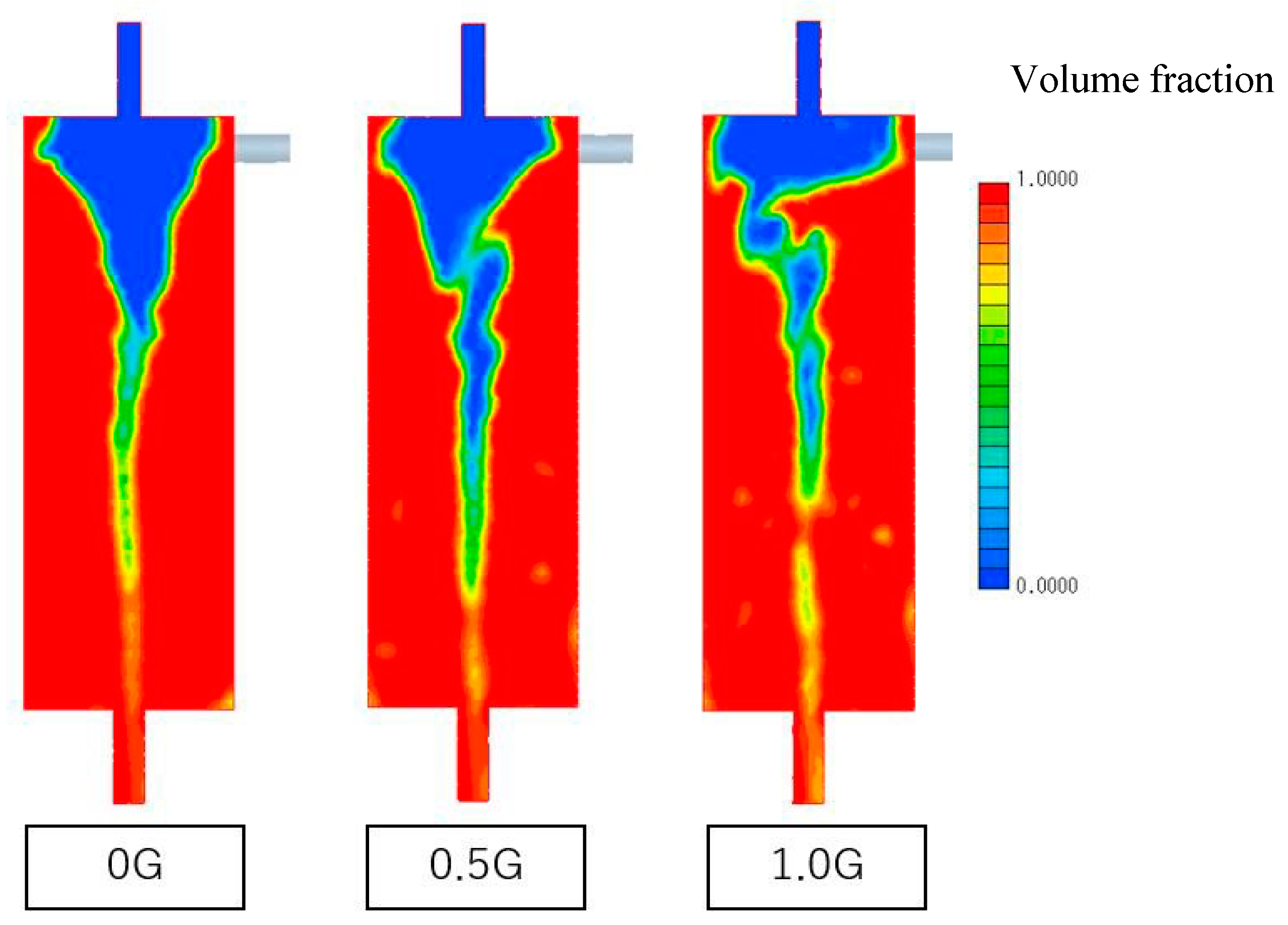
4. Effect of Lateral Acceleration on Gas–Liquid Separation Performance
In actual vehicles, lateral acceleration is often added to the separation of oil and air. Therefore, the effect of lateral acceleration on gas–liquid separation performance was investigated in consideration of engine operation. The lateral acceleration was set to 0.5 G (4.90 m/s
2) and 1.0 G (9.81 m/s
2). The oil tank height,
H, was set at the standard value of 250 mm. The oil flow rate was set to 3.9 × 10
−4 m
3/s as before, and the fluid condition was set to 3.0 × 10
4 bubbles/s with a bubble diameter of 0.30 mm. The volume contours of the analysis results are shown in
Figure 13. It was found that the gas–liquid separation performance decreases as the lateral acceleration increases. As the lateral acceleration increases, the gas–liquid separation performance becomes much worse. From the 0 G version of this figure, it can be seen that the swirling flow is well-produced when no lateral acceleration is applied. However, when the lateral acceleration becomes large, the streamline becomes oblique, indicating that sufficient centrifugal force is not being obtained. When the lateral acceleration was as large as 1.0 G, a temporary collapse of the swirl flow was observed. Even in the condition where a constant 1.0 G lateral acceleration was added, the construction and collapse of the vortex were alternately observed.
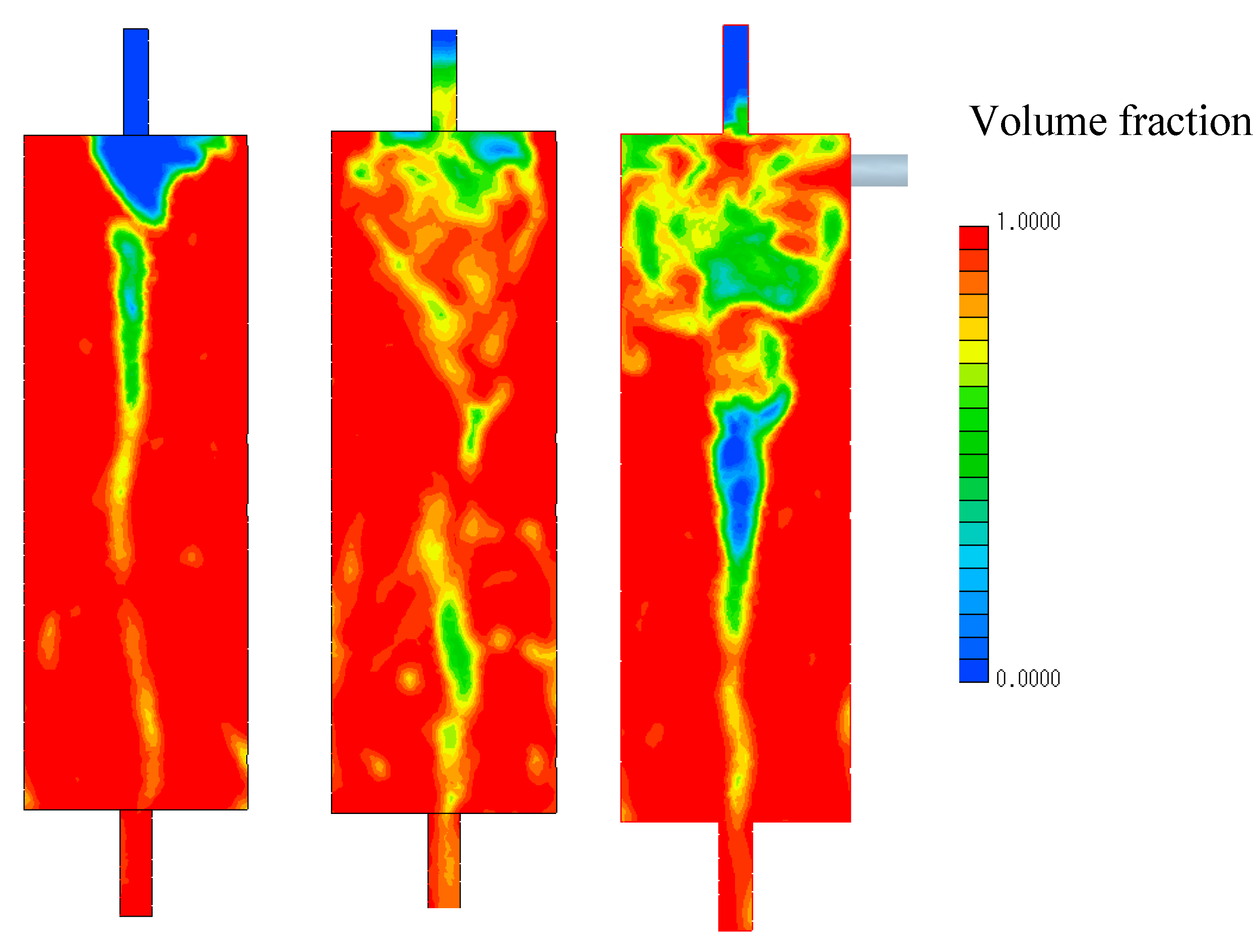
Figure 14 shows the volume contours during the vortex collapse with a lateral acceleration of 1.0 G. In other words, when a large lateral acceleration is added, the collapse and reconstruction of the vortex flow occur periodically in the oil tank, suggesting that the amount of gas flowing out increases immediately after the collapse of the vortex flow.
5. Conclusions
With the aim of improving the removal efficiency of air bubbles remaining in the hydraulic oil, we have succeeded in improving the bubble removal performance even under conditions of added acceleration by generating an appropriate swirling flow. First, an acrylic model of an oil tank was used and numerical analysis using various turbulence models was performed to confirm the accuracy. Next, the parameters of the bubble removal system, such as the size of the oil tank, were examined. Furthermore, the bubble removal performance under lateral acceleration was examined.
(1) Increasing the inflow velocity is effective in improving the gas–liquid separation performance, but if the vortex reaches the outflow pipe, both the gas rate and the number of bubbles will increase.
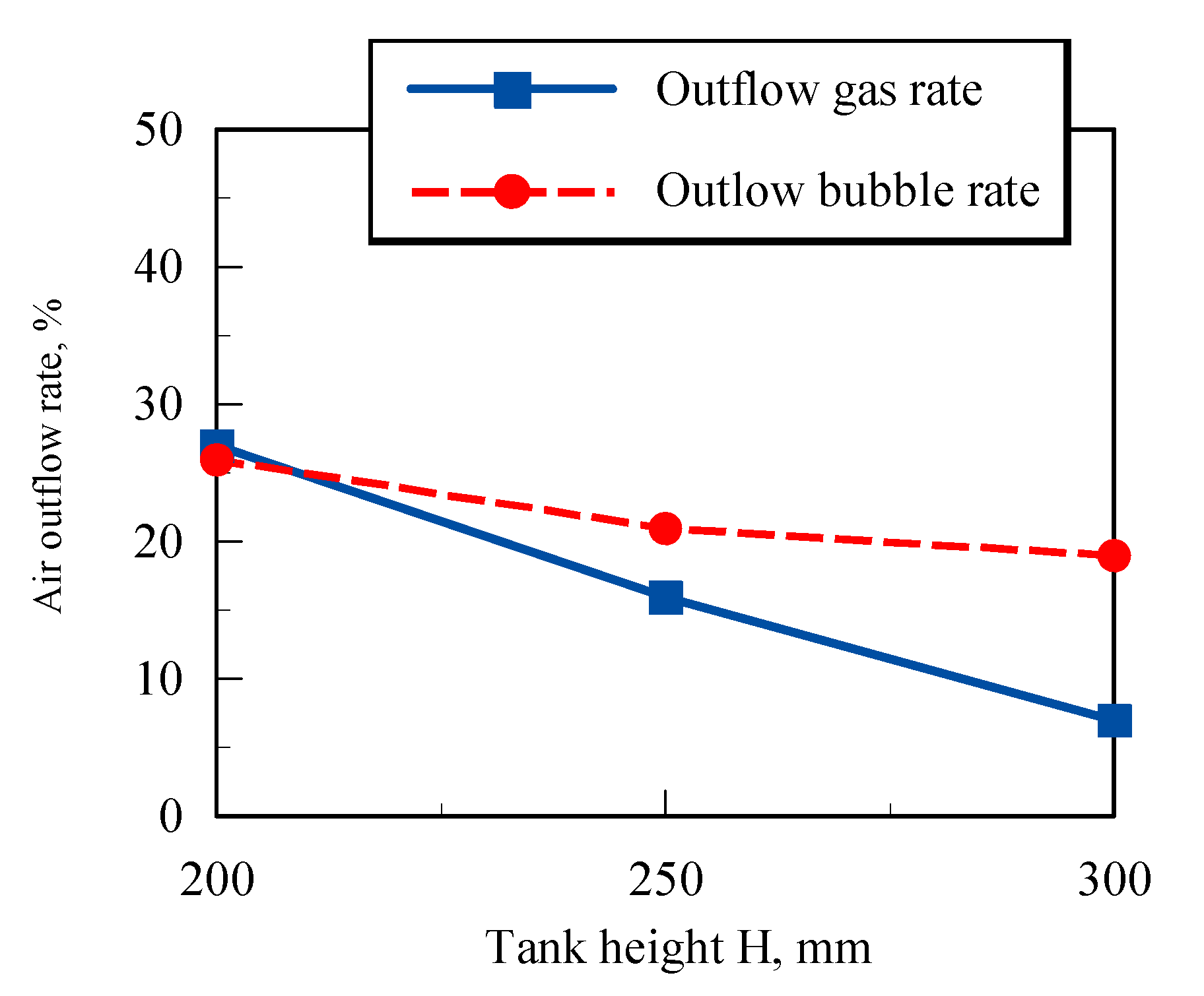
(2) It is effective to increase the tank height to improve the gas–liquid separation performance. The bubble release rate does not decrease so much even if the tank height is increased.
(3) The gas–liquid separation performance of the oil tank decreases when a large lateral acceleration occurs.


