Article

Numerical Simulation of the Effect of a Single Gust on the Flow Past a Square Cylinder

Laboratory for Innovative Environmental Technologies, School of Mechanical Engineering, National Technical University of Athens, 9 Heroon Polytechniou Street, 157 73 Zografou, Greece
*
Author to whom correspondence should be addressed.
Fluids 2022, 7(9), 303; https://doi.org/10.3390/fluids7090303
Submission received: 25 July 2022 / Revised: 6 September 2022 / Accepted: 9 September 2022 / Published: 15 September 2022

Abstract

:
The flow past a square cylinder under the influence of a one dimensional gust was investigated using computational fluid dynamics (CFD). The effect of upstream wind gusts of the same amplitude but different duration was investigated with respect to their effect on the flow, the vortex-shedding, and the pressure distribution around the square cylinder. For the computations, a very large eddy simulation (VLES) model was implemented in an in-house code and validated against numerical and experimental results from the literature. The gusts of different duration were found to have a distinctly different effect. The short-duration gust causes a lock-on behavior with cessation of the alternating vortex shedding, and a symmetric pair-vortex was created above and below the square cylinder. It was observed that the pressure distribution on the lateral sides of the cylinder has the same magnitude and phase, which resulted in a zero total lift coefficient. In terms of a free-standing structures, such as a building, this would lead to zero instantaneous forces and pressure difference in the lateral direction with obvious implications for dynamic response and cross ventilation.

1. Introduction

Turbulent and non-stationary winds are often observed in the atmosphere, having the common characteristic of different speeds at different timescales [1]. Large fluctuations in wind speed over small timescales are associated with wind gusts [2] and are of interest to several applications such as wind turbine operation, loads on structures, aeronautics [3,4], and rail transport [5].
Most studies of wind-induced gusts have been experimental ones that measured the flow characteristics in, e.g., urban environments throughout the world, such as Newcastle, Australia [6], or Shangai and Shenzen, China [7,8]. Focus is usually placed on the yet-to-be well-understood urban flow physics [7,8] but also on the characterization of the gust itself [6]. Even outside urban areas, research into the meteorological physics of the gusts is active for local phenomena such as the Vento Norte in Southern Brazil [9] or coastal areas, e.g., Lake Victoria [10] or Pearl River Estuary [11]. Yet another active area of research is extreme gust phenomena such as typhoons [12,13] or tropical cyclones [14]. Numerical studies are not as widespread, and most concern wind turbine operation during wind gusts. Researchers have found ways to reduce loads exerted on wind turbines [15,16] and to make them as efficient as possible when they are subjected to extreme gusts by designing and tuning fuzzy logic controllers [17] and optimizing the design of the wind turbine blades [18,19].
On the other hand, only a limited number of numerical studies of an unsteady, gusty flow past a bluff body have been published. Some examples are a sinusoidal signal past a circular cylinder [20] or a single coherent gust past a flat plate [21], while other studies have used gust inlet velocities that describe a sequence of gusts [22], possibly even of a stochastic nature [23,24], and are more similar to oscillation functions than to a single gust described by U.S. weather-observing practice [25].The most common design standards prescribed to provide guidelines in order to take wind gusts into account and to satisfy U.S. weather-observing practice [25] are Kasperski’s standard [26] and the standard defined by the International Electrotechnical Commission (IEC) 61400.2-2013 [27]. The latter describes the extreme operating gust (EOG), which is a representative gust profile forming a symmetric Mexican hat shape. This standard is used to describe the gust for a wind turbine during its operation, and this is probably the reason that it has not been used to describe gusts to which bluff bodies are subjected [28].
Turbulent flow past bluff bodies has attracted significant attention in recent years, with a cylinder of square cross section being one of the most common geometries studied, where vortex shedding, flow separation, and shear-layer instability appear in the vicinity of the bluff body [29]. The flow past a square cylinder may be considered relevant to many engineering applications such as modern buildings, towers, high-rise skyscrapers, and vertical columns of long-span bridges because they share similar aerodynamic characteristics [30]. Many studies have been carried out for this type of flow, investigating wake vortex dynamics [31], the interaction with the ground [32], dependence on Reynolds number [33], the effects of 3D flow structures [34], a universal Strouhal number [35], and vortex-shedding suppression [36].
The complex flow separation, vortex-shedding, and recirculation zones on and in the wake of the square cylinder may induce large instantaneous aerodynamic forces, and the investigation of the drag and lift forces exerted on its external surfaces provides important information for numerous applications. One of the less investigated applications in this context is that of the operation and energy performance of a building and of occupant comfort (natural ventilation, infiltration, wind loads), in spite of its obvious dependence on the pressures exerted on the outer surfaces. It is well-established that infiltration and ventilation is a crucial factor when it comes to sustainable energy buildings [37] and healthy environments [38], and many relevant studies have been carried out regarding the impact of opening positions [39], the effect of neighboring objects [40], and also the accuracy of applied numerical methodologies [41].
However, to the authors’ knowledge, the effect of single, instantaneous fluctuations such as gusts in upstream conditions has not been extensively investigated until now. Thus, the novel aim of the present numerical study is to introduce a realistic wind gust, which satisfies the IEC Standard [27] and U.S. weather-observing practice [25], upstream of the flow past a square cylinder and to compare the results for gusts of varying duration.
Although there are many experimental studies of the flow past a square cylinder conducted, e.g., by measuring static pressure distributions at midspan in a wind tunnel [42] or by directly measuring aerodynamic coefficients in wind tunnel [43] and water channel tests [44,45], the numerical simulation of this flow is challenging. Several numerical studies have been performed using and comparing RANS, URANS, and LES turbulence models [46,47,48,49], with attempts to perform DNS being much less common [50] even if considerably old [51]. Recently, hybrid RANS/LES methodologies have appeared, i.e., DES [52], VLES [53], and PANS [54], which are significantly more attractive in terms of demands on computational resources compared to DNS and LES and may provide a better representation of unsteady turbulent flows than URANS. For the present study, the Han and Krajnovic [55] VLES model is implemented in an in-house code. The implementation is validated against the measurements of Lyn et al. [45] for the steady flow past a square cylinder at Re = 22,000 in order to reliably apply it to studying the effects of upstream gusts. After validation of the code, single gust events are applied to the inlet boundary of this flow, and the effects of two cases of different gust duration are compared. It is found that although the two gust events have the same velocity structure with a different duration, and they both induce high instantaneous pressures on the cylinder’s outer surfaces, their effect on the global indices such as lift, drag, or pressure differences are markedly different. Implications to infiltration and ventilation of buildings are discussed.

2. Materials and Methods

2.1. Numerical Code

The methodology applied in the in-house code for the numerical computation of the flow field solves the Navier–Stokes equations using the finite-volume method. The generalized form of the governing equations is
t ( ρ Φ ) + x ( ρ u Φ ) + y ( ρ v Φ ) + z ( ρ w Φ ) x ( Γ Φ Φ x ) y ( Γ Φ Φ y ) z ( Γ Φ Φ z ) = S Φ
where u, v, and w are the corresponding velocity components in local Cartesian coordinates, and ρ is the density of the fluid. Φ is a generalized variable that takes values Φ = 1, u, v, and w for the continuity and momentum equations, respectively, or Φ = k,ε for the conservation equation of turbulent kinetic energy (k) or its dissipation rate (ε), respectively. For the continuity equation, SΦ in (1) is zero, while for the momentum equations, it is written in tensor form as:
S Φ = u i = Ρ x i + x j μ u j x i
where xi is equal to x, y, z and ui to u, v, w when i is 1, 2, 3 respectively. In addition, for the k and ε conservation equations, the source term SΦ is:
S Φ = k = μ u i x j u i x j + u j x i ρ ε
S Φ = ε = c 1 ε k u i x j u i x j + u j x i c 2 ρ ε 2 k
In Equations (1)–(4), the other variables appearing are ΓΦ = μ/σΦ, μ = μl + μt, where μl is the dynamic viscosity of air, and μt is the turbulent viscosity, with μt = Cμk/ε for the standard k-ε turbulence model. In addition, constants are c1 = 1.44, c2 = 1.92, cμ = 0.09, σui = 1, σk = 0.9, and σε = 1.3.
The code is a standard finite volume implementation of the SIMPLE algorithm [56] on a Cartesian grid with collocated variables and the discretized equations are solved using a tri-diagonal matrix algorithm (TDMA). For the convective terms, the bounded second-order upwind scheme (BSOU) [57] is used, which combines and bounds the first- and second-order upwind schemes, providing better accuracy than the hybrid scheme and reducing the numerical diffusion problems. Previous application of this CFD model to steady state external flows past buildings and urban geometries has proven reliable [58,59,60].
For turbulence closure, we apply the Han and Krajnovic [55] VLES concept with the k-ε model, where the resolution control function, Fr, was bounded between zero and one:
F r = min 1.0 , 1.0 exp ( β L c L k ) 1.0 exp ( β L i L k ) n
Lc, Li, and LK are the turbulent cut off length scale, integral length scale, and Kolmogorov length scale, respectively, defined as:
L i = k 1.5 / ε L c = C x ( Δ x Δ y Δ z ) 1 3 L Κ = v 3 / ε 1 / 4
In Equation (6), the model constants are Cx = 0.61 and n = 2, and the recommended value of β is β = 2 × 10⁻³ based on the numerical studies in the original Speziale VLES model [53]. It should be noted that near the wall, Lc > Li, leading to Fr→1 (see Equation (5)), so the hybrid model recovers to the RANS model, a behavior similar to the (detached eddy simulation) DES concept [52].
Turbulent viscosity from the k-ε model is calculated as:
μ t s u b = F r ρ C μ k 2 ε

2.2. The Flow Field Past a Square Cylinder

Validation is performed for the flow past a square cylinder according to the experiment of Lyn et al. [45]. At Re = 22,000, with air at atmospheric pressure and standard temperature, the cylinder edge length was chosen to be D = 1 m on the XY plane (Figure 1a), the height of the square cylinder is parallel to the z-axis, and the direction of the flow is along the x-axis with an inlet velocity of Uinlet = 0.33 m·s−1.The computational domain is 20D × 14D × 4D, and the center of mass of the square cylinder is at (x,y) = (0,0) (Figure 1a). No-slip wall boundaries simulate the water tunnel in the lateral direction, and free-slip boundaries were assumed for the top and bottom of the domain in the spanwise direction. Zero gradient boundary conditions were imposed at the outflow, which was 15D away from the rod center, and no pressure reflections were observed. In this paper, the flow was examined with a mesh (Figure 1b) that consists of 0.378 million cells (M378) in total. This is similar to the coarsest (M1) mesh that Han and Krajnovic used and found to be sufficient. The grid is clustered near the wall, and the first node is located at Δy/D = 2.5 × 10⁻³. In the present study, grid independency was also investigated with a finer mesh (M575), which consisted of 0.575 million cells. Further details on the performance of the numerical setup are presented in Section 3.1.
The non-dimensional time step Δt* = Δt/(D/Uinlet) is equal to 0.11. At the inlet, the mean horizontal velocity U is uniform and follows the horizontal direction, the turbulent intensity is set to 2%, and the turbulent viscosity ratio is equal to 20.0.

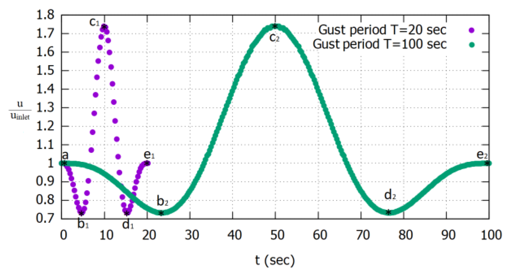
2.3. Gust Introduction

According to U.S. weather-observing practice [25], a gust is a sudden, brief increase in the speed of the wind, which lasts less than 20 s. The peak of the wind speed should reach at least 16 knots, and the variation in wind speed between the peaks and lulls should be at least 9 knots [25]. Although gusts of shorter duration (~3–5 s) are most common, gusty turbulent fluctuations may also last in the order of minutes [61] also in complex terrain [62].
For numerical simulation, some form of gust function must be applied to the inlet velocity profile of the above-mentioned flow field. Standardization of gust definition has been performed by IEC work groups, and one of the extreme wind conditions, described by the International Electrotechnical Commission (IEC) standard IEC 61400.2-2013 [27], is the extreme operating gust (EOG). This representative gust profile agrees with gust events that were found to occur 100 times during a 12 month interval [6,27] and takes on the form of a symmetric Mexican hat shape with a decrease in speed followed by a steep rise, a steep drop, and a rise back to the original value. The IEC standard is usually applied to describe the gust for a wind turbine in operation, but in the present study, it was also considered valid in order to define the gust velocity profile upstream of the bluff body being studied:
u ( t ) = u ( z ) u ( z ) 0.37 V g u s t N sin 3 π t T ( 1 cos 2 π t T u ( z ) t < 0 0 t T t > T
In Equation (8), a normal steady-state profile u(z) is assumed to persist up to t = 0 s when the gust begins. The gust period is the total event duration, considered to be T = 10.5 s for a recurrence period of N = 1, and VgustN is the gust amplitude at the hub height, which is the height of interest in the case of a wind turbine [6]:
V g u s t N = β σ 1 1 + 0.1 D Λ 1 Λ 1 = 0.7 z h u b 21   m w h e n w h e n z h u b < 30   m z h u b 30   m σ 1 = Ι 15 15 + α V h u b α + 1
where Λ1 is the turbulence scale parameter, β = 4.8 is the parameter for the EOG model when N = 1, D = 5 m is the rotor diameter, and σ1 is the standard deviation. I15 = 0.18 is the dimensionless characteristic value of the turbulence intensity at 15 m/s, and α = 2 is the dimensionless slope parameter for a class III SWT. Here, Vhub is considered to be the inlet mean horizontal velocity.
The gust function and parameters in Equation (8) refer to a full-scale velocity profile and gust period (Tn). For the present situation, this may be reasonably considered to correspond, e.g., to a full-sized square cylinder (e.g., building structure) of side Ln = 10 m and an upstream wind velocity of un = 6.3 m/s. In order to facilitate comparison with the results of the steady upstream velocity validation test presented above, the gust function should be scaled and a corresponding gust period (Tm) be calculated. Based on standard scaling procedures [63], we can define a time-scale similarity ratio between fullscale and validation (model) scale:
T m T n = L m u m L n u n = 1.9
In the validation test case, the square cylinder had a side length of Lm = 1 m, and the inlet streamwise velocity was um = 0.33 m/s. Thus, if the full-scale gust period is Tn = 10.5 s (in agreement with the standard of EOG [27]), then the gust period of the model square cylinder would be Tm ≈ 20 s. From Equations (8) and (9), the model gust velocity signal is calculated and presented in Figure 2. The same Figure also shows a wind gust of the same amplitude but an arbitrarily exaggerated model scale duration of 100 s, corresponding to a full-scale gust period (Equation (10)) of 52 s (a little less than one minute), which was also examined for comparison purposes.

3. Results and Discussion

Validation of the VLES implementation in the code was performed by comparison to results from the literature, and then, the gust events described previously were introduced to the upstream flow and the flow field around the cylinder, and the pressure distribution on its outer surfaces were calculated.

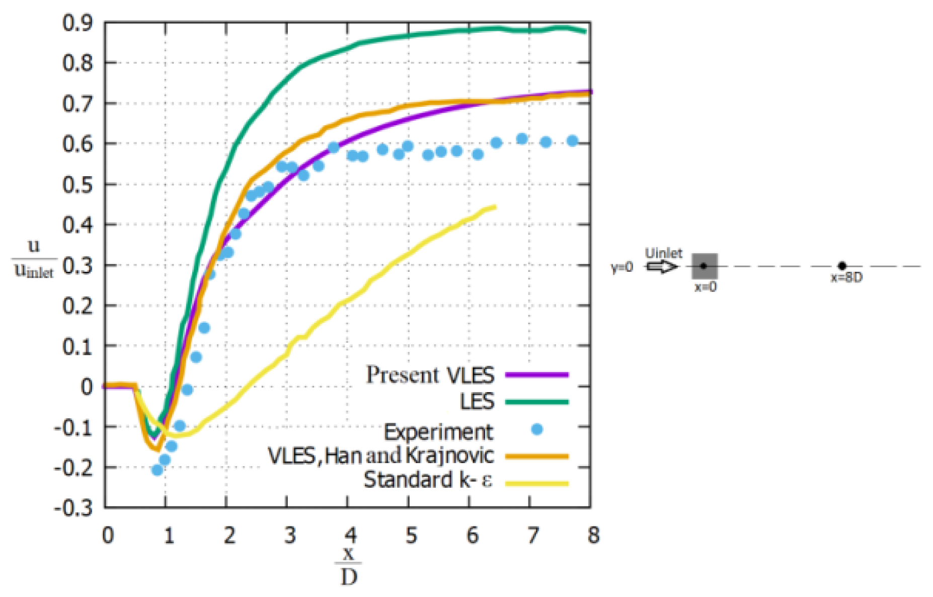
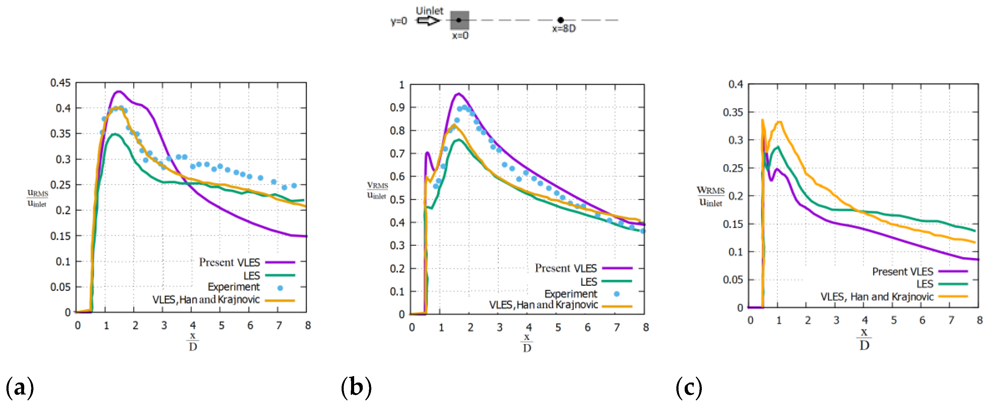
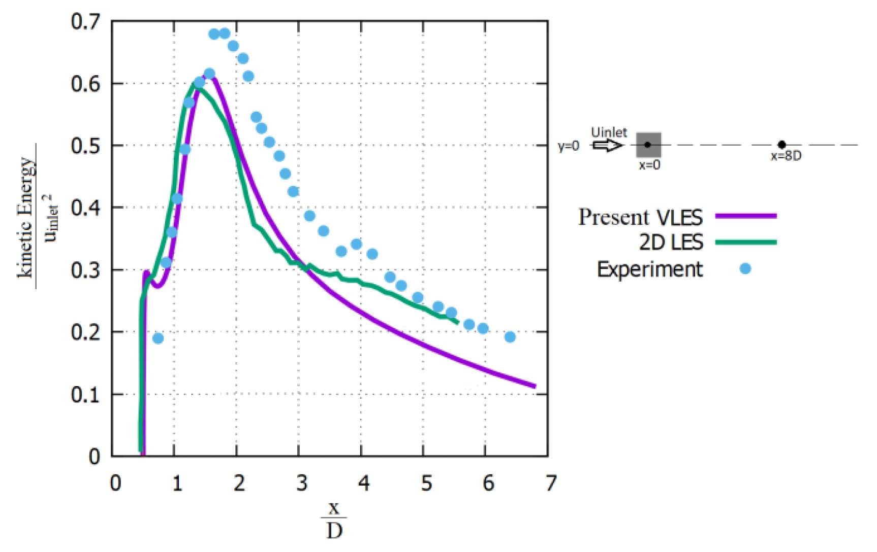
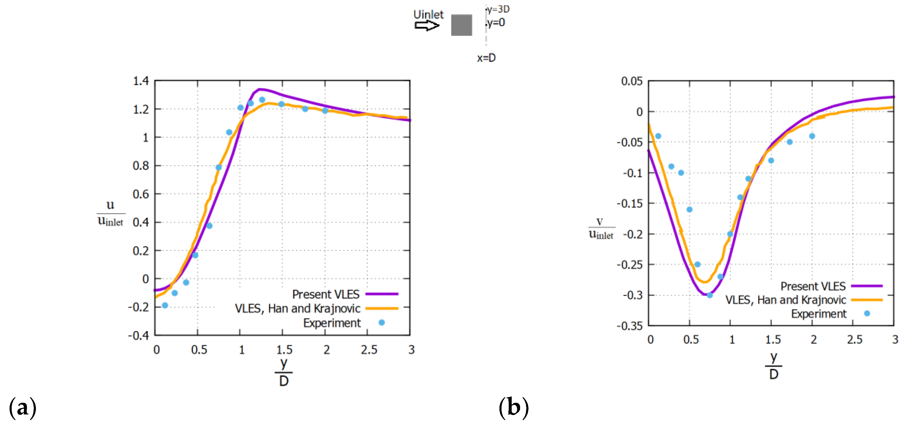
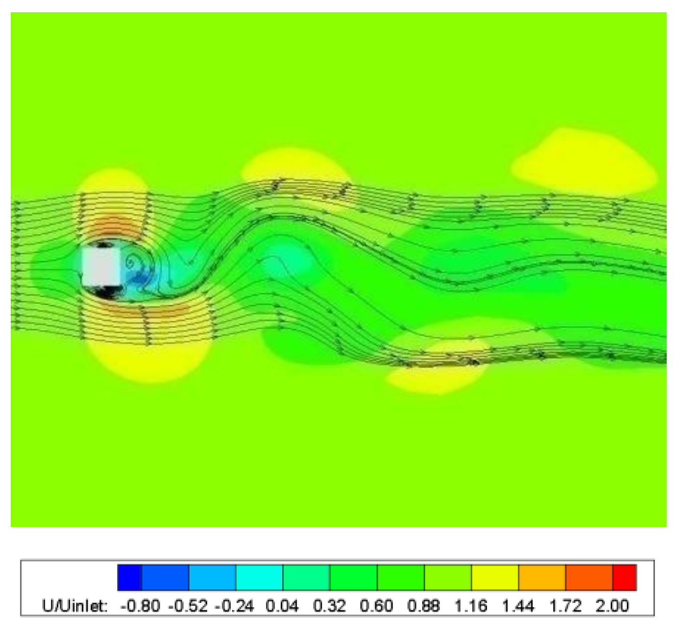
3.1. VLES Validation of Flow Past a Square Cylinder

Validation of the VLES implementation in the in-house code was performed by comparison to the experimental measurements of Lyn et al. [45] and the numerical calculation of Han and Krajnovic [55] for the turbulent flow past a square cylinder. The computational domain and the boundary conditions have already been discussed in Section 2.2. However, for the study of the wind gusts, it was also necessary to examine this flow when free-stream boundary conditions are imposed in the lateral direction instead of the wall boundaries present in the water channel realization.
Calculation results of some of the flow field global parameters are presented in Table 1 and compared with previous studies, and grid independency is also verified. Similar mean and RMS drag and lift coefficients are computed with theM378 and M575 meshes, giving a maximum deviation of ~2% for <CD>.
Minimal deviations are observed when free-slip and no-slip boundaries were set, and overall, the results are in agreement with those of other studies given the rather large spread in those results. An exception is the standard deviation of the lift coefficient, which is close only to the lift coefficient computed with the denser grid by Han and Krajnovic VLES [55]. It has to be mentioned that the precise grid distribution of the meshes in other studies is not known. Given the level of agreement and the spread in the results among other studies, it has been considered that mesh M378 is adequate, and all the calculations below are performed on this mesh.
In Figure 3, the timeseries of the streamwise velocity component at the centerline, five cylinder side lengths downstream (x/D = 5), is shown for 234 non-dimensional time units, which correspond to ~30 complete natural shedding periods. The frequency of these periods gives a Strouhal number equal to St = f.D/Uinlet = 0.122, which is the same as the value calculated in [55].
In terms of the behavior of the turbulence modeling, the mean y+ values of the first node along the square cylinder sides are presented in Figure 4 and shown to fall within the range of y+ = 1 − 4.5. Figure 5 shows the ratio of the effective to laminar viscosity as an indication of the performance of the VLES model. Effective viscosity is limited to an order of magnitude increase compared to laminar viscosity, mainly in areas of high shear (shear layers from cylinder sides and vortex cores), but for the most part of the flow, the increase is about fivefold compared to orders of magnitude commonly found in URANS studies.
The mean flow field is computed for the above-mentioned duration of 234 non-dimensional time units and the mean streamwise velocity profile along the centerline behind the cylinder is presented in Figure 6. Results of the present study are in good agreement with Lyn et al.’s experiment [45] and also agree with those of Han and Krajnovic [55], with a small divergence of the order of 4% far downstream, where RANS behavior is recovered, and grid spatial resolution is coarser. Franke and Rodi’s [64] calculation using the standard k-ε model shows an unrealistically large recirculation zone, while Sohankar and Davidson’s LES [47], also shown for comparison, overestimated flow recovery in the wake.
The profiles of the three fluctuating (RMS) resolved velocity components along the central line of the wake are shown in Figure 7. The uRMS velocity is in good agreement with both the experimental measurements and Han and Krajnovic’s VLES [55] within the recirculation zone behind the cylinder but fails to predict the behavior in the far wake. However, the vRMS velocity component is in excellent agreement with the experimental measurements, while it was underestimated by Han and Krajnovic’s VLES [55] and LES [47]. This should also be considered in relation to the higher RMS value of the lift coefficient in Table 1. Experimental data were not available for the wRMS velocity component, but the predictions of the models are generally in close agreement to each other. Total fluctuation energy (TFE) calculated along the central line of the wake is shown in Figure 8. The total fluctuation energy is computed from the three fluctuating resolved velocity components as TFE = ( u 2 ¯ + v 2 ¯ + w 2 ¯ )/2 and is compared to Lyn et al.’s experiment [45] and to Bouris and Bergeles’s 2D LES results [65]. Finally, present VLES is in good agreement with the experimental measurements within the recirculation zone and the near wake, but the effect of the uRMS velocity deviations observed in Figure 7 becomes evident in TFE in the far wake, i.e., downstream of x = 3D.
Mean velocity profiles in the transverse direction at x/D = 1 are presented in Figure 9. It is verified that in the near wake, both mean streamwise and transverse velocity profiles are in good agreement with the experiment.
Furthermore, streamlines of the average flow are presented in Figure 10 and agree well with the results of Trias et al. [50], who conducted a DNS study past a square cylinder at Re = 22,000. The two large recirculation zones appearing at the top and leeward sides of the cylinder (Figure 10) are of the same overall size as those predicted by the DNS method [50] even though the smaller recirculation zone appearing [50] near the leeward corner is not predicted here.
Furthermore, instantaneous streamlines that correspond to time instants 1/20, 5/20, 9/20, 11/20, 15/20, and 19/20 of the period (τ) of vortex shedding are shown in Figure 11. These streamlines are in a good agreement with the streamlines computed with the Launder and Sharma low-Re k-ε model by Raisee et al. [66].

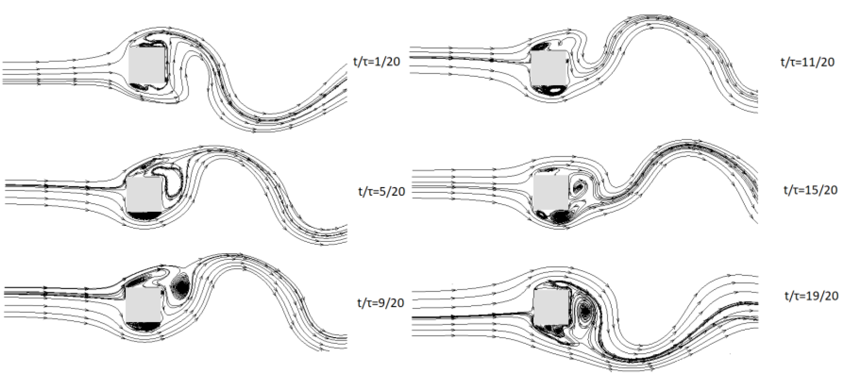
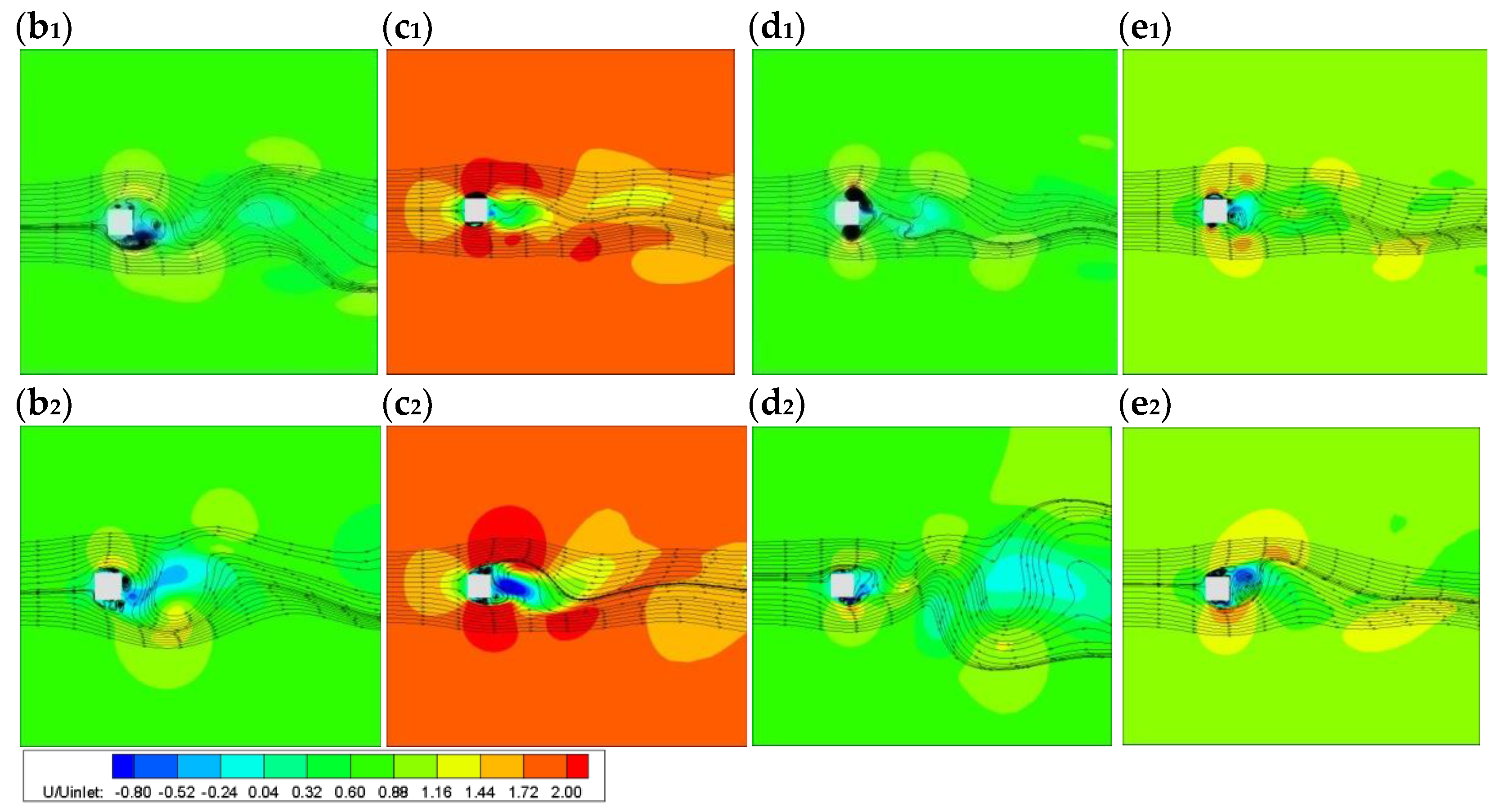
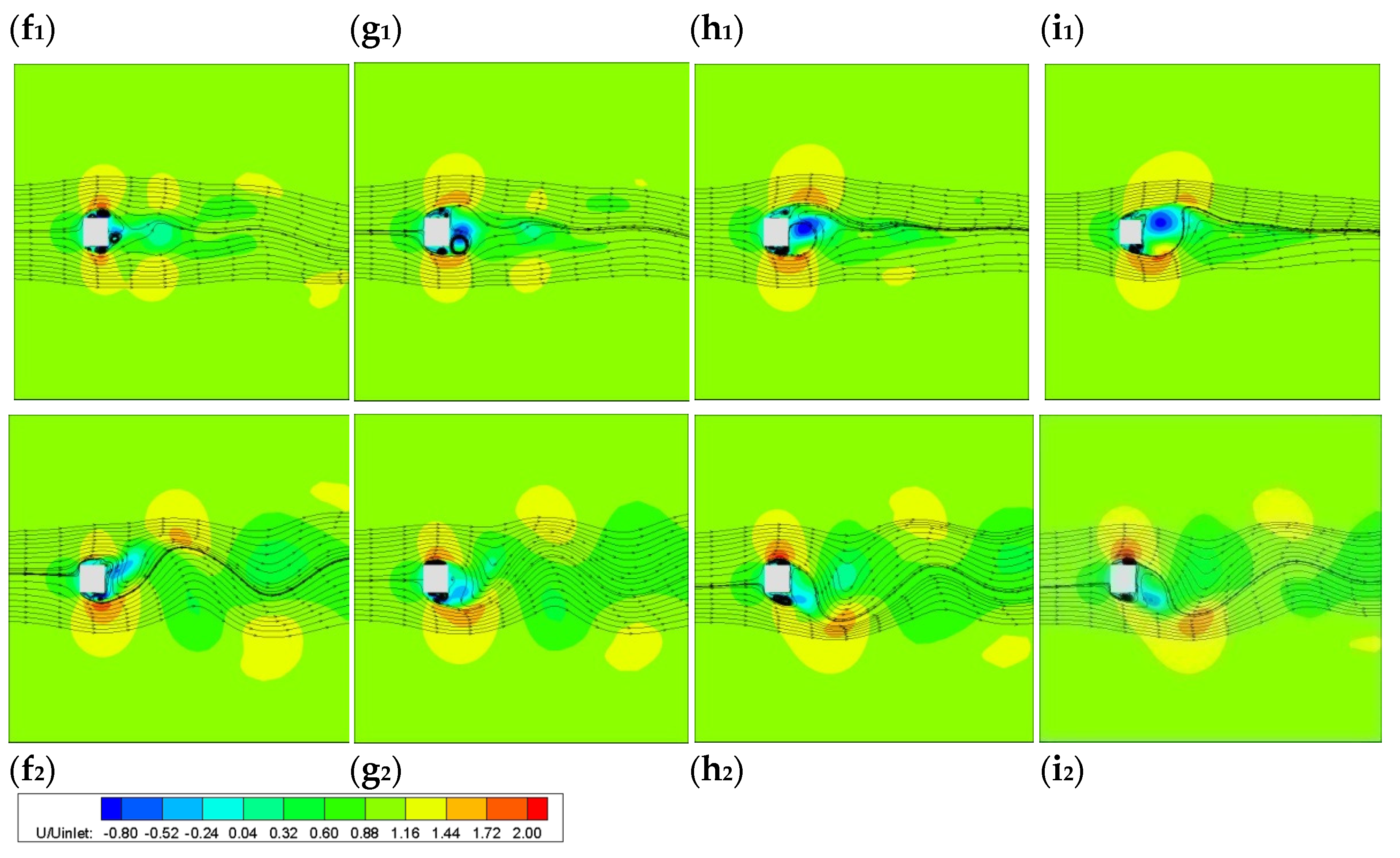
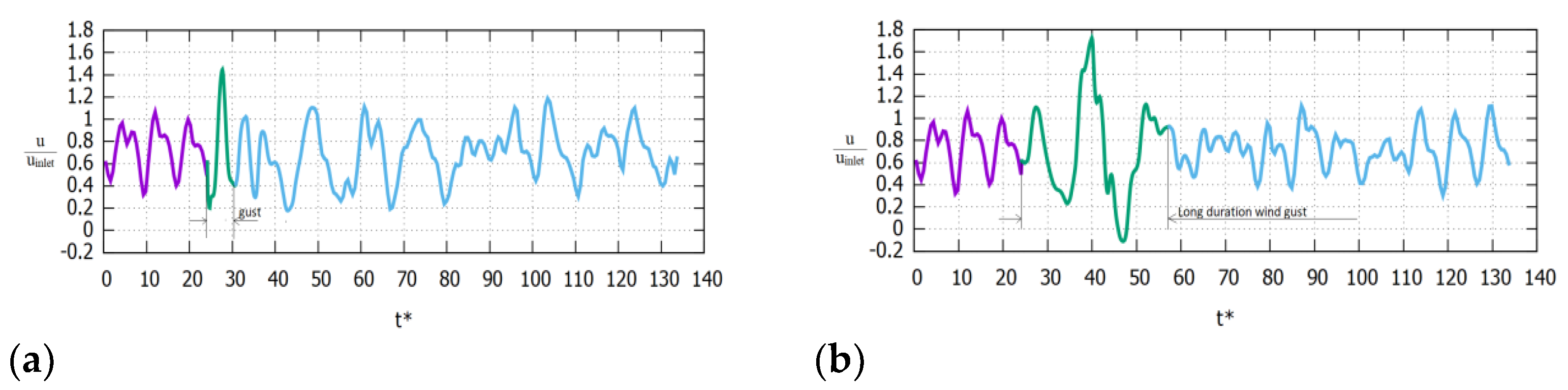
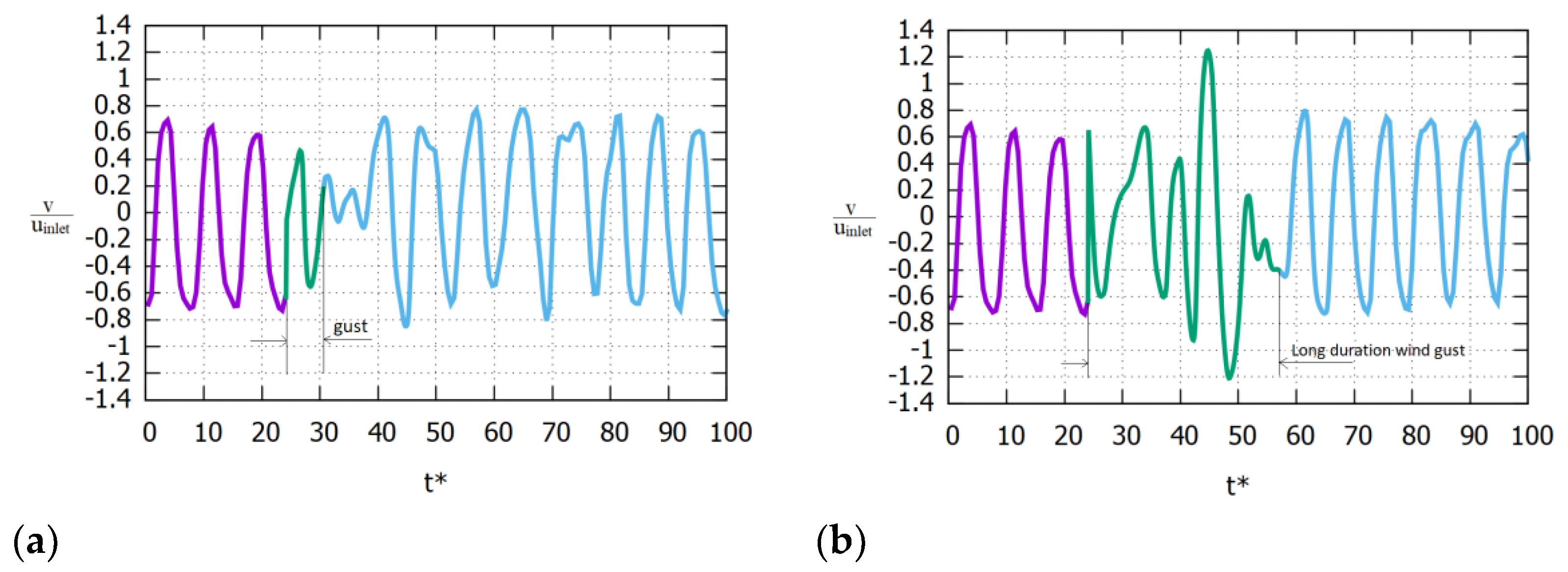
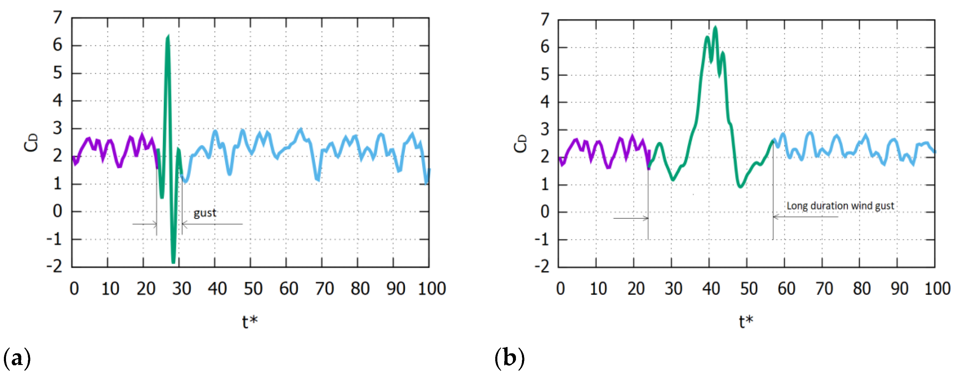
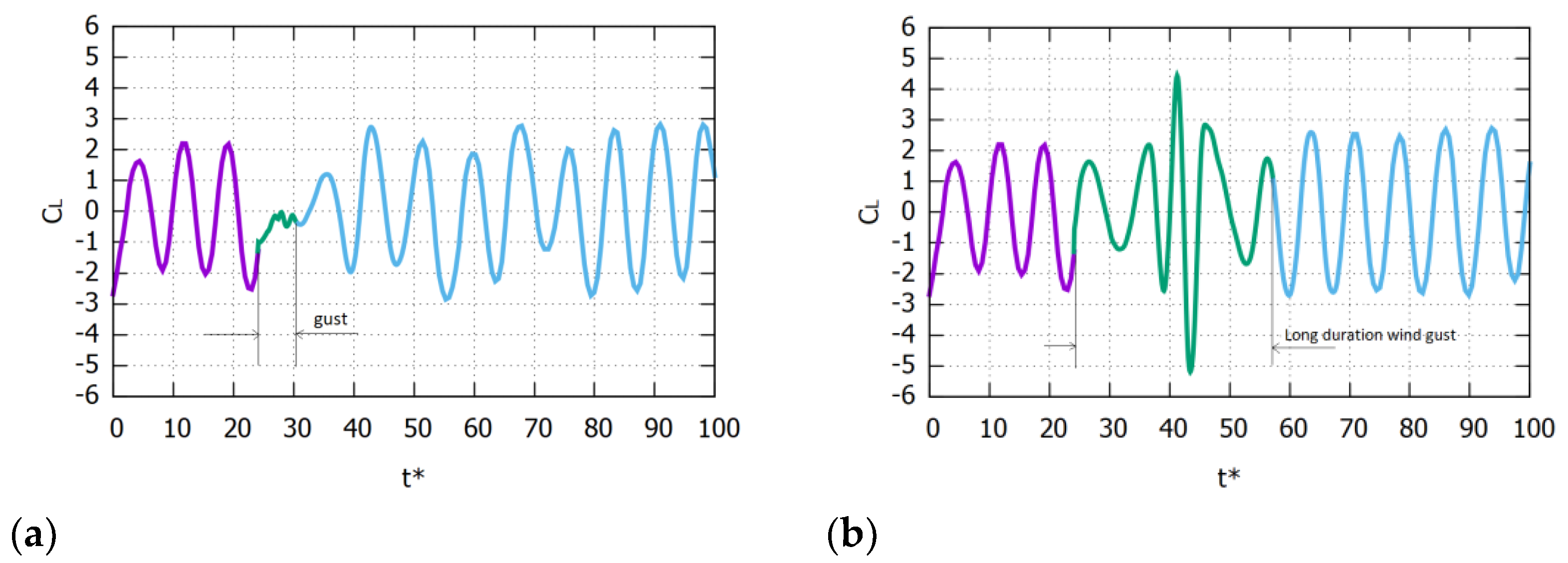
3.2. Gust Introduction in Flow Past a Square Cylinder

For implementation of the wind gusts, described in Section 2.3, the inlet velocity profile of Equation (8) and Figure 2 was applied with a period of T1 = 20 s. and T2 = 100 s for a wind gust of short and long duration, respectively. These test cases were conducted with free-stream boundary conditions on the two sides in the lateral dimension.
Points a, b, c, d, and e in Figure 2 denote particular instances of time that are denoted in the same manner in Figure 12, Figure 13 and Figure 14. In Figure 12, the contours of the streamwise velocity are presented for the steady-state upstream flow before any gust begins, at position a in Figure 2.
On the other hand, Figure 13b1,b2 correspond to time instance b, i.e., at the end of the initial reduction of velocity. Although the absolute decrease in velocity value is the same for the two gusts, the effect of their duration is already evident as, in Figure 13b1 for the short-duration gust, the absolute value of velocity is smaller in the wake than in Figure 13b2, where, due to the longer duration, the inlet velocity was reduced at a slower rate.
Figure 13c1,2 presents the flow field when the inlet velocity reaches its maximum value. For the longer gust duration (Figure 13c2), a large region of flow reversal appears in the wake of the rod, which is almost completely absent for the gust of shorter duration (Figure 13c1). Points b and d in Figure 2 correspond to the same inlet velocity, but the time history of the velocity leads to Figure 13b1,2,d1,2 having completely different flow fields.
It is impressive to note the symmetric regions that appear above and below the square cylinder for the shorter-duration gust, which persist until the gust is over (Figure 13e1). However, when the longer-duration gust is introduced, the rate of change of upstream velocity is slower, and the general form of the natural vortex-shedding sequence is still recognizable. This observation may be examined in relation to the natural vortex-shedding period, which was 23.5 s, slightly longer than the short-duration gust. On the other hand, the gust of longer duration contains more than four natural vortex-shedding periods. This behavior is reminiscent of the lock-on phenomenon, which appears when the frequency of model oscillation, or upstream velocity fluctuation frequency, approaches the natural shedding frequency [67,68].
In Figure 14, contours of streamwise velocity are presented after the end of the gust duration. The letters f, g, h, and i correspond to 25%, 50%, 75%, and 100% of each gust’s period, respectively. Therefore, Figure 14f1–i1 and Figure 14f2–i2 present results that correspond to less than one natural vortex-shedding period and more than four vortex-shedding periods of each gust, respectively. When the short-duration gust is over, the flow needs more than half of a gust period to recover, and the pair-vortex created on the sides of the rod persists until then.
On the other hand, for the longer-duration gust, the flow recovers almost immediately, and the flow field seems to continue as if the gust never happened. It should be kept in mind though that 25% of the long-duration gust period corresponds to roughly one natural shedding period and/or one short-duration gust period.
In Figure 15, the timeseries of the streamwise velocity component at the centerline, five cylinder side lengths downstream (x/D = 5), is presented. The shape of the gust signal applied at the inlet (Figure 2) is barely recognizable in either of the two curves (the gust begins at t* = 25). While the peak is obvious in both cases, the initial decrease in wind velocity, i.e., at the beginning of the gust, is bigger than the one near the end of the shorter-duration gust, while this is reversed for the longer-duration gust. As was obvious from the contours in Figure 13, velocity fluctuations were larger when the longer-duration gust was introduced. However, the delay of flow recovery is apparent in Figure 15a, after the end of the short-duration gust. Even if one considers that purely periodic behavior cannot be expected in turbulent flows, it is noteworthy that while the basic periodic behavior seems to have recovered at 60 non-dimensional time units after the long-duration gust (Figure 15b), the streamwise velocity is still not periodic at 100-non dimensional time units after the short-duration gust (Figure 15a). It should be noted that the streamwise velocity presented in Figure 15 took longer than all the other variables to recover.
The timeseries of the transverse velocity component at the same above-mentioned position (x/D = 5) is presented in Figure 16. Transverse velocity is significantly reduced, and its recovery is delayed in the case of the short-duration gust, while for the longer duration, the periodicity in the transverse velocity signal immediately recovers.
The total drag coefficient (CD) was also calculated from the difference between the pressure coefficient on the windward and leeward sides. As the friction coefficient did not have a significant contribution, CD was calculated from
c D = 2 ρ A u i n l e t 2 S P w i n d w a r d d s S P l e e w a r d d s
where ρ is air density, A is the cylinder’s frontal area, and u is the mean inlet velocity. The timeseries of total drag coefficient are presented in Figure 17 for the two gusts. For the long-duration gust, the CD time signal is similar to that of the inlet streamwise velocity.
The maximum CD value is the same in the two timeseries, but when it comes to the short-duration gust, after reaching the maximum value, its value significantly drops (the corresponding time-instance is that of point d1 in Figure 2) and eventually reaches a negative value.
The lift coefficient is calculated in a similar way to the drag coefficient through the difference in pressures exerted on the upper and lower side of the cylinder:
c L = 2 ρ A u i n l e t 2 S P u p p e r d s S P l o w e r d s
The timeseries of the lift coefficient are presented in Figure 18, and it is notable that throughout the short-duration gust, CL is almost zero. On the other hand, for the gust of longer duration, the total lift coefficient still maintains its periodicity, but there is a single fluctuation that has a value exceeding those of the previous and following periods. It is evident that the gust influence in the lateral direction is significant and also depends on the duration of the gust, i.e., the frequency of the fluctuation in relation to the natural shedding frequency.
In an effort to further analyze the behavior of the drag and lift coefficients, timeseries of the pressure coefficients on the windward and leeward sides are presented in Figure 19. These correspond to the first and second term of Equation (11), respectively. These curves are expected to be proportional to the CD curve in Figure 17, but the individual behavior and the phase lag between opposing sides holds important information that is lost in the total drag.
During the short-duration gust, the curves of the upwind and leeward pressure coefficients have a similar shape, but as expected, cp on the windward side is over twice the value of the leeward side. Interestingly, when the inlet velocity takes its maximum value (according to Figure 2), cp is significantly increased, as expected, but the subsequent steep drop in inlet velocity corresponds to an extreme drop in cp, (proportionally bigger than the drop in inlet velocity). On the contrary, when a longer-duration gust occurs, cp changes smoothly, and although, again, the second steep drop is much bigger than the first one, the values of cp are approximately half those of the short-duration gust.
The timeseries of pressure coefficients calculated on the upper and lower sides of the square cylinder are presented in Figure 20. Again, these coefficients correspond to the first and second term of Equation (12), respectively, and have mostly negative values due to the suction appearing relative to the free-stream reference pressure. During the short-duration gust, the two coefficients are almost the same, as expected from Figure 18, where the total lift coefficient was zero. Additionally, the values of the two pressure coefficients are significantly reduced when the steep drop in inlet velocity occurs after the gusts peak. However, for a longer-duration gust, CP changes smoothly on the top and bottom sides, their periodicity is recognizable throughout the gust, and, when it is over, they recover their initial values and periodicity very quickly. Furthermore, the two pressure coefficients continue to have a different phase, contrary to the short-duration gust, where the two pressure coefficients have the same phase and magnitude.
In Figure 21, Lissajous curves are also presented, with CD on the horizontal axis and CL on the vertical axis. When the short-duration gust occurs, CL is zero, and the shape of the Lissajous curve is not maintained during the gust. However, when a longer-duration gust occurs, the velocity slowly changes, and some form of periodicity is maintained even for the duration of the gust. Therefore, the Lissajous curve loop is displaced during the long duration gust, maintaining almost the same shape but returning to its initial position immediately after the gust.

4. Discussion and Conclusions

Single wind gusts of short and long duration were applied upstream of a square cylinder in order to investigate their effect on global characteristics, such as the wake, the drag and lift coefficients, and the pressure distribution on the cylinder’s outer surfaces. Although these characteristics are most often of interest to applications related to the forces acting on the bluff body, when dealing with free-standing constructions such as towers or buildings, the pressure differences are also relevant to infiltration and ventilation.
This research was carried out by implementing a very large eddy simulation (VLES) model to an in-house code, which was then successfully validated against results from the literature for a square cylinder exposed to a steady upstream flow. The validated in-house code was then used to study the effect of two upstream gusts, whose differences lie in their duration but not in the values of the mean inlet velocity or the gust amplitude. The duration of the short gust was very close to the natural vortex-shedding period, and the longer gust duration is four times larger.
The change in behavior of the flow characteristics was found to be significant under the influence of the gusts. Detailed comparison and quantitative discussions have already been presented along with the results, but the applied implications are further discussed here. For the short-duration gust, the behavior closely resembles the lock-on phenomenon frequently visited in case of a periodic upstream velocity fluctuation; i.e., the gust’s sudden change in inlet velocity breaks the alternating vortex-shedding pattern and results in the creation of pair-vortex-shedding, as the two vortices shed simultaneously from the lateral sides. On the other hand, for the longer gust duration, the gradual change in the velocity allows the flow to maintain its vortex-shedding periodicity even though the amplitude of the gust is the same as in the previous case. This conclusion agrees with the expected behavior for upstream perturbation frequencies close (short-duration gust) or far (long-duration gust) to the natural shedding frequency of the cylinder.
It is interesting to discuss the implications of the formation of the pair-vortex during the short gust duration, as it leads to simultaneously occurring, identical pressure coefficients on the lateral sides of the cylinder, and so the overall lift coefficient is close to zero. This occurs even though these pressure coefficients are more than twice as large as those for the gust of long duration. In the case of a hollow structure, such as a building, where air exchange is determined by pressure differences, short-duration gusts would induce minimal cross-ventilation air exchange in the lateral direction.
Conversely, more efficient lateral air exchange is achieved for longer-duration gusts because although the pressure coefficients are of lower magnitude, their variation is out of phase and leads to an overall pressure difference across the building. When it comes to the streamwise direction, the differences between the short- and long-duration gust do not significantly affect the maximum values of the total drag coefficients. However, for the case of the short-duration gust, the total drag coefficient and even the windward pressure coefficient obtains a negative value near the end of the gust, indicating air exfiltration even from the windward side.
An overall observation is that gust occurrence will contribute to air exchange, but depending on the duration of the gust, this may or may not be significant in the streamwise or lateral direction. For the short-duration gust, occurring close to the natural shedding period of the cylinder, streamwise air exchange is favored, notably in both upstream and downstream directions, but lateral air exchange is minimal. Longer-duration gusts may induce significant lateral air exchange and streamwise exchange in the downstream direction. It should be noted that the present study did not examine different gust periods to find the development of the behavior as gust duration increases, nor was the overall exchanged air volume considered, especially for the case of repeated gusts of the same or different duration. These are novel observations that justify further research with relevance to air infiltration and building natural ventilation.

Author Contributions

Conceptualization, D.B. and M.K.; methodology, D.B. and M.K.; software, D.B. and M.K.; validation, D.B. and M.K.; formal analysis, D.B. and MK.; investigation, D.B. and M.K.; data curation, D.B. and M.K.; writing—original draft preparation, M.K.; writing—review and editing, D.B.; visualization, D.B. and M.K. All authors have read and agreed to the published version of the manuscript.

Funding

This research received no external funding.

Data Availability Statement

Data are contained within the article.

Conflicts of Interest

The authors declare no conflict of interest.

References

  1. Boettcher, F.; Renner, C.; Waldl, H.P.; Peinke, J. On the statistics of wind gusts. Bound. Layer Meteorol. 2003, 108, 163–173. [Google Scholar] [CrossRef]
  2. Yan, B.; Chan, P.; Li, Q.; He, Y.; Cai, Y.; Shu, Z.; Chen, Y. Characterization of Wind Gusts: A Study Based on Meteorological Tower Observations. Appl. Sci. 2022, 12, 2105. [Google Scholar] [CrossRef]
  3. Wu, Z.; Cao, Y.; Ismail, M. Gust loads on aircraft. Aeronaut. J. 2019, 123, 1216–1274. [Google Scholar] [CrossRef]
  4. Granlund, K.; Monnier, B.; Ol, M.; Williams, D. Airfoil longitudinal gust response in separated vs. attached flows. Phys. Fluids 2014, 26, 027103. [Google Scholar] [CrossRef]
  5. Montenegro, P.A.; Heleno, R.; Carvalho, H.; Calcada, R.; Baker, C.J. A comparative study on the running safety of trains subjectedto crosswinds simulated with different wind models. J. Wind Eng. Ind. Aerodyn. 2020, 207, 104398. [Google Scholar] [CrossRef]
  6. Rakib, M.I.; Evans, S.P.; Clausen, P.D. Measured gust events in the urban environment, a comparison with the IEC standard. Renew. Energy 2020, 146, 1134–1142. [Google Scholar] [CrossRef]
  7. Quan, Y.; Wang, S.; Gu, M.; Kuang, J. Field measurement of wind speeds and wind-induced responses atop the shanghai worldfinancial center under normal climate conditions. Math. Probl. Eng. 2013, 2013, 902643. [Google Scholar] [CrossRef]
  8. Wu, Y.; Li, Q.; Li, G.; He, B.; Dong, L.; Lan, H.; Zhang, L.; Chen, S.; Tang, X. Vertical Wind Speed Variation in a Metropolitan City inSouth China. Earth Space Sci. 2022, 9, e2021EA002095. [Google Scholar] [CrossRef]
  9. Da Rosa, C.E.; Stefanello, M.; Facco, D.S.; Roberti, D.R.; Rossi, F.D.; Nascimento, E.L.; Degrazia, G.A. Regional-scale meteorological characteristics of the Vento Norte phenomenon observed in Southern Brazil. Environ. Fluid Mech. 2022, 22, 819–837. [Google Scholar] [CrossRef]
  10. Van de Walle, J.; Thiery, W.; Brogli, R.; Martius, O.; Zscheischler, J.; van Lipzig, N.P.M. Future intensification of precipitation and wind gust associated thunderstorms over Lake Victoria. Weather. Clim. Extrem. 2021, 34, 100391. [Google Scholar] [CrossRef]
  11. Jielan, X.; Changxing, L.; Honglong, Y.; Ruiquan, G.; Chao, L.; Baomin, W.; Pak, W.H.; Shaojia, F.; Lei, L. Tower-observed structural evolution of the low-level boundary layer before, during, and after gust front passage in a coastal area at low latitude. Weather. Clim. Extrem. 2022, 36, 100429. [Google Scholar]
  12. An, Y.; Quan, Y.; Gu, M. Field measurement of wind characteristics of Typhoon Muifa on the Shanghai world financial center. Int. J. Distrib. Sens. Netw. 2012, 8, 893739. [Google Scholar] [CrossRef]
  13. Wang, X.J.; Li, Q.S.; Yang, J.W. Non stationary near-ground wind characteristics and wind-induced pressures on the roof of a low-rise building during a typhoon. J. Build. Eng. 2022, 53, 104492. [Google Scholar] [CrossRef]
  14. Li, L.; Zhou, Y.; Wang, H.; Zhou, H.; He, X.; Wu, T. An analytical framework for the investigation of tropical cyclone wind characteristics over different measurement conditions. Appl. Sci. 2019, 9, 5385. [Google Scholar] [CrossRef]
  15. Piquee, J.; García-Risco, A.Á.; López, I.; Breitsamte, C.; Wüchner, R.; Bletzinger, K.U. Numerical investigations of a membrane morphing wind turbine blade under gust conditions. J. Wind. Eng. Ind. Aerodyn. 2022, 224, 104921. [Google Scholar] [CrossRef]
  16. Bai, H.; Aoues, Y.; Cherfils, J.M.; Lemosse, D. Design of an active damping system for vibration control of wind turbine towers. Infrastructures 2021, 6, 162. [Google Scholar] [CrossRef]
  17. Nasef, S.A.; Hassan, A.A.; Elsayed, H.T.; Zahran, M.B.; El-Shaer, M.K.; Abdelaziz, A.Y. Optimal Tuning of a New Multi-input Multi-output Fuzzy Controller for Doubly Fed Induction Generator-Based Wind Energy Conversion System. Arab. J. Sci. Eng. 2022, 47, 3001–3021. [Google Scholar] [CrossRef]
  18. Basker, I.; NainangkuppamVenkatesan, M. 3D-CFD flow driven performance analysis of new non-cylindrical helical vertical axis wind turbine for fluctuating urban wind conditions. Energy Sources Part A Recovery Util. Environ. Eff. 2022, 44, 2186–2207. [Google Scholar] [CrossRef]
  19. Iori, J. Design optimization of a wind turbine blade under non-linear transient loads using analytic gradients. J. Phys. Conf. Ser. 1618, 2020, 042032. [Google Scholar] [CrossRef]
  20. Parekh, C.J.; Roy, A.; Harichandan, A.B. Numerical simulation of incompressible gusty flow past a circular cylinder. AEJ Alex. Eng. J. 2018, 57, 3321–3332. [Google Scholar] [CrossRef]
  21. Afgan, I.; Benhamadouche, S.; Han, X.; Saugaut, P.; Laurence, D. Flow over a flat plate with uniform inlet and incident coherent gusts. J. Fluid Mech. 2013, 720, 457–485. [Google Scholar] [CrossRef] [Green Version]
  22. Golubev, V.V.; Dreyer, B.D.; Hollenshade, T.M. High-accuracy viscous analysis of unsteady flexible airfoil response to impinging gust. In Proceedings of the 15th AIAA/CEAS Aeroacoustics Conference, Miami, FL, USA, 11–13 May 2009. [Google Scholar]
  23. Bierbooms, W.; Cheng, P.W. Stochastic gust model for design calculation of wind turbine. J. Wind Eng. Ind. Aerodyn. 2002, 90, 1237–1251. [Google Scholar] [CrossRef]
  24. Bierbooms, W. A gust model for wind turbine design. JSME Int. J. Ser. B. 2004, 47, 378–386. [Google Scholar] [CrossRef]
  25. Available online: https://graphical.weather.gov/ (accessed on 13 August 2013).
  26. Kasperski, M. A consistent model for the codification of wind loads. J. Wind Eng. Ind. Aerodyn. 2007, 95, 1114–1124. [Google Scholar] [CrossRef]
  27. TC88 WG1. IEC 61400-1; Wind Turbines: Design Requirements. International Electrotechnical Commission: London, UK, 2005.
  28. Shirzadeh, K.; Hangan, H.; Crawford, C. Experimental and numerical simulation of extreme operational conditions for horizontal axis wind turbines based on the IEC standard. Wind. Energy Sci. 2020, 5, 1755–1770. [Google Scholar] [CrossRef]
  29. Huang, R.F.; Hsu, C.M.; Chiu, P.C. Flow behavior around a square cylinder subject to modulation of a planar jet issued from upstream surface. J. Fluids Struct. 2014, 51, 362–383. [Google Scholar] [CrossRef]
  30. Xiaoqing, D.; Ruyi, C.; Hanlin, X.; Wenyong, M. Experimental study on aerodynamic characteristics of two tandem square cylinders. Fluid Dyn. Res. 2019, 51, 055508. [Google Scholar] [CrossRef]
  31. Williamson, C. Vortex dynamics in the cylinder wake. Annu. Rev. Fluid Mech. 1996, 28, 477–539. [Google Scholar] [CrossRef]
  32. Zhang, D.; Cheng, L.; An, H.; Zhao, M. Direct numerical simulation of flow around a surface-mounted finite square cylinder at low Reynolds numbers. Phys. Fluids 2017, 29, 045101. [Google Scholar] [CrossRef]
  33. Wang, Y.Q. Effects of Reynolds number on vortex structure behind a surface-mounted finite square cylinder with AR = 7. Phys. Fluids 2019, 31, 115103. [Google Scholar] [CrossRef]
  34. Sohankar, A.; Norberg, C.; Davidson, L. Simulation of three-dimensional flow around a square cylinder at moderate Reynolds numbers. Phys. Fluids 1999, 11, 288. [Google Scholar] [CrossRef]
  35. Akamura, Y.N. Vortex shedding from bluff bodies and a universal Strouhal number. J. Fluids Struct. 1996, 10, 159–171. [Google Scholar] [CrossRef]
  36. Meng, H.; Chen, W.; Chen, G.; Gao, D.; Li, H. Characteristics of forced flow past a square cylinder with steady suction at leading-edge corners. Phys. Fluids 2022, 34, 025119. [Google Scholar] [CrossRef]
  37. Etheridge, D.W.; Sandberg, M. Building Ventilation: Theory and Measurement; John Wiley & Sons: Chichester, UK, 1996. [Google Scholar]
  38. Finnegan, M.; Pickering, C.A.; Burge, P.S. The sick building syndrome: Prevalence studies. Med.Br. J. 1984, 289, 1573–1575. [Google Scholar] [CrossRef] [PubMed]
  39. Tominaga, Y.; Blocken, B. Wind tunnel analysis of flow and dispersion in cross-ventilated isolated buildings: Impact of opening positions. J. Wind Eng. Ind. Aerod. 2016, 155, 74–88. [Google Scholar] [CrossRef]
  40. Tong, Z.; Chen, Y.; Malkawi, A. Defining the Influence Region in neighborhood scale CFD simulations for natural ventilation design. Appl. Energy 2016, 182, 625–633. [Google Scholar] [CrossRef]
  41. Hooff, T.; Blocken, B.; Tominaga, Y. On the accuracy of CFD simulations of cross-ventilation flows for a generic isolated building: Comparison of RANS, LES and experiments. Build. Environ. 2017, 114, 148–165. [Google Scholar] [CrossRef]
  42. Norberg, C. Flow around rectangular cylinders: Pressure forces and wake frequencies. J. Wind Eng. Ind. Aerodyn. 1993, 49, 187–196. [Google Scholar] [CrossRef]
  43. Luo, S.C.; Yazdani, M.G.; Chew, Y.T.; Lee, T.S. Effects of incidence and after body shape on flow past bluff cylinders. J. Wind Eng. Ind. Aerodyn. 1994, 53, 375–399. [Google Scholar] [CrossRef]
  44. Lyn, D.; Rodi, W. The flapping shear layer formed by flow separation from the forward corner of a square cylinder. J. Fluid Mech. 1994, 267, 353–376. [Google Scholar] [CrossRef]
  45. Lyn, D.A.; Einav, S.; Rodi, W.; Park, J.H. A laser-Doppler velocimetry study of ensemble-averaged characteristics of the turbulent near wake of a square cylinder. J. Fluid Mech. 1995, 304, 285–319. [Google Scholar] [CrossRef]
  46. Minguez, M.; Brun, C.; Pasquetti, R.; Serre, E. Experimental and high-order LES analysis of the flow in near-wall region of a square cylinder. Int. J. Heat Fluid Flow 2011, 32, 558–566. [Google Scholar] [CrossRef]
  47. Sohankar, A.; Davidson, L. Large eddy simulation of flow past a square cylinder: Comparison of different subgrid scale models. ASME J. Fluids Eng. 2000, 122, 39–47. [Google Scholar] [CrossRef]
  48. Rodi, W.; Ferziger, J.H.; Breuer, M.; Pourquié, M. Status of large eddy simulation: Results of a workshop. J Fluids Eng. Trans. ASME 1997, 119, 248–262. [Google Scholar] [CrossRef]
  49. Rodi, W. Comparison of LES and RANS calculations of the flow around bluff bodies. J. Wind Eng. Ind.Aerodyn. 1997, 6971, 55–75. [Google Scholar] [CrossRef]
  50. Trias, F.X.; Gorobetsab, A.; Olivaa, A. Turbulent flow around a square cylinder at Reynolds number 22,000: A DNS study. Comput. Fluids 2015, 123, 87–98. [Google Scholar] [CrossRef]
  51. Verstappen, R.W.C.P.; Veldman, A.E.P. Spectro-consistent discretization of Navier–Stokes: A challenge to RANS and LES. J. Eng. Math. 1998, 34, 163–179. [Google Scholar] [CrossRef]
  52. Barone, M.F.; Roy, C.J. Evaluation of detached eddy simulation for turbulent wake applications. AIAA J. 2006, 44, 3062–3071. [Google Scholar] [CrossRef]
  53. Speziale, C.G. Turbulence modeling for time-dependent RANS and VLES: A review. AIAA J. 1998, 36, 173–184. [Google Scholar] [CrossRef]
  54. Girimaji, S.S.; Srinivasan, R.; Jeong, E. PANS turbulence for seamless transition between RANS andLES: Fixed-point analysis and preliminary results. In Proceedings of the ASME/JSME 2003 4th Joint Fluids Summer Engineering Conference, Honolulu, HI, USA, 6–10 July 2003. [Google Scholar]
  55. Han, X.; Krajnovic, S. An efficient very large eddy simulation model for simulation of turbulent flow. Int. J. Numer. Meth. 2012, 71, 1341–1360. [Google Scholar] [CrossRef]
  56. Patankar, S.V.; Spalding, D.B. A calculation procedure for heat, mass and momentum transfer in three-dimensional parabolic flows. Int. J. Heat Mass Transf. 1972, 15, 1787–1806. [Google Scholar] [CrossRef]
  57. Papadakis, G.; Bergeles, G. A locally modified 2nd-order upwind scheme for convection terms discretization. Int. J. Fluids Struct. 1995, 9, 435–455. [Google Scholar]
  58. Barmpas, F.; Bouris, D.; Moussiopoulos, N. 3D Numerical Simulation of the Transient Thermal Behavior of a Simplified BuildingEnvelope Under External Flow. J. Sol. Energy Eng. 2009, 131, 031001. [Google Scholar] [CrossRef]
  59. Jurelionis, A.; Bouris, D.G. Impact of Urban Morphology on Infiltration-Induced Building Energy Consumption. Energies 2016, 9, 177. [Google Scholar] [CrossRef]
  60. Bouris, D.; Triantafyllou, A.G.; Krestou, A.; Leivaditou, E.; Skordas, J.; Konstantinidis, E.; Kopanidis, A.; Wang, Q. Urban-Scale Computational Fluid Dynamics Simulations with Boundary Conditions from Similarity Theory and a Mesoscale Model. Energies 2021, 14, 5624. [Google Scholar] [CrossRef]
  61. Stull, R. Practical Meteorology: An Algebra-Based Survey of Atmospheric Science; Dept. of Earth, Ocean & Atmospheric Sciences, University of British Columbia: Vancouver, BC, Canada, 2015. [Google Scholar]
  62. Letson, F.; Barthelmie, R.J.; Hu, W.; Pryor, S.C. Characterizing wind gusts in complex terrain. Atmos. Chem. Phys. 2019, 19, 3797–3819. [Google Scholar] [CrossRef]
  63. Wind tunnel studies of buildings and structures. In ASCE Manuals and Reports on Engineering Practice; No. 67; Isyumov, N. (Ed.) Aerospace Division of the American Society of Civil Engineers: Reston, VI, USA, 1999. [Google Scholar]
  64. Franke, R.; Rodi, W. Calculation of vortex shedding past a square cylinder with various turbulence models. In Turbulent Shear Flows 8; Springer: Berlin/Heidelberg, Germany, 1991. [Google Scholar]
  65. Bouris, D.; Bergeles, G. 2D LES of vortex shedding from a square cylinder. J. Wind Eng. Ind. Aerodyn. 1999, 80, 31–46. [Google Scholar] [CrossRef]
  66. Raisee, M.; Jafari, A. Numerical Study of Turbulent Flow around a Square Cylinder Using Two Low-Reynolds-Number K − ε Models. In European Conference on Computational Fluid Dynamics; Wesseling, P., Oñate, E., Périaux, J., Eds.; TU Delft: Delft, The Netherlands, 2006. [Google Scholar]
  67. Barbi, C.; Favier, D.; Maresca, C.; Telionis, D. Vortex shedding and lock-on of a circular cylinder in oscillatory flow. J. Fluid Mech. 1986, 170, 527–544. [Google Scholar] [CrossRef]
  68. Konstantinidis, E.; Bouri, D. Vortex synchronization in the cylinder wake due to harmonic and non-harmonic perturbations. J. Fluid Mech. 2016, 804, 248–277. [Google Scholar] [CrossRef]
Figure 1. (a) Schematic of the modeling domain; (b) computational grid.
Fluids 07 00303 g001
Figure 2. Inlet gust velocity signals for two different gust durations.
Fluids 07 00303 g002
Figure 3. Calculated streamwise velocity timeseries at x/D = 5.
Fluids 07 00303 g003
Figure 4. Mean y+ values along the square cylinder sides for steady upstream velocity.
Fluids 07 00303 g004
Figure 5. Ratio of effective to laminar viscosity (μ + μt)/μ in the vicinity of the square rod.
Fluids 07 00303 g005
Figure 6. Comparison of mean streamwise velocity along the central line including results from Sohankaret al.’s LES [47], Hanet al.’s VLES [55], Lyn’s experiment [45], and Franke and Rodi’s [64] k-ε results.
Fluids 07 00303 g006
Figure 7. Comparison of the RMS velocity profiles along the central line (see sketch above graphs), including results from Sohankar et al.’s LES [47], Han et al.’s VLES [55], and Lyn et al.’s experiment [45]: (a) uRMS velocity, (b) uRMS velocity, (c) wRMS velocity.
Fluids 07 00303 g007
Figure 8. Comparison of total fluctuation energy along the central line, including Bouris and Bergeles’s 2D-LES [65] results and Lyn et al.’s experiment [45].
Fluids 07 00303 g008
Figure 9. Comparison of (a) mean streamwise and (b) transverse velocity profiles at x/D = 1 (see sketch above graphs), including Han and Kranjovic’s VLES [55] results and Lyn et al.’s experimental [45] results.
Fluids 07 00303 g009
Figure 10. Streamlines of the average flow.
Fluids 07 00303 g010
Figure 11. Streamlines of one period at six different time steps.
Fluids 07 00303 g011
Figure 12. Contours of the streamwise velocity before gust begins (point a in Figure 2).
Fluids 07 00303 g012
Figure 13. Streamwise velocity contours at time instants (bι), (cι), (dι), and (eι) of Figure 2. Index ι = 1 is for the short-duration (20 s) gust and ι = 2 for the long-duration (100 s) gust.
Fluids 07 00303 g013
Figure 14. Contours of the streamwise velocity after the end of a short- and long-duration gust, index ι = 1 and ι = 2, respectively, where (fι), (gι), (hι), and (iι) correspond to 25%, 50%, 75%, and 100% of each gust’s period, respectively.
Fluids 07 00303 g014
Figure 15. Timeseries of the streamwise velocity at x/D = 5 for short (a) and long gust duration (b).
Fluids 07 00303 g015
Figure 16. Timeseries of the transverse velocity at x/D = 5 for gust of short (a) and long duration (b).
Fluids 07 00303 g016
Figure 17. Timeseries of total drag coefficients for gust of (a) short and (b) long duration.
Fluids 07 00303 g017
Figure 18. The timeseries of total lift coefficients for short (a) and long (b) gust duration.
Fluids 07 00303 g018
Figure 19. Timeseries of cp on windward and leeward rod sides for gust of short (a) and long duration (b).
Fluids 07 00303 g019
Figure 20. Timeseries of CP on upper and lower rod sides for gust of short (a) and long (b) duration.
Fluids 07 00303 g020
Figure 21. Lissajous curves for gust of short (a) and long (b) duration.
Fluids 07 00303 g021
Table 1. Comparison of the global flow parameters including results from Sohankar et al.’s LES [47], Han et al.’s VLES [55], Lyn et al.’s experiment [45], and Baroneet al.’s DES [52].
Re<CD>CDrmsCLrms
Present VLES-M378 (No-slip wall)22,0002.280.221.62
Present VLES-M378 (Free-slip wall)22,0002.250.271.61
Present VLES-M575 (No-slip wall)22,0002.330.221.64
VLES -M1 [55]22,0002.210.181.36
VLES -M2 [55]22,0002.280.191.51
LES [47]22,0002.03–2.320.16–0.201.23–1.54
DES [52]19,4002.110.261.16
Experiment [45]21,4002.10--
Publisher’s Note: MDPI stays neutral with regard to jurisdictional claims in published maps and institutional affiliations.

