Article

CHP-Based Economic Emission Dispatch of Microgrid Using Harris Hawks Optimization

1
Department of Electrical Engineering, MITS, Gwalior 474005, India
2
Department of Electrical Engineering, BIT, Sindri 828123, India
3
Department of Railroad and Electrical Engineering, Woosong University, Daejeon 34606, Korea
*
Author to whom correspondence should be addressed.
Fluids 2022, 7(7), 248; https://doi.org/10.3390/fluids7070248
Submission received: 28 June 2022 / Revised: 8 July 2022 / Accepted: 13 July 2022 / Published: 18 July 2022
(This article belongs to the Special Issue Wind and Wave Renewable Energy Systems, Volume II)

Abstract

:
In this paper, the economically self-sufficient microgrid is planned to provide electric power and heat demand. The combined heat and power-based microgrid needs strategic placement of distributed generators concerning optimal size, location, and type. As fossil fuel cost and emission depend mainly on the types of distributed generator units used in the microgrid, economic emission dispatch is performed for an hour with a static load demand and multiple load demands over 24 h of a day. The TOPSIS ranking approach is used as a tool to obtain the best compromise solution. Harris Hawks Optimization (HHO) is used to solve the problem. For validation, the obtained results in terms of cost, emission, and heat are compared with the reported results by DE and PSO, which shows the superiority of HHO over them. The impact of renewable integration in terms of cost and emission is also investigated. With renewable energy integration, fuel cost is reduced by 18% and emission is reduced by 3.4% for analysis under static load demand, whereas for the multiple load demands over 24 h, fuel cost is reduced by 14.95% and emission is reduced by 5.58%.

1. Introduction

In the past decades, the attention toward microgrid (MG) operation has increased with the integration of distributed generation (DG) units near the consumer end to fulfill the power demand. The MG has been characterized as a small-scale, self-sustaining cluster distribution power system architecture that combines multiple DG, combined heat and power (CHP) units, energy storage systems (ESSs), and load, acting as a single and controllable entity [1]. Integrating CHP units in the MG has attracted more attention with the motivation to provide thermal energy with electric power by using the waste heat generated during electricity generation [2]. The successful implementation of bio-inspired evolutionary optimization techniques in solving many complex engineering problems has attracted researchers to apply different optimization algorithms to solve the load dispatch problems using several test cases of power systems.
The combined heat and power dispatch (CHPED) problem has been realized using a real coded genetic algorithm [3], improved group search algorithm [4], oppositional teaching-learning based optimization [5], modified particle swarm optimization (PSO) [6], self-regulating PSO [7], cuckoo search algorithm (CSA) [8], gravitational search algorithm [9], exchange market algorithm [10], group search algorithm [11], and grey wolf optimization (GWO) [12] using different test cases. The demand-side management and the optimal operational problem of the MG were studied using a hybrid genetic algorithm (GA) and artificial bee colony (ABC) algorithm. Here, the objective is to minimize overall running costs of the MG, demand-side management costs, and costs due to load shifting [13]. A hybrid artificial neural network (ANN) and PSO model were used to solve the biomass gasification plant (BGP) problem. This model was used to estimate the amount of biomass that was used to produce the required syngas, which is needed to meet the energy demand [14]. To enhance power exchange, the two-round fuzzy-based speed (TRFS) algorithm followed Stackelberg’s game theory, and the Quasi-oppositional Symbiotic Organism Search Algorithm was used in a multi-MG environment to study the power exchange problem [15].
The power generating units using fossil fuels emit pollutant gases in the environment. These environmental concerns have pushed toward the integration of DGs based on clean and renewable resources. At the same time, emission constraints have also been considered in the scheduling problem. The economic dispatch and emission dispatch are single objectives to minimize the fuel cost and emission, respectively, by determining the optimal generation of each unit in the system while satisfying the demand load and other operational constraints. However, the results showed conflict with each other, i.e., minimizing fuel costs increases the emissions and vice-versa. Therefore, a multiobjective approach has been used to deal with these two conflicting objectives in the combined CHP economic and emission dispatch (CHPEED) problem. The CHPEED multi-objective problem has been solved using numerical polynomial homotopy continuation (NPHC) [16], the normal boundary intersection method [17], time-varying acceleration PSO [18], GWO [19], and multiverse optimization [20].
Integrating renewable-based DG such as wind and solar power with conventional units reduced environmental emissions. In Ref. [21], a comparative analysis was conducted to solve the power dispatch problem using different BI optimization methods for various test systems with the integration of wind units. The wind and fuel cell unit were integrated with the thermal plant to analyze economic dispatch and the MG power dispatch problem using CSA [22]. The solar and wind unit was incorporated with the thermal plant to investigate the CHPED using the squirrel search algorithm [23]. The impact on cost and emission with the integration of renewable-based DG was analyzed using an equilibrium optimizer (EO) [24]. The EED problem in a wind power integrated system was analyzed to estimate the impact of carbon trading prices on the reduction in carbon emission and enhancing the efficiency of power generation efficiency improvements [25]. To achieve the desired scenario of zero greenhouse gas emissions, the techno-economic feasibility analysis was carried out under different scenarios of the combined usage of renewable-based DG and storage systems [26]. The scheduling problem of MG having DG and wind units under their respective limits was performed using the manta ray foraging algorithm (MRFO). The effect on the cost due to the integration of solar power and energy storage systems was also examined [27]. The MG was reconfigured to analyze the demand response program using PSO to reduce the conventional DGs’ fuel cost and the cost of acquiring electricity from the grid. The point estimate method was used to simulate the uncertainty of RESs, while the uncertainty due to other parameters was ignored [28]. A multiobjective thermal unit-based economic dispatch was carried out using binary and continuous PSO algorithms in Ref. [29]. To study the performance of MG under six distinct scenarios, the modified binary PSO was used to solve the load dispatch problem. The uncertainty of RESs, demand, and the market price was considered to neglect the system’s power loss and spinning reserve [30]. The uncertainty associated with wind power plants due to uncertain wind velocity can be modeled using penalty and reserve cost to represent their under- and overestimation of wind power, respectively [31]. In Ref. [32], DE and PSO were used to analyze the planning problem in CHP-based MG. Here, the loss-sensitive approach was used to select the bus on a 14-bus MG and to determine the optimal size of DGs using PSO for minimum loss in the system, and CHPEED was further carried out using DE and PSO.
Wolpert and Macready, in the year 1997, proposed a No free lunch theorem, which states that no single algorithm can guarantee to solve all types of optimization problems [33]. Harris Hawks Optimization (HHO) is a swarm intelligence-based optimization approach; its analytical mode takes care of distinct foraging strategies such as tracing, sieging, and surprise attacks during the optimization process [34]. HHO has been successfully applied for various real-world problems such as in cost management and the operation of multi-source-based microgrids [35], and in relay coordination problems [36]. In this paper, HHO was implemented for the solution of DG placement planning and optimum generation scheduling of a CHP-based MG.
The main contribution is as follows:
  • The HHO algorithm was implemented to analyze its effectiveness in solving the DG placement and the load dispatch problem for an MG.
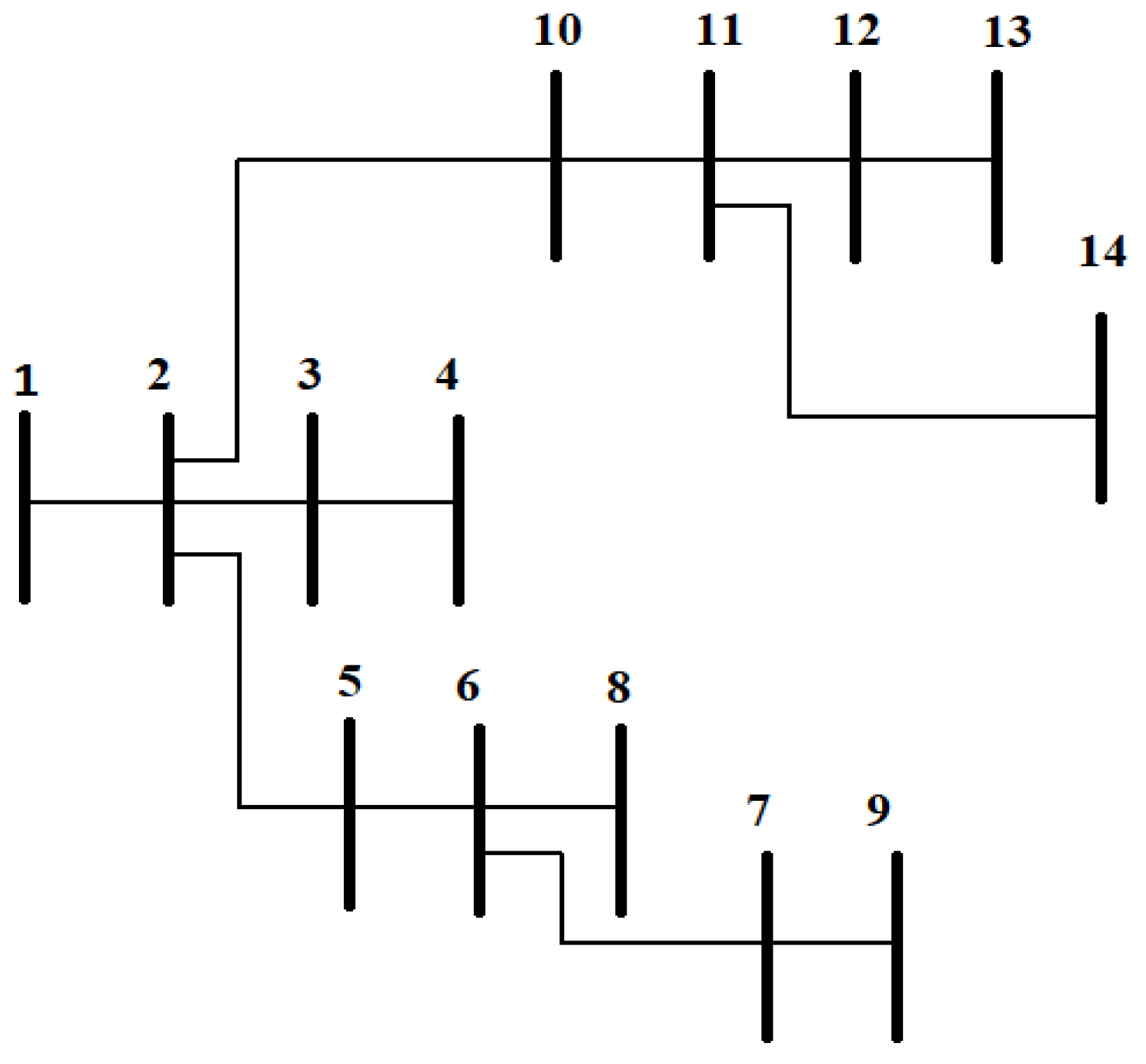
  • Selection of optimal size and location of DGs for a 14-bus RDS.
  • Load dispatch was conducted under two different scenarios (i.e., with and without renewable energy for minimization of cost and minimization of emission.
  • TOPSIS was implemented to obtain the best-compromised solution (BCS).
This paper is organized as follows: Section 2 contains the problem formulation that combines the modeling of different types of DG units, the formulation of the CHPEED problem, and operational constraints. The concept behind the HHO algorithm is presented in Section 3. Section 4 deals with the description of test cases, simulation results, and discussion. Finally, concluding remarks are discussed in Section 5.

2. Problem Formulation

This paper focuses on CHPEED-based optimal generation scheduling for effective energy management planning in MG. Here, the objective is to minimize the cost and emission due to on-site generation and the CHP system. Therefore, optimal siting and sizing of DG units are essential in this context. Its formulations are added with the CHPEED problem as below.

2.1. Optimal Placement of DG

The DG unit was placed in MG to minimize the power loss as [32]:
M i n i m u m     ( P l ) = i = 1 N g P i P d
where P l is the power loss in the system, P d is the power demand, P i is the power output of ith DG unit, and N g is the number of DG units in MG.
It is subject to the following constraints [32]:
V m i n     | V i |     V m a x
where V i   is the voltage at the ith bus, with minimum voltage V m i n = 0.95 p.u. and maximum voltage V m a x = 1.05 p.u.
P i m i n P i P i m a x
where P i m i n and P i m a x are the minimum and maximum power output of the ith DG unit, respectively.

2.2. Economic Dispatch

The total operational cost of all committed DGs units expressed as [22]
f 1 = F D G T + F W P P T + F F C T
where   f 1 is the cost function; F D G T ,   F W P P T ,     and   F F C T are the costs of conventional thermal generators, wind power plant (WPP), and fuel cell (FC) units over a period of time T, respectively [22,27].

2.2.1. Modeling of Conventional Thermal Generators

The fuel cost of conventional thermal generators is expressed as [32]
F D G T = t = 1 T i = 1 N g ( a i · ( P i t ) 2 + b i · P i t + c i )
where   a i ,   b i , and c i are the fuel cost coefficient of the ith DG unit. P i t   is the power output of the ith DG unit at the tth interval of time and N g is the number of DG units [32].

2.2.2. Modeling of Wind Power Plant

As the power generation of a wind power plant (WPP) is governed by uncertain wind velocity, its variable output characteristics are used to compute the cost of wind power. The cost of wind power generation includes the cost due to the uncertainty in it, expressed as [21,22,32].
F W P P T = t = 1 T j = 1 N w C j t ( P w j t )
where N w is the number of WPP units and
C j t ( P w j t ) = β w j P w j t + k p ( P w j ,   a v t P w j t ) + k r ( P w j t P w j ,   a v t )
where P w j t and P w j ,   a v t are the scheduled output and available wind power of the jth unit at the tth interval of time, respectively; β w j are the maintenance and operating cost in USD/kW; k p and k r are the penalty cost (underestimation) coefficient and reserve cost (overestimation) of the wind power plant, respectively [21,31]. These penalty costs and reserve costs of the wind power plant are, respectively, represented as [21,31]:
k p ( P w j ,   a v t P w j t ) = k p P w j t P w r ( P w t P w j t ) f w ( P w ) d P w
k r ( P w j t P w j ,   a v t ) = k r 0 P w j t ( P w j t P w t ) f w ( P w ) d P w
where P w r is the rated output of wind power and P w t is the output power of a wind power plant at the tth time interval, determined as [21,31]:
P w t = { P w r × ( v t v c i n ) ( v r v c i n ) kW ,           ;                             v c i n   v t   v r P w r kW ,                                   ;                               v r   v t   v c o 0 ,                                               ;             v t     v c i n     a n d   v t > v c o
where v t is the wind velocity at the tth time in m/s; v c i n , ,   v c o ,   and   v r are the cut-in velocity, cut-out velocity, and rated velocity in m/s, respectively.
To determine the penalty and reserve costs, it is necessary to select the probability distribution function ( p d f ) for wind power output. The uncertainty and irregular nature of wind speed closely follow the Weibull distribution and p d f given as [21,31]:
p d f   ( v ,   k ,   c ) = k c ( v c ) k 1 e x p ( ( v c ) k )
where k and c are p d f parameters referred to as the shape factor and scale factor, respectively. The corresponding cumulative distribution function ( c d f ) is given as [21,31]
c d f   ( v ,   k ,   c ) = 1 e x p ( ( v c ) k )
The probability of wind power is calculated as [21,31]
f w ( P w ) { P w t = P w r × ( v t     v c i n ) ( v r     v c i n ) } = p d f ( P w ) = k l v c i n c ( ( 1 + ρ l ) v c i n c ) k 1 e x p ( ( ( 1 + ρ l ) v c i n c ) k )
where
ρ = P w P w r ,   and   l = ( v r v c i n ) v c i n
f w ( P w ) { P w t = P w r } = c d f ( v c o ) + ( 1 c d f ( v r ) ) = e x p ( ( v r c ) k ) e x p ( ( v c o c ) k )
f w ( P w ) { P w t = 0 } = c d f ( v c i n ) + ( 1 c d f ( v c o ) ) = 1 e x p ( ( v c i n c ) k ) + e x p ( ( v c o c ) k )

2.2.3. Modeling of Fuel-Cell Unit

The cost of an FC unit includes the cost of fuel and the efficiency of the fuel to generate electricity expressed as [22]:
F F C T = t = 1 T ( β n a t u r a l i = 1 N F C P F C ,   i t η F C ,   i )
where β n a t u r a l is the operation and maintenance cost of FC in USD/kW; η F C ,   i and P F C ,   i t are the efficiency and output power at the tth time of the ith FC unit, respectively [22].

2.3. Emission Dispatch

The emission released due to the burning of fossil fuel in the thermal power plants is expressed as follows [21,32]:
f 2 = i = 1 N g E i t ( P i t ) = i = 1 N g ( α i · ( P i t ) 2 + β i · P i t + γ i )
where f 2 is total emission output; α i ,   β i , and γ i are the emission cost coefficient of the ith DG unit [31].

2.4. Formulation of Multiobjective CHPEED Problem

The multiobjective cost function of the CHPEED problem is given as [32]:
m i n i m i z e   ( F ) = w f 1 + ( 1 w ) f 2 P f n
where F is the total cost, P f n is the price penalty factor, w is the weighting factor, and the P f n is the ratio of fuel to the emission cost and is evaluated as:
P f n i = ( a i · ( P i m a x ) 2 + b i · P i m a x + c i ) ( α i · ( P i m a x ) 2 + β i · P i m a x + γ i )
Equation (19) is minimized and subjected to operational constraints as follows [22,32].

2.5. Constraints

Total Power generation must be equal to sum of power demand and transmission loss. It is expressed as:
i = 1 N g P i t = P d t + P l t  
where P l t is the power loss and P d t is the power demand at the tth interval of time. P l is evaluated as (22) [32]:
P l t = i = 1 N g j = 1 N g P i t · B i j · P j t + i = 1 N g B 0 i · P i t + B 00
where B i j ,   B 0 i , and B 00 are the loss coefficients.
Power generated by individual generator must vary within their minimum and maximum operating limit. It is expressed as:
P i m i n     P i t     P i m a x
P w , j m i n     P w , j t     P w , j m a x
P F C , i m i n   P F C ,   i t     P F C , i m a x
where P F C , i m i n and P w , j m i n are the minimum power output of FC and WPP units, respectively; P w , j m a x and P F C , i m a x are the maximum power output of WPP and FC units, respectively.
The change in power generating unit between two consecutive times is limited by up and down ramp limits, respectively, as follows [32]:
P i t P i t 1   U R i
P i t 1 P i t   D R i
where U R i and D R i are up and down ramp limits of the ith generating units, respectively [32].
H R = i = 1 N g θ i · P i t
where H R is the total heat output and θ i is the heat-to-power ratio of the ith DG unit [32].
i = 1 N g θ i · P i t     H D
where H D is the total heat demand.

2.6. TOPSIS

The technique of order preferences by the simulation to ideal solution (TOPSIS), initially proposed by Hwang and Yoon in 1981 [37], is a method to determine the optimal solution having the closest distance from the positive ideal solution and farthest distance from the negative ideal solution. The steps of the TOPSIS method are as follows:
Step I: Construct a decision matrix R as:
R = [ x i j ] ,         i = 1 ,   ,   m ; j = 1 , ,   n .
where x i j is the value of the jth attribute of the ith alternative.
Step II: Normalize the decision matrix R as:
r i j = x i j j = 1 m x i j 2 ,         i = 1 ,   ,   m ; j = 1 , ,   n .
Step III: Determine the weighted decision matrix as follows:
v i j = w j × r i j ,         i = 1 ,   ,   m ; j = 1 , ,   n .  
Step IV: Determine the positive and negative ideal solution computed as follows:
A + = { v 1 + ,   v 2 + ,   v 3 + , , v n + }
where
v j + = { ( max ( v i j ) ,   i f   j   J 1 ) and ( min ( v i j ) ,   i f   j   J 2 ) }
A = { v 1 ,   v 2 ,   v 3 , , v n }
where
v j = { ( min ( v i j ) ,   i f   j   J 1 ) and ( max ( v i j ) ,   i f   j   J 2 ) }
Step V: Determine the separation distance of each alternative from positive and negative ideal solutions computed as follows:
D i + = j = 1 n ( v j + v i j ) 2 ,         i = 1 ,   ,   m ; j = 1 , ,   n
D i = j = 1 n ( v j v i j ) 2 ,         i = 1 ,   ,   m ; j = 1 , ,   n
Step VI: Compute the relative closeness ( R C ) of each alternative as:
R C i = D i D i + D i + ,         i = 1 ,   ,   m ;
An R C close to one indicates the superiority of the alternative.

3. Harris Hawks Optimization

Harris Hawks Optimization (HHO) is a population-based algorithm inspired by the foraging behavior of Harris Hawks, proposed by Heidari et al. in 2019 [34]. The analytical model of HHO simulates different foraging strategies such as tracing, sieging, and surprise attacks to capture prey during optimization. The cooperative foraging behavior of Harris Hawks is as follows:
  • A prey for the Harris hawk is a rabbit having great escaping energy; therefore, several hawks cooperatively attack to prey simultaneously from different directions.
  • This attack can be completed quickly, but sometimes considering the escape ability and behavior of the prey, it takes a few short-length, quick dives nearby the prey.
  • The different phase of chasing a prey depends on the prey’s escaping pattern with other dynamic conditions.
  • The switching strategy occurs when the best hawk (leader) stops and becomes lost on the hunt, and one of the other group members will pursue the chase.
  • The Harris hawk can switch between these phases to confuse the prey, which leads to their exhaustion, and increases its vulnerability.
  • Furthermore, by confusing the escaping prey, it cannot recover its defensive abilities and, in the end, it cannot escape from the team and encounter one of the hawks, which is often the most powerful and experienced, easily grabs the tired prey, and shares it with another group member.
Different phases of HHO are shown in Figure 1 [34].

3.1. Exploration Stage

The hawks perch randomly to wait, observe, and monitor at some location to find prey based on two strategies. These strategies are mathematically modeled as:
X ( t + 1 ) = { X r a n d ( t ) r 1 | X r a n d ( t ) 2 r 2 X ( t ) | ,                           q 0.5 X r a b b i t ( t ) X m ( t ) r 3 ( L B + r 4 ( U B L B ) ) ,     q < 0.5
where X ( t + 1 ) is the position in the (t + 1)th iteration; X r a b b i t is the position of the rabbit (prey); q ,   r 1 ,   r 2 ,   r 3 ,   and r 4 are random numbers in the interval [0, 1]. U B and L B are the upper and lower bounds, respectively. X m ( t ) is the mean position of the population evaluated as:
X m = 1 N i = 1 N X i ( t )
where N is the population size, and X i ( t ) is the position of the ith individual in the tth iteration.

3.2. Transition from Exploration to Exploitation

In HHO, the rabbit’s escaping energy ‘ E ’ is used to transit between exploration and exploitation. The ‘ E ’ decreases with an increase in the iterations and is evaluated as:
E = 2 E 0 ( 1   t T )
where E 0 is the initial rabbit’s escaping energy lying in the interval [−1, 1]; t and T represent the current and maximum number of iterations, respectively. As the iteration increases, E decreases from [−2, 2] to 0. The exploration stage is used for | E | 1 , and for | E | < 1 , the exploitation is carried out to search the prey.

3.3. Exploitation Stage

In the exploitation phase, four different strategies were adopted, and they were switched between by using escape energy ‘E’; a random number r lies in the interval [0, 1], representing successful prey escape. If r < 0.5, the prey escapes successfully, while r > 0.5 means the unsuccessful escape of the prey.

3.3.1. Soft Besiege

For soft besiege, | E | 0.5 and r 0.5 represent that the prey has enough energy to escape by jumping. Hence, hawks will hunt via a soft besiege strategy modeled as:
X ( t + 1 ) = Δ X ( t ) E | J X r a b b i t ( t ) X ( t ) |  
where Δ X ( t ) represents the differences between the position of rabbits and current individuals, as given in (45). J represents the strength of the rabbit for randomly jumping during the escape and is evaluated with the random number r 5 as:
J = 2 ( 1 r 5 )  
Δ X ( t ) = X r a b b i t ( t ) X ( t )

3.3.2. Hard Besiege

For hard besiege, | E | < 0.5 and r 0.5 represent that the prey’s energy has exhausted, and hawks will hunt via a hard besiege strategy modeled as:
X ( t + 1 ) = X r a b b i t ( t ) E | Δ X ( t ) |

3.3.3. Soft Besiege with Progressive Rapid Dives

For soft besiege with progressive rapid dives, | E | 0.5 and r < 0.5 represent that the prey has enough energy. Hence, hawks will hunt via soft besiege with the progressive rapid dives strategy modeled as:
Y = X r a b b i t ( t ) E | J X r a b b i t ( t ) X ( t ) |
Z = Y + S × L F ( D )
where D is the dimension of the problem, S is a random vector of size 1 D , and L F is the levy distribution defined as
L F ( x ) = 0.01 × μ × σ | ϑ | 1 / β ,       σ = ( Γ ( 1 + β ) × sin ( π β 2 ) Γ ( 1 + β 2 ) × β × 2 ( β 1 2 ) ) 1 / β
where μ and ϑ are random values that are between 0 and 1. β is the constant equal to 1.5.
The whole process at this stage is a mathematical model as:
X ( t + 1 ) = { Y       i f   F ( Y ) < F ( X ( t ) ) Z       i f   F ( Z ) < F ( X ( t ) )

3.3.4. Hard Besiege with Progressive Rapid Dives

For hard besiege with progressive rapid dives, | E | < 0.5 and r < 0.5 represent that the prey loses its energy and becomes exhausted, and hawks will hunt via hard besiege with the progressive rapid dives strategy modeled as:
X ( t + 1 ) = { Y       i f   F ( Y ) < F ( X ( t ) ) Z       i f   F ( Z ) < F ( X ( t ) )
where
Y = X r a b b i t ( t ) E | J X r a b b i t ( t ) X ( t ) |
Z = Y + S × L F ( D )
The flow chart of HHO is shown in Figure 2.

4. Simulation Results

4.1. Description of Test Cases

The HHO algorithm was applied to find out the optimal size, its location of DG, and then the solution of the CHPEED problem in MATLAB R2016a, and it was executed on a CPU with an i5 processor and 4 GB RAM with a speed of 2.50 GHz. The parameter of HHO was considered, as the population size was 100 with a maximum iteration of 1000.
For this analysis, a hypothetical MG of a 14-bus RDS having 14 buses and 13 branches was considered, as shown in Figure 3. The line and load data are shown in Table 1 [32]. The utility providing the spinning reserve is represented as a virtual generator and connected to slack bus 1.
The total static load demand was considered as (495 + j454) kVA. The initial real power loss without placement of DG units in RDS was 0.1995 kW with a minimum voltage of 0.9992 p.u. The simulation results for the placement of 4 DG units are given in Table 2. The optimal size of the 4 DGs with their best-suited location was obtained as 90.3178 kW (at bus 3), 187.9 kW (at bus 7), 114.9414 kW (at bus 13), and 44.8314 kW (at bus 14). The system power loss was reduced by 34.99% with a minimum voltage of 0.9995 p.u.
Analysis of the CHPEED was carried out for static load demand (SCHPEED)and for the multiple loads(MCHPEED) over 24 hr of a day with the following assumptions:
(i)
A two-diesel generator (Dg) with the sizes of 200 kW and 100 kW was selected and placed on buses 7 and 13, respectively. Similarly, the two microturbines (MTs) were selected with the sizes of 80 kW and 30 kW and placed on buses 3 and 14, respectively. A Dg with the size of 500 kW was selected as a virtual generator to cover the peak demand of 495 kW.
(ii)
To analyze the impact of renewable energy integration(REI), the Dg of capacity 100 kW at bus 13 was replaced by a fuel cell (FC), the MT of 30 kW of bus 14 was replaced by a wind turbine with a capacity of 40 kW, and rest was the same as above.
The parameters of the wind turbine were considered as follows [31]:
Cut-in speed v c i n = 5   m / s ; cut-out speed   v c o = 15   m / s ; rated speed v r = 45 m/s. Weibull shape factor k = 1.5 ; scale factor c = 5 ; penalty cost coefficient k p = 5 ; reserve cost coefficient k r = 5.
The operational limits, fuel cost coefficient, emission coefficient, and heat rate data are listed in Table 3 [22,32]. For the planning of MG, the utility generator should be kept separately for participation in tracking the electric demand, i.e., at zero slack bus injection.
The B-loss coefficients are as follows [32]:
B 1 = 0.001 [ 0.4355 0.1694     0.1482 0.2684 0.0925 0.1694     0.2366 0.0247 0.0061 0.0689 0.1482     0.0247     0.1636 0.2391 0.1046 0.2684 0.0061 0.2391       0.6517   0.1987 0.0925 0.0689 0.1046       0.1987   0.1864 ]
B 2 = 0.1 [ 0.0326   0.0314             0.0057         0.0018           0.0050 ]
B 3 = [ 0.0014 ] ;

4.2. Discussion

4.2.1. Best Cost Solution

For the SCHPEED problem, as in Table 4, the best cost solution of HHO35.8483 USD/h is found to be better as compared to the reported result by DE [32]: 35.8974 USD/h and PSO [32]: 35.897USD/h. Table 5 shows that for SCHPEED with REI, the operational cost is found to be 29.3180 USD/h, which is lower as compared to SCHPEED by 18%, and all operational constraints (21), (23)–(25) are also satisfied.
For the MCHPEED problem, the best cost solution is found to be USD 1203.0999, while USD 1023.3403 is for MCHPEED with REI as in Table 6. Their generation schedules are presented in Figure 4 and Figure 5, respectively.

4.2.2. Best Emission Solution

The best emission solution, 44.8121 g/kWh, was obtained by HHO as in Table 4. It was found to be lower than 44.820 g/kWh reported using DE [32] and 44.820 g/kWh by PSO [32], which was further reduced to 43.2924 g/kWh for SCHPEED with REI as in Table 5.
For the MCHPEED problem, the best emission solution was found to be 1068.1567 g/kW and 5.58% lower than1008.5490 g/kW for MCHPEED with REI as in Table 6. Figure 6 and Figure 7 represent the generation schedule corresponding to the best emission solution.

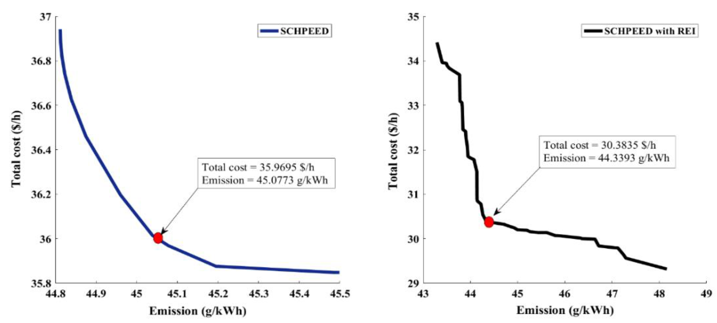
4.2.3. Best Compromise Solution
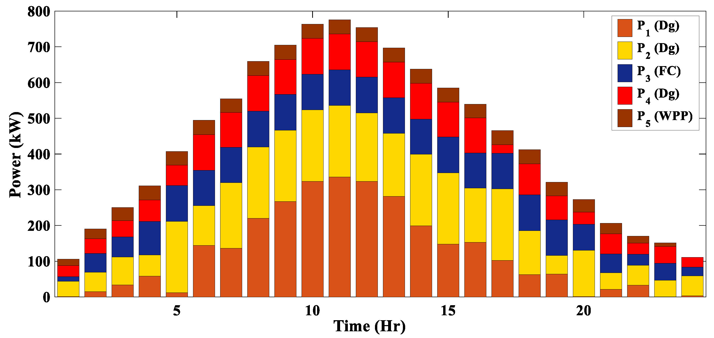
PPF is the weighted sum method to convert a multiobjective function into a single objective function. TOPSIS is used as a tool to rank the solution on the basis of the distance between positive and negative distance from the ideal solution. Table 7 and Table 8 show the top ten optimal front solutions for SCHPEED and MCHPEED problems. The elite solution was selected on the basis of top rank, and the corresponding Pareto fronts are shown in Figure 8, and Figure 9, respectively. Table 4 shows that for SCHPEED, the BCS in terms of the fuel cost of 35.9695 USD/h and the emission of 45.0773 g/kWh was also found to be superior to the reported results by DE [32] and PSO [32]. Considering Table 5, the BCS of 30.3835 USD/h and 44.3393 g/kWh was found to be lower due to REI with a topsis rank of 0.7886 as in Table 7.
For the MCHPEED problem, the BCS with the highest rank of 0.7602 (Table 8) in terms of cost and emission was found to be USD 1211.5507 and1077.6050 g/KW, respectively.
In the case of MCHPEED with REI, total cost refers to the sum of operational costs due to fossil fuel and renewable energy resources or both. Here, the total cost of USD 1094.9539 and the emission of 1050.8518 g/kW achieved the highest topsis rank of 0.7741, considered as BCS, as shown in Table 8. Here, it was observed that the operational cost was reduced by USD 113.5980 (9.4%), and the emitted emission was reduced by 26.7532 g/kW (2.5%) due to REI. The comparison of Pareto fronts is shown in Figure 8.

4.2.4. Heat Output

As shown in Table 9, considering the hourly load demand and corresponding heat output, it was observed that heat outputs were sensitive to changes in load demand. For the MCHPEED problem, heat output was seen to be increasing and fulfilled by energy resources with an increase in load demand.
However, considering Table 10 of MCHPEED with REI, it was observed that heat outputs remained increasing with load demand but were found to be lower as compared to MCHPEED. It may be due to sharing the particular range of load demand by renewable energy resources such as fuel cells and wind turbines.

5. Conclusions

In this paper, HHO successfully implements the planning of an MG to determine the optimal size and location of DGs and solve SCHPEED and MCHPEED problems to fulfill the particular load demand and a corresponding range of heat demand by different energy resources. The impact of REI is also investigated in both cases. Fuel cell and stochastic wind power are considered for analysis. TOPSIS is considered as a tool to obtain BCS based on the highest satisfaction level among the conflicting objectives. While comparing simulation results for the SCHPEED problem, the results obtained by HHO are found to be better compared to PSO and DE for minimum cost, minimum emission, and BCS for the multiobjective problem. The key findings are summarized below:
  • HHO is simple to implement and found to be impactful for the solution of both SCHPEED and MCHPEED complex constrained optimization problems.
  • With REI, fuel cost is reduced by 6.53 USD/h (18%) and emission is reduced by 1.519 g/kWh(3.4%) for SCHPEED, whereas fuel cost is reduced by USD 179.759 (14.95%) and emission is reduced by 59.60 g/kW (5.58%) for MCHPEED.
  • Heat output is found to be sensitive to changes in load demand
  • Operational cost, emission, and heat output are minimized with REI.

Author Contributions

Conceptualization, V.T. and H.M.D.; methodology, M.P.; software, S.R.S.; validation, V.T., H.M.D., and M.P.; formal analysis, S.R.S.; investigation, V.T.; resources, H.M.D.; data curation, M.P.; writing—original draft preparation, V.T. and H.M.D.; writing—review and editing, H.M.D., M.P., and S.R.S.; visualization, V.T.; supervision, M.P. and S.R.S.; project administration, V.T. and H.M.D.; funding acquisition, M.P. and S.R.S. All authors have read and agreed to the published version of the manuscript.

Funding

WOOSONG UNIVERSITY’s Academic Research Funding—2022.

Institutional Review Board Statement

Not applicable.

Informed Consent Statement

Not applicable.

Data Availability Statement

Not applicable.

Acknowledgments

The authors acknowledge the support provided by WOOSONG UNIVERSITY’s Academic Research Funding—2022.

Conflicts of Interest

The authors declare no conflict of interest.

Nomenclature

FCFuel cellRDSRadial distribution system
DGdistributed generatorsCHP Combined heat and power
MGmicrogridEED Economic emission dispatch
WPPWind power plantSCHPEEDCHP under EED for static (fixed) load
MTMicro TurbineMCHPEEDCHP under EED for Multiple (dynamic) load
REI Renewable Energy IntegrationBCSBest compromise solution
k p penalty cost due to underestimation of wind p d f Probability distribution function
k r reserve cost due to overestimation of wind V m i n   ,   V m a x Minimum and maximum voltage
k shape factor F D G T ,   F W P P T ,   F F C T cost of thermal units, wind power plant, and fuel cell, respectively
c scale factor v c i n , ,   v c o , v r Cut-in velocity, cut-out velocity, and rated velocity in m/s, respectively
H R Total heat output θ i Heat-to-power ratio of ith DG unit
H D Total heat demand. f 1 ,   f 2 Cost and emission function
P f n Price penalty factor w Weighting factor

References

  1. Alam, M.S.; Arefifar, S.A. Energy Management in Power Distribution Systems: Review, Classification, Limitations and Challenges. IEEE Access 2019, 7, 92979–93001. [Google Scholar] [CrossRef]
  2. Alipour, M.; Mohammadi-Ivatloo, B.; Zare, K. Stochastic scheduling of renewable and CHP-based microgrids. IEEE Trans. Ind. Infor. 2015, 11, 1049–1058. [Google Scholar] [CrossRef]
  3. Haghrah, A.; Nazari-Heris, M.; Mohammadi-ivatloo, B. Solving combined heat and power economic dispatch problem using real coded genetic algorithm with improved mühlenbein mutation. Appl. Therm. Eng. 2016, 99, 465–475. [Google Scholar] [CrossRef]
  4. Hagh, M.T.; Teimourzadeh, S.; Alipour, M.; Aliasghary, P. Improved group search optimization method for solving CHPED in large scale power systems. Energy Convers Manag. 2014, 80, 446–456. [Google Scholar] [CrossRef]
  5. Roy, P.K.; Paul, C.; Sultana, S. Oppositional teaching learning based optimization approach for combined heat and power dispatch. Int.J. Electr. Power Energy Syst. 2014, 57, 392–403. [Google Scholar] [CrossRef]
  6. Basu, M. Modified Particle Swarm Optimization for Non-smooth Non-convex Combined Heat and Power Economic Dispatch. Electr. Power Compon. Syst. 2015, 43, 2146–2155. [Google Scholar] [CrossRef]
  7. Lashkar Ara, A.; Mohammad Shahi, N.; Nasir, M. CHP Economic Dispatch Considering Prohibited Zones to Sustainable Energy Using Self-Regulating Particle Swarm Optimization Algorithm. Iran. J. Sci. Technol.—Trans. Electr. Eng. 2020, 44, 1147–1164. [Google Scholar] [CrossRef]
  8. Nguyen, T.T.; Vo, D.N.; Dinh, B.H. Cuckoo search algorithm for combined heat and power economic dispatch. Inter. J Electr. Power Energy Syst. 2016, 81, 204–214. [Google Scholar] [CrossRef]
  9. Beigvand, S.D.; Abdi, H.; La Scala, M. Combined heat and power economic dispatch problem using gravitational search algorithm. Electr. Power Syst. Res. 2016, 133, 160–172. [Google Scholar] [CrossRef]
  10. Ghorbani, N. Combined heat and power economic dispatch using exchange market algorithm. Inter. J.Electr. Power Energy Syst. 2016, 82, 58–66. [Google Scholar] [CrossRef]
  11. Basu, M. Group search optimization for combined heat and power economic dispatch. Inter. J.Electr. Power Energy Syst. 2016, 78, 138–147. [Google Scholar] [CrossRef]
  12. Jayakumar, N.; Subramanian, S.; Ganesan, S.; Elanchezhian, E.B. Grey wolf optimization for combined heat and power dispatch with cogeneration systems. Inter. J.Electr. Power Energy Syst. 2016, 74, 252–264. [Google Scholar] [CrossRef]
  13. Dashtdar, M.; Flah, A.; Hosseinimoghadam, S.M.; Kotb, H.; Jasińska, E.; Gono, R.; Leonowicz, Z.; Jasiński, M. Optimal Operation of Microgrids with Demand-Side Management Based on a Combination of Genetic Algorithm and Artificial Bee Colony. Sustainability 2022, 14, 6759. [Google Scholar] [CrossRef]
  14. Chiñas-Palacios, C.; Vargas-Salgado, C.; Aguila-Leon, J.; Hurtado-Pérez, E. A Cascade Hybrid PSO Feed-Forward Neural Network Model of a Biomass Gasification Plant for Covering the Energy Demand in an AC Microgrid. Energy Convers. Manag. 2021, 232, 113896. [Google Scholar] [CrossRef]
  15. Aguila-Leon, J.; Chiñas-Palacios, C.; Garcia, E.X.M.; Vargas-Salgado, C. A Multimicrogrid Energy Management Model Implementing an Evolutionary Game-Theoretic Approach. Int. Trans. Electr. Energy Syst. 2020, 30, e12617. [Google Scholar] [CrossRef]
  16. Barbosa-Ayala, O.I.; Montañez-Barrera, J.A.; Damian-Ascencio, C.E.; Saldaña-Robles, A.; Alfaro-Ayala, J.A.; Padilla-Medina, J.A.; Cano-Andrade, S. Solution to the Economic Emission Dispatch Problem Using Numerical Polynomial Homotopy Continuation. Energies 2020, 13, 4281. [Google Scholar] [CrossRef]
  17. Ahmadi, A.; Moghimi, H.; Nezhad, A.E.; Agelidis, V.G.; Sharaf, A.M. Multiobjective economic emission dispatch considering combined heat and power by normal boundary intersection method. Electr. Power Syst. Res. 2015, 129, 32–43. [Google Scholar] [CrossRef]
  18. Shaabani, Y.A.; Seifi, A.R.; Kouhanjani, M.J. Stochastic multiobjective optimization of combined heat and power economic/emission dispatch. Energy 2017, 141, 1892–1904. [Google Scholar] [CrossRef]
  19. Jayakumar, N.; Subramanian, S.; Ganesan, S.; Elanchezhian, E.B. Combined heat and power dispatch by grey wolf optimization. Inter. J. Energy Sect. Manag. 2015. [Google Scholar] [CrossRef]
  20. Sundaram, A. Multiobjective multi-verse optimization algorithm to solve combined economic, heat and power emission dispatch problems. Appl. Soft Comp. 2020, 91, 106195. [Google Scholar] [CrossRef]
  21. Dubey, H.M.; Pandit, M.; Panigrahi, B.K. An overview and comparative analysis of recent bio-inspired optimization techniques for wind integrated multiobjective power dispatch. Swarm Evol Comp. 2018, 38, 12–34. [Google Scholar] [CrossRef]
  22. Basu, M.; Chowdhury, A. Cuckoo search algorithm for economic dispatch. Energy 2013, 60, 99–108. [Google Scholar] [CrossRef]
  23. Basu, M. Squirrel Search Algorithm for Multi-region Combined Heat and Power Economic Dispatch Incorporating Renewable Energy Sources. Energy 2019, 182, 296–305. [Google Scholar] [CrossRef]
  24. Dubey, S.M.; Dubey, H.M.; Pandit, M.; Salkuti, S.R. Multiobjective Scheduling of Hybrid Renewable Energy System Using Equilibrium Optimization. Energies 2021, 14, 6376. [Google Scholar] [CrossRef]
  25. Jin, J.; Wen, Q.; Zhang, X.; Cheng, S.; Guo, X. Economic Emission Dispatch for Wind Power Integrated System with Carbon Trading Mechanism. Energies 2021, 14, 1870. [Google Scholar] [CrossRef]
  26. Vargas-Salgado, C.; Berna-Escriche, C.; Escrivá-Castells, A.; Díaz-Bello, D. Optimization of All-Renewable Generation Mix According to Different Demand Response Scenarios to Cover All the Electricity Demand Forecast by 2040: The Case of the Grand Canary Island. Sustainability 2022, 14, 1738. [Google Scholar] [CrossRef]
  27. Tiwari, V.; Dubey, H.M.; Pandit, M. Economic Dispatch in Renewable Energy Based Microgrid Using Manta Ray Foraging Optimization. In Proceedings of the 2nd International Conference on Electrical Power and Energy Systems (ICEPES 2021), Online Mode, 10–11 December 2021; pp. 1–6. [Google Scholar] [CrossRef]
  28. Harsh, P.; Das, D. Energy Management in Microgrid Using Incentive-Based Demand Response and Reconfigured Network Considering Uncertainties in Renewable Energy Sources. Sustain. Energy Technol. Assess. 2021, 46, 101225. [Google Scholar] [CrossRef]
  29. Anand, H.; Narang, N.; Dhillon, J.S. Multi-Objective Combined Heat and Power Unit Commitment Using Particle Swarm Optimization. Energy 2019, 172, 794–807. [Google Scholar] [CrossRef]
  30. Rezaee Jordehi, A. A Mixed Binary-continuous Particle Swarm Optimisation Algorithm for Unit Commitment in Microgrids Considering Uncertainties and Emissions. Int. Trans. Electr. Energy Syst. 2020, 30, e12581. [Google Scholar] [CrossRef]
  31. Hetzer, J.; Yu, D.C.; Bhattarai, K. An economic dispatch model incorporating wind power. IEEE Trans. Energy Convers 2008, 23, 603–611. [Google Scholar] [CrossRef]
  32. Basu, A.K.; Bhattacharya, A.; Chowdhury, S.; Chowdhury, S.P. Planned scheduling for economic power sharing in a CHP-based micro-grid. IEEE Tran. Power Syst. 2011, 27, 30–38. [Google Scholar] [CrossRef]
  33. Wolpert, D.H.; Macready, W.G. No free lunch theorems for optimization. IEEE Trans. Evol. Comp. 1997, 1, 67–82. [Google Scholar] [CrossRef] [Green Version]
  34. Heidari, A.A.; Mirjalili, S.; Faris, H.; Aljarah, I.; Mafarja, M.; Chen, H. Harris hawks optimization: Algorithm and applications. Future Gener. Comput. Syst. 2019, 97, 849–872. [Google Scholar] [CrossRef]
  35. Abdelsalam, M.; Diab, H.Y.; El-Bary, A.A. A Metaheuristic Harris Hawk Optimization Approach for Coordinated Control of Energy Management in Distributed Generation Based Microgrids. Appl. Sci. 2021, 11, 4085. [Google Scholar] [CrossRef]
  36. Hong, L.; Rizwan, M.; Rasool, S.; Gu, Y. Optimal Relay Coordination with Hybrid Time–Current–Voltage Characteristics for an Active Distribution Network Using Alpha Harris Hawks Optimization. Eng. Proc. 2021, 12, 26. [Google Scholar] [CrossRef]
  37. Hwang, C.L.; Yoon, K.P. Multiple Attribute Decision Making: Methods and Applications; Springer: New York, NY, USA, 1981. [Google Scholar] [CrossRef]
Figure 1. Different phases of HHO.
Fluids 07 00248 g001
Figure 2. Flowchart of HHO algorithm.
Fluids 07 00248 g002
Figure 3. Single line diagram of 14-bus RDS.
Fluids 07 00248 g003
Figure 4. The generation scheduling of MSCHPEED for cost minimization.
Fluids 07 00248 g004
Figure 5. The generation scheduling of MSCHPEED with REI for cost minimization.
Fluids 07 00248 g005
Figure 6. The generation scheduling of MSCHPEED for emission minimization.
Fluids 07 00248 g006
Figure 7. The generation scheduling of MSCHPEED with REI for emission minimization.
Fluids 07 00248 g007
Figure 8. Pareto optimal fronts for SCHPEED and SCHPEED with REI.
Fluids 07 00248 g008
Figure 9. Pareto optimal fronts for MCHPEED and MCHPEED with REI.
Fluids 07 00248 g009
Table 1. Line and load data of 14-bus RDS.
Bus No.Start BusEnd BusRXRealReactive
1000000
2120.01330.042206
3230.01940.0598527
4340.03120.16401
5250.0230.12206
6560.0230.12206
7670.01930.0597616
8680.0320.0841030
9790.0340.176116
102100.0160.0421275
1110110.1930.0591090
1211120.0670.171661
1312130.040.19059
1411140.050.153561
Table 2. Simulation results for 14-bus RDS.
ParametersWithout DGsWith 4 DGs
Power Loss (kW)0.19950.1297
Loss Reduction (%)-34.99
DGs Size (kW) /Location-90.3178/3, 187.9/7, 114.9414/13, 44.8314/14
Total DG Size (kW)-437.9906
V m i n (pu)0.99920.9995
V m a x (pu)0.99980.9999
Table 3. Operational limits, fuel cost coefficient, emission coefficient, and heat rate data.
Type Size   ( k W ) P i m i n
( k W )
P i m a x
( k W )
a i b i c i α i β i γ i H e a t   R a t e  
( k j / k W h )
Dg5000.0050010.193105.1862.5626.55−16.18367.050810,314
Dg200402002.03560.2844.014.4296−64.1535130.409411,041
MT8016800.576857.783−133.09153.0358−57.3403311.572811,373
Dg100201001.182565.3444.019.38−176.6946821.657310,581
MT306.0300.33889.1476−547.6191.0346−60.384943.189812,186
FC100010000.0700000
WPP4004000.2200000
Table 4. Generation schedule and comparative results for SCHPEED with demands of 338 kW.
ScenariosMethods P 1 ( D g ) P 2 ( D g ) P 3 ( M T ) P 4 ( D g ) P 5 ( M T ) Fuel Cost (USD/h)Emission (g/kWh)Heat (kWh)Loss (kW)
Best CostHHO0.00157.0980.0073.155230.0035.848345.4856347.56392.2452
DE [32]0.00166.3080.0064.3030.0035.897445.8467348.048---
PSO [32]0.00166.6880.0063.8930.0035.89745.870348.000---
Best EmissionHHO0.00168.800957.184896.054021.052636.939644.8121329.36945.0922
DE [32]0.00166.5058.3096.1021.5036.85144.820329.790---
PSO [32]0.00166.2058.6496.0721.6636.84044.820330.070---
BCSHHO0.00146.431280.0089.9224.765635.969545.0773344.06853.1168
DE [32]0.00150.5480.0090.9220.5536.072045.020341.7225---
PSO [32]0.00150.2080.0089.8621.9536.060045.030342.7200----
BCS: Best Compromise Solution.
Table 5. Generation schedule and comparative results for SCHPEED with REI with demands of 338 kW.
Scenario P 1 ( D g ) P 2 ( D g ) P 3 ( F C ) P 4 ( D g ) P 5 ( W P P ) Total Cost (USD/h)Fuel Cost (USD/h)Wind Cost (USD/h)Emission (g/kWh)Heat (kWh)Loss (kW)
Best Cost0.00174.842595.631833.269439.874129.318027.52521.792848.1604171.18455.6179
Best Emission0.00200.0050.1720100.000.467034.411434.20400.207443.2924244.972512.6390
BCS0.00155.068792.043688.69009.144830.383529.96380.419744.3393198.79076.9470
Table 6. Comparative results for MCHPEED and MCHPEED with REI.
ScenarioMCHPEEDMCHPEED with REI
Total Cost
(USD)
Emission
(g/kW)
Heat
(kW)
Loss
(kW)
Total Cost
(USD)
Fuel Cost
(USD)
Wind Cost
(USD)
Emission
(g/kW)
Heat
(kW)
Loss
(kW)
Min.Cost1203.09991089.925615,587.8723203.56411023.34031003.246520.09381085.853215,528.2799167.1917
Min. Emis1250.00661068.156715,918.5405309.10871384.19951361.90222.29751008.549017,674.5642555.1573
BCS1211.55071077.605015,588.9110212.68141094.95391070.960223.99371050.851815,579.2478253.8731
Table 7. Top ten Pareto optimal solution for SCHPEED.
S. No.SCHPEEDSCHPEED with REI
Fuel Cost
(USD/h)
Emission
(g/kWh)
M u 1 M u 2 TOPSISTotal Cost
(USD/h)
Emission
(g/kWh)
M u 1 M u 2 TOPSIS
135.969545.07730.0020.00790.79630.383544.33930.01110.04150.7886
236.014845.03890.0020.00770.794130.539644.22420.01170.0410.7784
335.876645.19440.00260.00830.761330.014745.19520.0140.04070.7433
436.197444.960.00280.00670.703930.245945.26670.01530.03880.7172
535.848345.48560.00460.00830.643630.384345.3360.01630.03760.698
636.459744.87530.00460.00560.546431.510143.94870.01820.03680.6697
736.626144.83940.00590.00510.463331.408644.4440.01850.03490.6531
836.740544.82320.00680.00480.417731.854344.18040.02130.03390.6146
936.825844.81570.00740.00470.390129.644947.29350.02720.03880.5877
1036.939644.81210.00830.00470.361429.31848.16040.03290.0410.5542
Table 8. Top ten optimal front solutions.
S. No.MCHPEEDMCHPEED with REI
Fuel Cost
(USD)
Emission
(g/kW)
M u 1 M u 2 TOPSISTotal Cost
(USD)
Emission
(g/kW)
M u 1 M u 2 TOPSIS
11211.5511077.6050.03420.10840.76021094.9541050.8520.15510.53130.7741
21216.5661072.8380.03810.10150.72681137.6641039.9210.21880.45760.6765
31216.9211074.5780.04060.09880.7091175.7551033.9770.28410.39240.58
41203.11089.9260.05610.12410.68881199.7081030.5570.32630.35220.5191
51221.7141073.9120.05090.08910.63651228.0731028.5830.37720.30450.4467
61222.01871082.32970.0440.05780.56771260.9821023.5430.43620.25370.3677
71223.1821087.87930.05220.05420.50931280.7611022.4090.47210.22360.3214
81227.42041086.41620.0560.04710.45681306.8191015.0370.5190.19470.2728
91230.06981089.84650.06350.04210.39831347.691013.7010.59340.15210.204
101250.0071068.1570.11730.0570.32721384.21008.5490.65980.14650.183
Table 9. Optimal generation scheduling for MCHPEED under BCS.
Hr. P 1 ( D g ) P 2 ( D g ) P 3 ( M T ) P 4 ( D g ) P 5 ( M T ) Load (kW)Heat (kW)
10.174243.822618.9528.948413.7722105107.6286
20.0439100.222220.899657.296715.1846190181.4153
37.9917106.520341.902682.854915.4974250257.7412
434.649686.604179.719795.891416.1365310375.0671
579.0714122.396476.641798.917125.9711400532.2534
6111.5772186.894379.595291.347924.9627490666.1347
7146.7594199.992778.847899.859329.8921550780.8991
8256.9116199.668677.206199.998229.13316501061.2783
9300.363199.938679.999899.726428.94616901177.0124
10364.7395199.125678.174999.979828.66317401339.5097
11377.743420079.986498.319427.77667501373.6715
12353.816197.543979.968710027.35657301310.6095
13292.299196.90378.459499.9998306801153.3381
14232.1257199.73088099.89228.65246301000.5748
15183.5236198.066378.552697.059329.4762580870.8251
16173.3918175.396664.503699.933127.4251535805.1119
17137.2064147.806478.367779.065121.3752460682.8948
1899.7382139.122167.809285.651520.4403410567.8843
1959.861375.393279.43389.888417.4494320427.6205
201.3002129.098656.305576.806311.8101270269.2425
216.21692.059222.551177.349111.2522205202.8413
222.980372.956333.592552.341110.0549170172.7066
23058.097331.354553.86458.5012150148.3782
244.662741.223827.901423.527512.9832110124.272
Table 10. Optimal generation scheduling for MCHPEED with REI under BCS.
Hr. P 1 ( D g ) P 2 ( D g ) P 3 ( F C ) P 4 ( D g ) P 5 ( W P P ) Load (kW)Heat (kW)
10.460255.80010.002638.109212.208710577.6358
20.001467.209932.684976.963316.9728190116.7346
316.605176.360749.98597.699313.7738250183.5804
443.870295.402665.2486.562221.4451310260.8134
52.0257193.151484.199299.909531.4198400244.4528
6137.9878156.381994.301581.560423.9735490550.0218
7172.6773181.974383.465484.742733.0027550663.1865
8248.3451198.683988.241397.609929.5584650882.3438
9339.0121193.14390.5573.611523.3266901092.496
10389.558193.496693.755785.528117.99757401232.578
11372.8658192.926695.047896.245727.39947501197.57
12365.0877198.161372.758687.81137.27457301175.156
13288.2583183.185895.287996.536234.9216680971.5743
14238.2183198.167183.906183.290437.8205630844.4403
15198.0663199.998668.834984.558235.8806580743.4311
16161.1864184.682970.223289.780634.1974535639.7981
1798.8017154.43688.227292.892928.9415460456.3623
1833.2158174.075376.476799.999433.2225410309.1514
1916.428103.646867.959797.065939.9701320205.216
2015.2292136.688229.952962.314430.3556270201.9077
21059.101439.974190.144320.5677205120.4767
229.531678.9362.698264.958717.4007170141.4918
231.300647.400842.515851.39218.648215083.3885
240.267560.301312.160936.16352.382911079.3222
Publisher’s Note: MDPI stays neutral with regard to jurisdictional claims in published maps and institutional affiliations.

