
Periodic and Solitary Wave Solutions of the Long Wave–Short Wave Yajima–Oikawa–Newell Model
by
 , , , and
Marcos Caso-Huerta
1,† ,
,
Antonio Degasperis
2,†,
Priscila Leal da Silva
3,4,†,
Sara Lombardo
3,*,† and
Matteo Sommacal
1,† 1
Department of Mathematics, Physics and Electrical Engineering, Northumbria University, Newcastle upon Tyne NE1 8ST, UK
2
Department of Physics, ‘Sapienza’ Università di Roma, 00185 Rome, Italy
3
Department of Mathematical Sciences, School of Science, Loughborough University, Loughborough LE11 3TU, UK
4
Centre of Mathematics, Computation and Cognition, Universidade Federal do ABC, Santo André 09210-580, Brazil
*
Author to whom correspondence should be addressed.
†
These authors contributed equally to this work.
Fluids 2022, 7(7), 227; https://doi.org/10.3390/fluids7070227
Submission received: 10 June 2022
/
Revised: 26 June 2022
/
Accepted: 27 June 2022
/
Published: 4 July 2022
(This article belongs to the Special Issue Nonlinear Wave Hydrodynamics, Volume II)
Abstract
:Models describing long wave–short wave resonant interactions have many physical applications, from fluid dynamics to plasma physics. We consider here the Yajima–Oikawa–Newell (YON) model, which was recently introduced, combining the interaction terms of two long wave–short wave, integrable models, one proposed by Yajima–Oikawa, and the other one by Newell. The new YON model contains two arbitrary coupling constants and it is still integrable—in the sense of possessing a Lax pair—for any values of these coupling constants. It reduces to the Yajima–Oikawa or the Newell systems for special choices of these two parameters. We construct families of periodic and solitary wave solutions, which display the generation of very long waves. We also compute the explicit expression of a number of conservation laws.
1. Introduction
The study of wave propagation poses quite a number of challenging different mathematical and computational problems [1].
The wave motion of continuous media is generally represented by solutions of one or more partial differential equations (PDEs). Typically, homogeneous wave propagation equations have a linear part, which is characterized by a dispersion law, and a nonlinear one, which is responsible for self and/or cross interaction. While the linear part can be treated by decomposition into Fourier harmonics, the nonlinear part—even if its dependence on the fields is analytic—is generically treatable only by numerical methods. These two parts, in terms of solvability, recombine in cooperation with each other for a small set of very special wave equations, the so-called integrable ones, by allowing for a sort of nonlinear Fourier-like analysis [2,3].
We have in mind (and consider below) only waves propagating in a one-dimensional space, even if integrable wave equations in higher dimension are known too. Since their first discovery more than half a century ago, the firmament of integrable wave equations has been continuously growing. From the very beginning, water waves have played a pivotal role in this research, with the discovery of the integrability of the Boussinesq equation, the Korteweg–de Vries (KdV) equation and the nonlinear Schrödinger (NLS) equation, which may serve as approximate models of waves traveling on a water-free surface subject to various physical conditions.
The existence of solitons is the most celebrated and effective prediction from the study of water wave equations of integrable type. Subsequent research has pointed out that discovering integrable wave equations is not only due to a lucky strike in the process of approximating complicated PDEs of physical significance. In fact, integrable models can be obtained by means of a perturbation approach, the so-called multiscale method (see [4,5,6]), when applied to a given known nonlinear wave equation. Indeed, given a physically relevant PDE, by appropriately rescaling both wave amplitudes and space–time coordinates via the introduction of a small parameter , and by expanding in powers of , one ends up with a different PDE which models the amplitude modulation in the rescaled space–time coordinates. The point is that this process preserves the integrability property of the original wave equation and thus it yields a (possibly) new integrable wave equation. The rationale behind this method is based on physical arguments: one considers the nonlinear terms as a perturbation of known Fourier-like solutions (harmonics) of the linear dispersive part. Consequently, approximate solutions of the original PDE look like superpositions of exponentials as, for instance, , whose amplitudes depend on rescaled coordinates only. The parameters k and are the wave number and frequency on the dispersion curve . If the superposition of harmonics contains more wave numbers, this multiscale method in general yields a system of coupled PDEs, which models wave–wave interactions.
A necessary condition for this to happen is the (weak) resonance relation:
Several models of resonant interaction have been derived in this way (e.g., see [5,6,7]) to investigate their main features by means of known integrability techniques, provided such models were selected as sufficiently “close” to a wave equation of specific physical interest.
This perturbative approach is also appropriate to investigate the resonant coupling of two quasi-monochromatic waves, one with very long wave-length, say, with wave number , and the second one with a much shorter wave-length, say with wave number . As originally pointed out in [8], this interaction can be understood as a resonant triad , , , namely
with
Indeed, if the long wave is sufficiently long, say , and the dispersion function is analytic at , this condition is equivalent to the stronger condition that the long wave and the short wave have the same group velocity, .
The search for integrable PDEs which reasonably model phenomena due to long wave–short wave (L-S) interaction started in the early years of the soliton era in fluid dynamics, plasma physics and optics. The Yajima–Oikawa (YO) system [9]
was first derived in the one-way wave approximation in plasma. Here and in the following, S and L are the complex, and, respectively, real amplitudes of the short and long waves. This system shows up also via the multiscale technique [7] in multiple ways. In fact, it proves to be a multiscale reduction of an integrable equation of interest in water waves, namely the Boussinesq equation [5]. A second and alternative integrable L-S wave system was proposed by Newell [10]. This one reads
where, in addition to a long wave–short wave coupling, the short wave has the same self-interaction as the NLS equation, which may be both defocusing or focusing according to the sign . We will refer to the system (2) as to the N equation. However, the way to obtain this system as a multiscale reduction of an integrable equation does not seem to be known.
In [11], it was shown that the YO and N Equations (1) and (2) need not be separately treated to investigate the short wave–long wave interaction. Indeed, these two different model equations, remarkably enough, can be combined in just one system, which we refer to as the YON model, that is itself integrable for any real value of the two arbitrary parameters and , namely
This system coincides with the YO Equation (1) for , , while it reads as the N Equation (2) by setting , and by substituting the field L with . This unifying result provides a greater flexibility in modeling the resonant interaction of long and short waves, and allows to construct and analyze in one go the special solutions of the two models, (1) and (2). On the mathematical side, we note that the YON model (3) turns out to be a reduction of a larger system of four coupled PDEs [12].
The preliminary step to inquire on the application of the YON system to specific physical wave phenomena is the compatibility of the L-S resonance condition (see the triad resonance above) with the dispersion law (for an instance of such analysis in optics, see [13]). Having in mind a fluid dynamical context, we recall a few elementary facts to show that water waves on the free surface of a two-dimensional rectangular container require that gravity be contrasted by surface tension [14]. Indeed, this effect allows the resonance, which, however – at least in geophysical applications—is far from being of experimental relevance; see [15]. As it happens, if the surface tension is neglected, the dispersion law
where g is the gravity acceleration and h is the depth of the flat bottom, does not allow for the L-S resonance since the group velocity is monotonically decreasing in the entire range . Surface tension, if the wave length is sufficiently short, may contrast gravity and change the dispersion law into
where is the surface tension constant and is the water density. Although this change of the frequency dispersion formally allows for the S-L resonance, the value of which satisfies the strong resonance condition strongly depends on the depth h. For instance, a short wave of about length requires a flat bottom of approximately depth. For stratified fluids, see for instance [16,17].
Despite such resonant conditions leading to small effects in capillarity–gravity wave propagation, we deem it of interest to investigate the YON model because of its potential applicability while being integrable. Indeed, it has been shown [11] that there exists a Lax pair of equations for an auxiliary function (where is a complex number called spectral parameter or spectral variable)
whose compatibility condition
is equivalent to the YON system (3). Here and are complex matrix-valued functions depending on the field variables S and L, and also polynomially on the spectral variable ,
where and denote constant, traceless, diagonal matrices
and the matrices , and have the form
However, in the following, we will not make use of the Lax pair (4), and we refer the interested reader to [11], where further details on the integrable character of the system can be found.
In the next section, we discuss several families of periodic and traveling wave solutions of the YON system (3), including dark and bright solitons, as well as rational solitons. Finally, in Section 3, using a set of multipliers, we construct and exhibit a family of conservation laws. To this purpose, it is instrumental the use of symmetry transformations of our system (3). Thus we end this section by observing that the YON system (3) is trivially invariant with respect to translations in space and time, as well as to rotations around the origin in the S plane. Moreover, the YON system is invariant under the general transformation
where is an arbitrary parameter. Note that the limit of the above transformation can be obtained by mapping first. If , we have that (3), namely the YO system (1), is invariant under the additional scaling:
while, if , say if (3) is the N system (2), the invariant scaling transformation is
where is an arbitrary parameter.
2. Solutions of the YON Model
Although system (3) is integrable and hence it allows for solutions to be found by a variety of elegant and powerful solution techniques rooted into integrability theory, for the purpose of this paper, we use instead an Ansatz to derive periodic and traveling wave solutions, without resorting to heavier mathematical machineries. Our Ansatz naturally follows the form of the periodic and traveling wave solutions of the nonlinear Schrödinger equation, and it reads
where for , , and s, , ℓ are real valued functions. After substitution of the Ansatz into the second equation of (3), the resulting equation can be integrated in order to obtain ℓ in terms of s:
where is an arbitrary integration constant. We now make use of this new expression for L, substitute in the first equation of (3) and separate it into real and imaginary parts in order to obtain the system
for the functions s and . Equation (10a) can be integrated with respect to z after multiplication by s, yielding an expression for the first derivative of in terms of s:
where is an integration constant. We now plug this expression for into Equation (10b), obtaining
Equation (12) can be integrated with respect to z after multiplication by , resulting in a differential equation for :
where is an integration constant. Observe that for , the coefficient of becomes zero and the equation simplifies, leading to the Weierstraß elliptic function. The case corresponds to the YO model, well studied in the literature, e.g., see [18,19] for some recent results about periodic and rational solutions and the literature therein.
Here and thereafter, we will assume . Introducing the following change of variable
Equation (13) becomes, without any loss of generality,
where
whereas c, , and are arbitrary constants. Note that the number of arbitrary constants is preserved. The integration constants , and can be rewritten in terms of c, and as follows:
As for , from (11), we obtain the quadrature
For , Equation (15) admits periodic solutions in terms of Jacobi elliptic functions, which we discuss below.
2.1. Jacobi Elliptic Sine Solution
Let us assume that has the form
where denotes the Jacobi elliptic sine of z, where , , a, and m are real parameters, and . Inserting (19) into (15) with and playing with the properties of the Jacobi elliptic functions, one obtains a polynomial of degree four in equated to zero. Setting the coefficients of each power of to zero, one obtains a set of algebraic equations for the parameters , m, a, , , and c. In particular, a relation for in terms of the other parameters can be found by setting the constant term of the polynomial to zero. This latter relation returns a non-real for any choice of the other parameters, and therefore, this excludes the existence of a sn-solution of the form (19) starting from Ansatz (8).
2.2. Jacobi Elliptic Cosine Solution
Proceeding as above but with the Jacobi elliptic cosine replacing in (19), we obtain the following solution to (15) in:
with
and
where m, , and b are real parameters, with . Replacing the expression of into the original Ansatz (8), we obtain the following solution of the YON system:
where satisfies the quadrature
where the sign in front of the square root is the same sign chosen for . Observe that, in addition to the coupling parameters and in the YON model (3), the solution (Section 2.2) features five real parameters, namely a, b, m, V and , with a sixth real, arbitrary parameter coming from the integration of (22c).
For this to work, we need s, , and to be real. In order to assure that, we need to check the sign inside all the square roots involved, which gives us constraints on the parameters, namely
Furthermore, in the special case , the value is allowed as long as ; see Section 2.4.
The short wave oscillates between the values
That is to say, oscillates with amplitude , while the long wave L oscillates between the values
that is, with amplitude . The cn-solution is periodic in x with period and in t with period , where is the complete elliptic integral of the first kind of m,
An example of cn-solution is illustrated in Figure 1.
Moreover, we observe that there are two special solutions corresponding to the particular choices and . If , the elliptic cosine reduces to the trigonometric cosine, and the solution becomes a plane wave. If the elliptic cosine reduces to the hyperbolic secant, leading to a localized solution, treated in Section 2.4.
2.3. Jacobi Delta Amplitude Solution
Proceeding as above with the Jacobi delta amplitude replacing in (19), we obtain the following solution to (15)
with
and
where m, , and b, are real parameters, with .
The solution in this case has the form
where satisfies the quadrature
where the sign in front of the square root is the same sign chosen for . Similar to the Jacobi elliptic solutions (Section 2.2), observe that the solutions (Section 2.3) feature five real parameters, namely a, b, m, V and , with a sixth real, arbitrary parameter coming from the integration of (27c).
Again, checking the square roots that appear for having real solutions, we obtain the following constraints on the parameters:
It also allows the special values and , for . We discuss the special case in Section 2.4.
The dn solution has periodicity for L and with period , where is the complete elliptic integral of the first kind of m, while the phase of S has a period .
The short wave oscillates between the values
That is to say, the oscillations in have an amplitude , while the long wave L oscillates between the values
that is, with an amplitude . An example of dn-solution is illustrated in Figure 2.
2.4. Traveling Waves: Solitons
The choice in (20) makes the period of the elliptic cosine diverge, so the solution becomes localized. The corresponding solutions are solitons, both of the dark and bright types.
The solution for , which for a generic choice of parameters corresponds to a dark soliton, has the form
with
where is an arbitrary phase, and the sign function satisfies . As a consequence of (23), and as it can be observed from the formulae above, the general condition on the parameters for the validity of the soliton solution, when , is
The special choice (see below) is also allowed by the system, though the resulting solution has the phase
The square of the short wave, , has an amplitude over the background , while the long wave L has an amplitude over the background . Note that both amplitudes and the background of S do not depend on at all, while they all depend inversely on .
By construction, both and are centered at , while and for a given are both centered at .
Whenever , S has zero background, and whenever , L has zero background too. Both equalities being true means having a bright soliton solution, both being false leads to a dark soliton solution, while the cases where one is true and the other is not lead to mixed bright–dark solutions.
The resulting formula for the bright case is
2.5. Traveling Waves: Rational Solution
Computing the integral, solving with respect to and substituting into the expressions for and leads to the solution
where is an arbitrary phase, and the constraint is assumed.
The short wave is a dark rational solution with an amplitude depression of propagating on the non-vanishing background , whereas the long wave L has an amplitude over the asymptotic background . An example of rational solution is illustrated in Figure 4.
In the case where and we are back to the Newell system (2), the solution is simplified to
where . To the best of our knowledge, this is the first time such a solution is derived for (2).
Another solution can be obtained for but now for , still with . The quadrature (13) is now rewritten as
and integration leads to the solutions
The short wave and long wave L are bright rational solutions with amplitudes of and , respectively, on a zero background. To the best of our knowledge, this is also a novel solution of (2).
3. Conservation Laws
The YON model (3) is integrable, and therefore it allows infinitely many conservation laws. In this section, we are interested in deriving a few explicit ones, by finding convenient multipliers. A conservation law of (3) corresponds to an expression
where is the density and the corresponding flux, respectively. For instance, a trivial conservation law of the YON system (3) is
which coincides with the second equation in (3).
In [20,21,22], it was established that every conservation law corresponds to a symmetry of the equation, but very often, this symmetry is non-classical or even non-local. For cases where Noether’s theorem is applicable, this correspondence is explicit, as Noether symmetries lead to (possibly trivial) conserved vectors; however, we ruled out this approach, as we were unable to find a variational formulation for system (3). Instead of using Noether’s approach, we consider the direct method illustrated in [20,21,22,23], consisting in finding a vector , called multiplier, that depends on S, L and their derivatives up to a certain fixed but arbitrary order, such that
where
and where is the variational derivative with respect to the variable u. If such a vector g can be found, then it ensures the existence of and f such that
4. Conclusions
Models describing long wave–short wave resonant interactions arise in a variety of physical contexts, from fluid dynamics to plasma physics. In this paper, we consider the recently proposed, long wave–short wave YON (Yajima–Oikawa–Newell) model (see [11]), an integrable model featuring two arbitrary parameters, and unifying and generalizing the Yajima–Oikawa model and the Newell model.
We studied some relevant families of periodic and solitary wave solutions, displaying the generation of very long waves. Among others, we also displayed the expression of solutions that we term, with some abuse of language, “rational”. Differently from the NLS equation, where the amplitude is indeed rational (cf., the Peregrine soliton), in the present case, it is rather the function that comes to be rational. This is due to the quintic nonlinearity appearing in the YON system for the short wave amplitude , rather then the usual cubic one as in the NLS equation. An analytical study of the stability of the solutions presented in this paper is left to future investigation. In this respect, we limit ourselves to report here that we carried out a preliminary numerical study, solving the initial value problem for initial conditions obtained by computing our solutions at , using the method of lines with pseudospectral, Fourier discretization in space and an adaptive Dormand–Prince embedded Runge–Kutta method for the time stepping: the numerical results seem to suggest the existence of regions of stability and regions where different forms of instability are observed, similar to what is predicted for plane wave solutions of the YON system [11,29].
The families of explicit solutions presented in this paper were obtained by choosing a suitable Ansatz. A systematic derivation of soliton solutions of bright, gray and dark types, as well as of breathers and rogue waves, exploiting the integrable character of the YON system, is currently in progress.
In this paper, we also derived a few conservation laws, which are of interest in view of the numerical and analytical studies of this system. An argument based on the effect of the surface tension on the dispersion relation for short waves, allowing for short–long wave resonance, is presented to justify the physical relevance of the YON model in a fluid-dynamical context (and in particular for experimental set-ups of capillarity–gravity wave propagation on the scales of the centimeters), where the value of the wave number strongly depends on the water depth. In spite of the expected physical relevance, a derivation, via multiscale techniques, of the full YON system—similar to the Newell model, which is contained within the YON system—as an (integrable) reduction from a known physical PDE has not yet been achieved and remains an intriguing open problem. It is worth observing that a subcase of the YON model, namely the Yajima–Oikawa model, has been indeed derived via the multiscale technique in more than one way [7], suggesting that this should be possible also for the more general YON model.
Author Contributions
Conceptualization, software, validation, formal analysis, investigation, writing—original draft preparation, writing—review and editing, M.C.-H., A.D., P.L.d.S., S.L. and M.S. All authors contributed equally to this work. All authors have read and agreed to the published version of the manuscript.
Funding
PLdS is supported by the Royal Society under a Newton International Fellowship (reference number 201625) hosted by SL.
Acknowledgments
SL and PLdS acknowledge support by the Royal Society. The work of MS has been carried out under the auspices of the Italian GNFM (Gruppo Nazionale Fisica Matematica), INdAM (Istituto Nazionale di Alta Matematica).
Conflicts of Interest
The authors declare no conflict of interest.
Appendix A. Conserved Vectors Depending on Derivatives up to the Second Order
References
- Whitham, G.B. Nonlinear dispersion of water waves. J. Fluid Mech. 1966, 27, 399–412. [Google Scholar] [CrossRef]
- Ablowitz, M.J.; Kaup, D.J.; Newell, A.C.; Segur, H. The inverse scattering transform-Fourier analysis for nonlinear problems. Stud. Appl. Math. 1974, 53, 249–315. [Google Scholar] [CrossRef]
- Calogero, F.; Degasperis, A. Spectral Transform and Solitons; North-Holland: Amsterdam, The Netherlands, 1982. [Google Scholar]
- Zakharov, V.E.; Kuznetsov, E.A. Multi-scale expansions in the theory of systems integrable by the inverse scattering transform. Physica D 1986, 18, 455–463. [Google Scholar] [CrossRef] [Green Version]
- Calogero, F. Why are certain nonlinear PDEs both widely applicable and integrable. In What is Integrability? Zakharov, V.E., Ed.; Springer: Berlin/Heidelberg, Germany, 1991. [Google Scholar]
- Degasperis, A. Multiscale expansion and integrability of dispersive wave equations. In Integrability; Lecture Notes in Physics; Mikhailov, A.V., Ed.; Springer: Berlin/Heidelberg, Germany, 2009; Volume 767, pp. 215–244. [Google Scholar]
- Calogero, F.; Degasperis, A.; Xiaoda, J. Nonlinear Schrödinger-type equations from multiscale reduction of PDEs. I. Systematic derivation. J. Math. Phys. 2000, 41, 6399–6443. [Google Scholar] [CrossRef]
- Benney, D.J. A general theory for interactions between short and long waves. Stud. Appl. Math. 1976, 56, 81–94. [Google Scholar] [CrossRef]
- Yajima, N.; Oikawa, M. Formation and interaction of sonic-Langmuir solitons: Inverse scattering method. Prog. Theor. Phys. 1976, 56, 1719–1739. [Google Scholar] [CrossRef] [Green Version]
- Newell, A.C. Long waves-short waves: A solvable model. SIAM J. Appl. Math. 1978, 35, 650–664. [Google Scholar] [CrossRef]
- Caso-Huerta, M.; Degasperis, A.; Lombardo, S.; Sommacal, M. A new integrable model of long wave-short wave interaction and linear stability spectra. Proc. R. Soc. A 2021, 477, 20210408. [Google Scholar] [CrossRef]
- Wright, O.C. Homoclinic connections of unstable plane waves of the long-wave–short-wave equations. Stud. Appl. Math. 2006, 117, 71–93. [Google Scholar]
- Chowdhury, A.; Tataronis, J.A. Long-wave short-wave resonance in nonlinear negative refractive index media. Phys. Rev. Lett. 2008, 100, 153905. [Google Scholar] [CrossRef]
- Djordjevic, V.D.; Redekopp, L.G. On two-dimensional packets of capillary-gravity waves. J. Fluid Mech. 1977, 79, 703–714. [Google Scholar] [CrossRef]
- Lannes, D. The Water Waves Problem: Mathematical Analysis and Asymptotics; Mathematical Surveys and Monographs; American Mathematical Society: Providence, RI, USA, 2013; Volume 188. [Google Scholar]
- Grimshaw, R.H.J. The modulation of an internal gravity-wave packet, and the resonance with the mean motion. Stud. Appl. Math. 1977, 56, 241–266. [Google Scholar] [CrossRef]
- Koop, C.G.; Redekopp, L.G. The interaction of long and short internal gravity waves: Theory and experiment. J. Fluid Mech. 1981, 367–409. [Google Scholar] [CrossRef]
- Chen, J.; Chen, Y.; Feng, B.-F.; Maruno, K.; Ohta, Y. General high-order rogue waves of the (1+1)-dimensional Yajima-Oikawa system. J. Phys. Soc. Jpn. 2018, 87, 094007. [Google Scholar] [CrossRef] [Green Version]
- Li, R.; Geng, X. Periodic-background solutions for the Yajima-Oikawa long-wave–short-wave equation. Nonlinear Dyn. 2022, 94. [Google Scholar] [CrossRef]
- Anco, S.C.; Bluman, G.W. Direct construction of conservation laws from field equations. Phys. Rev. Lett. 1997, 78, 2869–2873. [Google Scholar] [CrossRef]
- Anco, S.C.; Bluman, G.W. Direct construction method for conservation laws of partial differential equations. I: Examples of conservation law classifications. Eur. J. Appl. Math. 2002, 13, 545–566. [Google Scholar] [CrossRef] [Green Version]
- Anco, S.C.; Bluman, G.W. Direct construction method for conservation laws of partial differential equations. II: General treatment. Eur. J. Appl. Math. 2002, 13, 567–585. [Google Scholar] [CrossRef] [Green Version]
- Olver, P.J. Applications of Lie Groups to Differential Equations, 2nd ed.; Graduate Texts in Mathematics; Springer: New York, NY, USA, 1993; Volume 107. [Google Scholar]
- Cheviakov, A. GeM software package for computation of symmetries and conservation laws of differential equations. Comput. Phys. Commun. 2007, 176, 48–61. [Google Scholar] [CrossRef]
- Cheviakov, A. Symbolic computation of local symmetries of nonlinear and linear partial and ordinary differential equations. Math. Comput. Sci. 2010, 4, 203–222. [Google Scholar] [CrossRef] [Green Version]
- Cheviakov, A. Computation of fluxes of conservation laws. J. Eng. Math. 2010, 66, 153–173. [Google Scholar] [CrossRef] [Green Version]
- Cheviakov, A. Symbolic computation of nonlocal symmetries and nonlocal conservation laws of partial differential equations using the GeM package for Maple. In Similarity and Symmetry Methods; Lecture Notes in Applied and Computational, Mechanics; Ganghoffer, J.-F., Mladenov, I., Eds.; Springer: Cham, Switzerland, 2014; Volume 73, pp. 165–184. [Google Scholar]
- Cheviakov, A. Symbolic computation of equivalence transformations and parameter reduction for nonlinear physical models. Comput. Phys. Commun. 2017, 220, 56–73. [Google Scholar] [CrossRef] [Green Version]
- Degasperis, A.; Lombardo, S.; Sommacal, M. Integrability and linear stability of nonlinear waves. J. Nonlinear Sci. 2018, 28, 1251–1291. [Google Scholar] [CrossRef] [PubMed] [Green Version]
Figure 1.
Elliptic cosine solution with , , , , , , . (a). Short wave . (b). Long wave L.
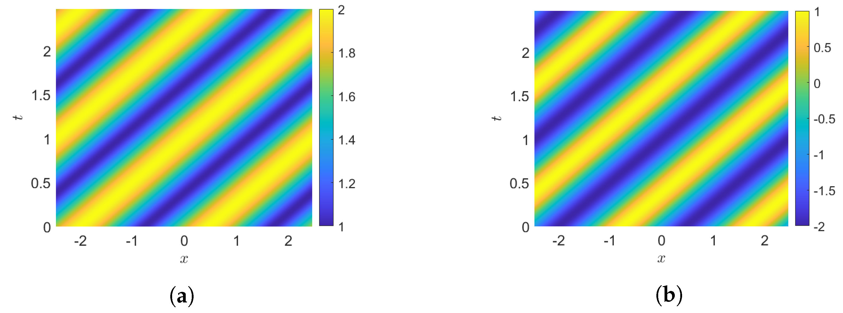
Figure 2.
Delta amplitude solution with , , , , , , . (a). Short wave . (b). Long wave L.
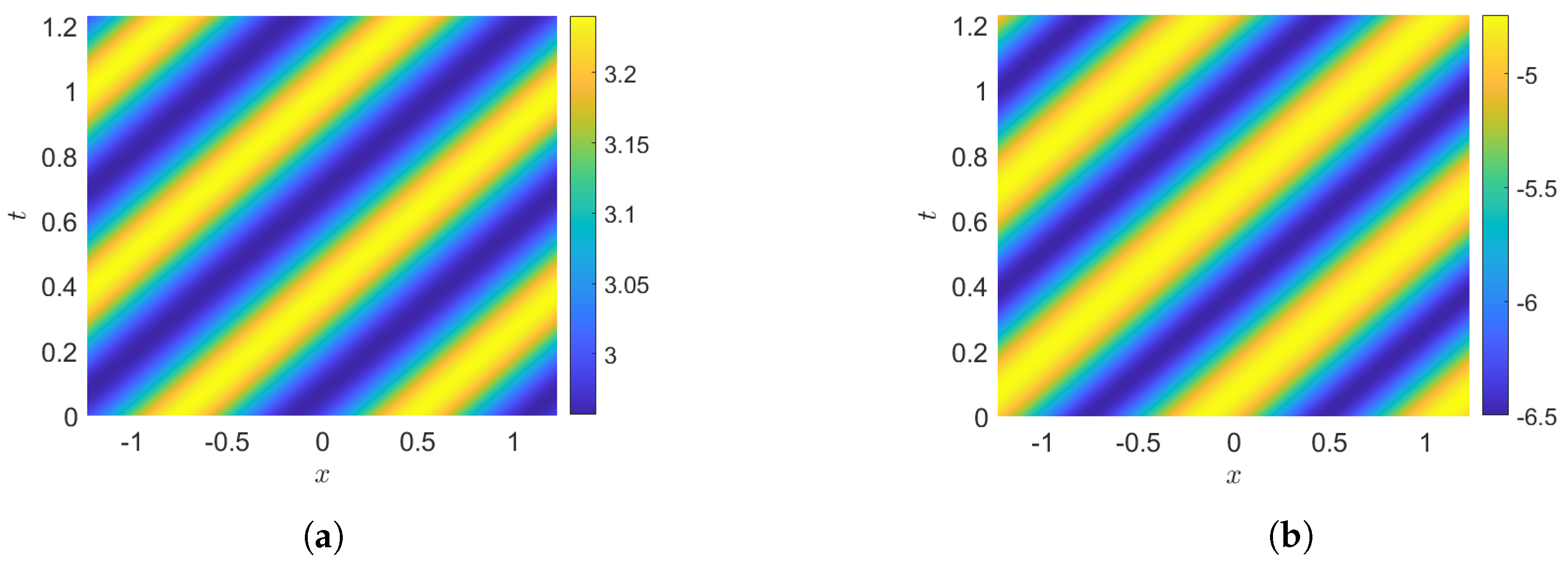
Figure 3.
Bright soliton solution, with , , , , , . (a). Short wave . (b). Long wave L.
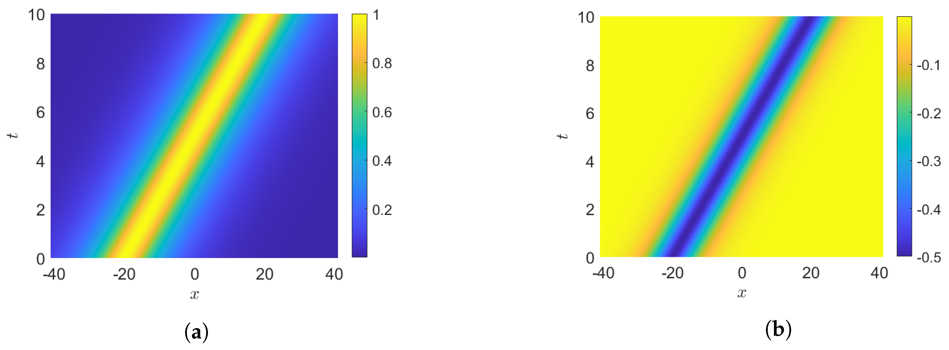
Figure 4.
Rational solution with , , . (a). Short wave . (b). Long wave L.

Publisher’s Note: MDPI stays neutral with regard to jurisdictional claims in published maps and institutional affiliations. |
© 2022 by the authors. Licensee MDPI, Basel, Switzerland. This article is an open access article distributed under the terms and conditions of the Creative Commons Attribution (CC BY) license (https://creativecommons.org/licenses/by/4.0/).
Share and Cite
MDPI and ACS Style
Caso-Huerta, M.; Degasperis, A.; Leal da Silva, P.; Lombardo, S.; Sommacal, M. Periodic and Solitary Wave Solutions of the Long Wave–Short Wave Yajima–Oikawa–Newell Model. Fluids 2022, 7, 227. https://doi.org/10.3390/fluids7070227
AMA Style
Caso-Huerta M, Degasperis A, Leal da Silva P, Lombardo S, Sommacal M. Periodic and Solitary Wave Solutions of the Long Wave–Short Wave Yajima–Oikawa–Newell Model. Fluids. 2022; 7(7):227. https://doi.org/10.3390/fluids7070227
Chicago/Turabian StyleCaso-Huerta, Marcos, Antonio Degasperis, Priscila Leal da Silva, Sara Lombardo, and Matteo Sommacal. 2022. "Periodic and Solitary Wave Solutions of the Long Wave–Short Wave Yajima–Oikawa–Newell Model" Fluids 7, no. 7: 227. https://doi.org/10.3390/fluids7070227