The Influence of Characteristic Sea State Parameters on the Accuracy of Irregular Wave Field Simulations of Different Complexity

Abstract

The accurate description of the complex genesis and evolution of ocean waves, as well as the associated kinematics and dynamics is indispensable for the design of offshore structures and the assessment of marine operations. In the majority of cases, the water-wave problem is reduced to potential flow theory on a somehow simplified level. However, the nonlinear terms in the surface boundary conditions and the fact that they must be fulfilled on the unknown water surface make the boundary value problem considerably complex. Hereby, the contrary objectives with respect to a very accurate representation of reality and numerical efficiency must be balanced wisely. This paper investigates the influence of characteristic sea state parameters on the accuracy of irregular wave field simulations of different complexity. For this purpose, the high-order spectral method was applied and the underlying Taylor series expansion was truncated at different orders so that numerical simulations of different complexity can be investigated. It is shown that, for specific characteristic sea state parameters, the boundary value problem can be significantly reduced while providing sufficient accuracy.

1. Introduction

The design of offshore structures, as well as the assessment of marine operations require an accurate description of the expected surface wave loads, ensuring efficient and safe operations. Thus, precise knowledge of the genesis and evolution of waves through their corresponding kinematics and dynamics is indispensable. To this end, a sound understanding of irregular sea state simulations is critical, because the physical mechanisms of ocean waves embed a relatively large range of different phenomena (i.e., resonant and non-resonant wave–wave interaction effects with different characteristic scales). To describe the relevant physics, various theories and numerical methods have been developed. Since the numerical complexity of wave models increases with their accuracy, computational efficiency and accuracy must be weighed according to the requirements of the investigated problem. One illustrative example is the deterministic wave prediction, for which computations have to be performed faster than in real time while allowing the model to represent all the phenomena that are likely to influence the kinematics and dynamics of the considered wave field within the prediction horizon. In most cases, the water-wave problem is reduced to the potential flow theory; see [1] for a historical overview.

The development of established wave theories is based on extensive studies of Stokes [2]. The Cauchy problem is approximated in Stokes wave theory by applying the perturbation method and linking the perturbation parameter to the wave steepness. The first-order solution of the Stokes expansion is referred to as the linear wave theory, which is also known as the Airy wave theory [3]. Higher-order solutions are obtained by higher-order expansions of the velocity potential and the surface elevation. These solutions include nonlinearities such as a crest–trough asymmetry and an increase in the wave propagation speed due to wave steepness (e.g., [4,5]).

Linear wave theory is a rather simple and fast approach that is capable of providing acceptable results for many different ocean engineering applications. Thus, the linear approach is widely used and serves as a standard model for ocean waves. The theoretical foundation is based on the linear superposition of independent wave components, each having a different frequency and amplitude (and direction of propagation in the case of directional wave fields). In addition, the propagation velocity of the component waves depends only on the wave frequency and the water depth. As a consequence, supposing a constant water depth and with the knowledge of its energy density spectrum, the wave field can be estimated at any time/location of interest by shifting the wave components.

Based on wind–wave generation processes characterizing the energy transfer between the wind blowing over the sea surface and surface waves, the growth of the wave heights can be predicted in the form of an energy distribution along the wave frequencies of the wave field. Taking into account the strength of the wind (generally represented by the wind speed in the atmospheric boundary layer) and characteristic space and time scales over which the wind is blowing, standard wave spectra have been introduced (e.g., [6,7,8]). Among them, the empirical Pierson–Moskowitz spectrum [8] gives the shape of a wave spectrum for a fully developed sea state, i.e., the wind is steadily blowing over a large area and over a long time, as a function of the wind speed at 10 m above the sea surface (which can be directly related to the total energy of the wave field) and the frequency of maximal energy, referred to as the peak frequency. This spectral shape was later adapted to young (or non-fully developed) sea states, for which the spectral shape exhibits a narrower energy distribution around the peak frequency. The level of development of the sea state has been investigated during the Joint North Sea Wave Project [9], leading to the well-known JONSWAP spectrum. This spectrum uses a peak enhancement factor that represents the influence of the propagation time of the wave field on the spectral shape. These spectra are essential for design purposes and serve as standardized design wave spectra in many areas of application, such as the study of wave characteristics, wave statistics, wave generation, and stochastic, as well as deterministic wave–structure interaction. Assuming linear motion behavior, in addition to the wave linearity, the spectral perspective of wave–structure interaction offers many options for evaluating offshore structures (e.g., [10,11,12,13]).

However, simplifications of the water-wave problem pertaining to the linear approach imply uncertainties. As nonlinear effects become important with increasing wave steepness, the accuracy of the linear solution decreases significantly. Alternatively, more advanced nonlinear methods can be utilized. In this context, the nonlinear potential flow theory is suitable for simulating the majority of relevant nonlinear wave effects. Nevertheless, the practical applicability of nonlinear potential flow solvers is limited to non-breaking conditions due to their inability to model extreme wave heights and wave breaking physically, i.e., only approximated solutions are available to account for the energy dissipation and to avoid numerical instabilities (e.g., [14,15]). However, there is a variety of different nonlinear potential flow theory methods of different orders of complexity available—from weakly nonlinear models to fully nonlinear simulations. Generally, the computational effort increases with increasing complexity, i.e., the high accuracy of fully nonlinear numerical methods comes at the expense of high computational costs, and the resulting solutions are usually expressed on a discretized finite spatio-temporal domain, requiring extra work to post-process the results compared to the reduced-order and linear wave theories. A review of nonlinear free surface flow simulation techniques can be found in Westhuis [16] and in the references therein.

Among them, the envelope equations of the nonlinear Schrödinger equation (NLSE) framework capture weakly nonlinear effects in a numerically efficient way [17,18,19,20,21]. Under the assumption of small-amplitude waves and a narrow-banded wave spectrum centered around a characteristic carrier wavelength, the description of the surface evolution is determined by means of modulations of the carrier wave. Both the NLSE and the modified NLSE (MNLSE)—which includes higher-order terms—have been investigated extensively, experimentally and numerically, in terms of nonlinear wave evolution (e.g., [21,22,23,24,25,26]). Although the NLSE captures relevant nonlinear phenomena and shows good accuracy for sufficiently narrow spectra, it has been generally shown that, due to the spectral bandwidth constraint, it is less suitable for simulating broader-band irregular sea states [27]. However, the MNLSE, together with a modeling of the full dispersive effects, provides significantly better results (e.g., [20,24,27]).

Another notable nonlinear method used frequently for wave simulation is the numerically efficient High-Order Spectral (HOS) method [28,29]. This pseudo-spectral approach solves the water-wave boundary value problem up to any arbitrary order of nonlinearity. Because the majority of the calculations are performed in the Fourier space (usually using a fast Fourier transform), the HOS method exhibits a high computational efficiency. Numerous studies have shown the suitability of the HOS approach for a wide range of applications: the simulation of long-term and large-scale wave fields for freak wave analysis [30,31], the modeling of a numerical wave tank [32], and the prediction of nonlinear wave fields from wave measurements [27,33,34,35,36] are only a few examples illustrating its versatility.

The HOS method has been applied for intensive investigations on the general applicability and limitations of highly nonlinear potential flow solvers [37]. Thereby, the focus has been on the limit of the non-breaking wave condition and on the characteristic sea state parameters that violate this condition. For this purpose, the JONSWAP spectrum has been applied for the generation of the initial wave fields, and the influence of discretization, water depth, directional spreading, spectral peakedness, and significant wave height has been studied. To overcome the identified limitations, methods to localize breaking events and to model the associated energy dissipation have been introduced for the HOS method, proving to be effective (e.g., [14,15]). Consequently, the HOS method can be seen as a mature approach for ocean engineering applications, which motivates the choice of this model for the study presented in this paper.

Considering the HOS method as a ”good example of nonlinear potential flow solvers” [37], this method is predestined for answering the question about the necessary model accuracy for certain characteristic sea state parameters since different orders of complexity can be straightforwardly taken into account without any influence on the basic theoretical foundation. On the one hand, such a systematic investigation aims to provide a better understanding of the capabilities of nonlinear models of different complexity. On the other hand, it will help to limit the computational effort of the HOS method to its minimal requirement, thus facilitating use in ocean engineering applications.

For this study, the impact of the different levels of modeling complexity (i.e., HOS of nonlinearity) was systematically evaluated for different characteristic sea state parameters, namely the spectral peak enhancement factor of the JONSWAP wave spectrum, the directional spreading, the wave steepness, and the propagation time. The fourth-order ($\mathrm{M}=4$) solution of the HOS method serves as a reference taking all resonant and non-resonant effects up to five-wave interactions into account.

The paper is organized as follows. Section 2 presents the theoretical foundation of this study, starting with the general overview of the potential flow theory and boundary value problem, then detailing the implementation of the HOS method. Section 3 describes the numerical setup and parameters whose influences on the accuracy of HOS simulations of different orders were investigated. The corresponding numerical results are presented in Section 4. A semi-experimental approach, based on wave probe data measured in a physical wave tank and corresponding simulations from its digital twin, is presented in Section 5 for the validation of the numerical results. The conclusions are drawn in Section 6.

2. Theoretical Foundation

Under the assumption that the Newtonian fluid is incompressible, inviscid, and irrotational, its velocity potential $\varphi$ satisfies the Laplace equation:

$$\frac{{\partial }^2\varphi }{\partial x^2}+\frac{{\partial }^2\varphi }{\partial y^2}+\frac{{\partial }^2\varphi }{\partial z^2}=0.$$

(1)

The sea bottom and the unknown free surface represent the boundaries of the fluid domain. Assuming that the sea bottom is level, rigid, and impermeable at $z=-d$, the normal component of the flow velocity disappears:

$$\frac{\partial \varphi }{\partial z}=0\mathrm{on} z=-d.$$

(2)

The kinematic boundary condition at the free surface describes that no particle leaves the free surface:

$$\frac{\partial \zeta }{\partial t}+\frac{\partial \varphi }{\partial x}\frac{\partial \zeta }{\partial x}+\frac{\partial \varphi }{\partial y}\frac{\partial \zeta }{\partial y}-\frac{\partial \varphi }{\partial z}=0\mathrm{on} z=\zeta (x,y,t).$$

(3)

The dynamic boundary condition defines that the dynamic pressure at the free surface is constant and equal to the atmospheric pressure:

$$\frac{\partial \varphi }{\partial t}+\frac{1}{2}\left({\left(\frac{\partial \varphi }{\partial x}\right)}^2+{\left(\frac{\partial \varphi }{\partial y}\right)}^2+{\left(\frac{\partial \varphi }{\partial z}\right)}^2\right)+g\zeta =0\mathrm{on} z=\zeta (x,y,t).$$

(4)

Both kinematic and dynamic boundary conditions must be fulfilled at the unknown free surface $z=\zeta (x,y,t)$, resulting in a complex boundary value problem.

High-Order Spectral Method

The HOS method was independently introduced by West et al. [28] and Dommermuth and Yue [29]. This numerical method is based on the Zakharov equation [17] and the comparable mode-coupling approaches [38,39] and allows capturing a high number of free wave modes. To solve the nonlinear initial boundary value problem, the Taylor series of arbitrary nonlinear order is applied to expand the mean water level quantities to the free surface. The use of global basis functions together with the identity of the vertical derivatives with the surface Laplacian essentially allows using the fast Fourier transform for this pseudo-spectral approach and solving the nonlinear wave dynamics very efficiently [28,29,40]. This method takes, up to a given order, all nonlinear interactions, resonant and non-resonant, into account and can be applied for long- and short-crested sea states. Additionally, wave–current, as well as wave–bottom interactions can be considered.

For this paper, the numerical procedure presented in West et al. [28] was used. Implementing this pseudo-spectral method, all derivatives related to the potential and surface elevation are determined in the Fourier space assuming periodic conditions on the vertical domain boundaries, whereas nonlinear products are calculated in the physical space. At the beginning, the potential equations are converted to equations at the free surface $\Psi (\mathit{x},t)\equiv \varphi (\mathit{x},\zeta ,t)$, with $\mathit{x}={[x,y]}^{⊺}$. Applying chain rules, the kinematic boundary condition at the free surface (Equation (3)) can be rewritten as

$$\frac{\partial \zeta }{\partial t}=-▿\Psi ·▿\zeta +W(1+{\left|▿\zeta \right|}^2)\mathrm{on} z=\zeta .$$

(5)

The dynamic boundary condition reads:

$$\frac{\partial \Psi }{\partial t}=-g\zeta -\frac{1}{2}{\left|▿\Psi \right|}^2+\frac{1}{2}{W}^2(1+{\left|▿\zeta \right|}^2)\mathrm{on} z=\zeta ,$$

(6)

with ${W=\partial \varphi /\partial z|}_{z=\zeta }$ as the vertical velocity at the free surface and $▿=\partial /\partial \mathit{x}$ as horizontal gradient operator.

By using Equations (5) and (6) as free surface boundary conditions, the boundary value problem is now exclusively related to the vertical velocity W, which can be determined in terms of $\zeta$ and $\Psi$ by series expansion. The procedure by West et al. [28] starts from the formal expression that the surface velocity potential $\Psi$ can be represented as the Taylor series expansion at $z=0$ and yields

$$\Psi (\mathit{x},t)=\sum _n{\left.\frac{{\zeta }^n}{n!}\frac{{\partial }^n\varphi }{\partial z^n}\right|}_{z=0}.$$

(7)

Accordingly, the vertical velocity W is obtained by

$$W(\mathit{x},t)=\sum _n{\left.\frac{{\zeta }^n}{n!}\frac{{\partial }^{n+1}\varphi }{\partial z^{n+1}}\right|}_{z=0}.$$

(8)

Now, the problem is transformed into the reference function $\varphi$ in order to be solved for the boundary value problem at $z=0$. Assuming that $\Psi$ and $\zeta$ are quantities of $\mathcal{O}\left({\zeta }^n\right)$, $\varphi$ and W are expanded by perturbation series according to

$$\begin{array}{cc}\hfill \varphi (\mathit{x},z,t)& =\sum _{n=0}^m{\varphi }^{\left(n\right)}(\mathit{x},z,t),\hfill \end{array}$$

(9)

$$\begin{array}{cc}\hfill W(\mathit{x},t)& =\sum _{n=0}^m{W}^{\left(n\right)}(\mathit{x},t),\hfill \end{array}$$

(10)

with $\zeta$ as the ordering parameter and $\mathrm{M}=m+1$ being the order of approximation of nonlinearity. Using Equation (7), separating the terms of each order $\mathcal{O}\left({\zeta }^n\right)$ gives

$${\varphi }^{\left(0\right)}(\mathit{x},0,t)=\Psi (\mathit{x},t)$$

(11)

for the first order. The next higher-order solutions are obtained from the lower-order solutions as

$${\varphi }^{\left(m\right)}(\mathit{x},0,t)=-\sum _{n=1}^m{\left.\frac{{\zeta }^n}{n!}\frac{{\partial }^n{\varphi }^{(m-n)}}{\partial z^n}\right|}_{z=0}.$$

(12)

The vertical velocity W at the surface $\zeta$ is obtained by

$$W^{\left(m\right)}(\mathit{x},t)=\sum _{n=0}^m{\left.\frac{{\zeta }^n}{n!}\frac{{\partial }^{n+1}{\varphi }^{(m-n)}}{\partial z^{n+1}}\right|}_{z=0}.$$

(13)

Furthermore, the physical quantities $\varphi$, $\Psi$, and $\zeta$ are expressed by means of basis functions that satisfy Equations (1) and (2). Assuming periodic conditions on the horizontal boundaries of the computational domain, basis functions such as the velocity potential can be derived in the Fourier space by

$$\varphi (\mathit{x},z,t)=\frac{1}{2\pi }\underset{-\infty }{\overset{\infty }{\int }}\widehat{\varphi }(\mathit{k},t)\frac{cosh\left(\left|\mathit{k}\right|(z+d)\right)}{cosh\left(\left|\mathit{k}\right|d\right)}{e}^{\mathrm{i}\mathit{k}·\mathit{x}}\mathrm{d}\mathit{k},$$

(14)

with $\widehat{\varphi }(\mathit{k},t)$ as Fourier coefficients and $\mathit{k}$ denotes the wave number vector with $\mathit{k}={\left[\begin{array}{c}{k}_x,k_y\end{array}\right]}^{⊺}$ for two-dimensional spatial inputs. Similar expressions without the z-dependency are used for $\Psi$ and $\zeta$. This formulation allows using a fast Fourier transform algorithm, leading to very efficient computations of the spatial derivatives of the physical quantities. This results in “(near) linear computational effort”, as well as “exponential convergence (…) being notable characteristics of the computational efficacy of HOS methods” [40].

Generally, the HOS method can be utilized to any order of nonlinearity $\mathrm{M}$ due to the recursive approach for the calculation of the higher-order terms (Equations (12) and (13)). Practically, the HOS order is limited due to aliasing effects, as well as numerical errors and instabilities resulting in high-frequency contamination in the Fourier space [28,40,41]. The nonlinear products of the pseudo-spectral approach are performed in the physical space domain, which is represented by Fourier modes at equally spaced points, resulting in aliasing errors that become more and more significant with increasing order [28,40]. The aliasing effect limits the finite Fourier space that can be taken into account for the simulation. This problem can theoretically be avoided by increasing the number of Fourier modes with increasing order, i.e., increasing the number of discrete space points by decreasing the discrete step size $\Delta x$ in the physical space domain [28]. However, computational resources and aspects of numerical efficiency limit this approach significantly, particularly for $2D+1$ simulations.

The numerical error can be quantified in terms of the error in the spectral representation, as well as truncation error. The numerical error for the spectral representation vanishes exponentially as the number of component waves goes to infinity [40]. Furthermore, the truncation error vanishes exponentially with increasing $\mathrm{M}$ for mild nonlinearities [40]. The convergence is theoretically limited to the maximum wave steepness of the free surface, but practically, the convergence characteristics end at certain wave steepness before the maximum wave steepness is reached [40]. In addition, Nicholls and Reitich discussed the stability of high-order perturbative methods for the computation of Dirichlet–Neumann Operators (DNOs), showing that “the convergence of these algorithms is, quite generally, limited by numerical instability (…)” and that “these standard perturbative methods for the calculation of DNO suffer from significant ill-conditioning which is manifest even for very smooth boundaries, and whose severity increases with boundary roughness” [41]. Consequently, in most applications, the HOS method is limited in terms of nonlinearity order ($\mathrm{M}\le 5$), finite Fourier space (in terms of multiples of peak wave period), and maximum initial wave (spectrum) steepness [37] due to these numerical limitations and constraints.

For this study, a low-pass filter was implemented to avoid Fourier space aliasing for higher-order terms [28]. Additionally, an exponential damping term was introduced in the Fourier space to suppress high-frequency contamination that can occur for the highest waves, causing numerical instabilities. To do so, the Fourier coefficients of ${\zeta }_t$ and ${\Psi }_t$ were damped at a specific wave number $k_{damp}$ after each time step by an exponential term, which reaches zero at $k_{end}$. The specific wave number was set to $k_{damp}=6k_p$ and $k_{end}=1.3k_{damp}$ for this study after systematic investigations of different wave steepness, with $k_p$ as the peak wave number of the considered sea states. This value showed no influence on lower wave steepness, but stabilized the simulations with the highest wave steepness. However, the procedure was neither capable of handling wave-breaking effects, nor simulating steep waves close to breaking: the simulated wave fields presented hereafter all fall into the applicability domain of nonlinear potential flow solvers, as described in [37]. In this study, the fourth-order Runge–Kutta–Gill method was applied to advance the evolution equations in time.

3. Numerical Setup and Program

The following study comprises investigations of irregular sea states based on the JONSWAP spectrum, evaluating the influence of wave steepness, peak enhancement factor, directional spreading factor, and simulation time on the accuracy of the wave simulations of different complexity.

Different complexity denotes that each of the investigated sea states was simulated at four different orders of the HOS approach, from the first to the fourth order. The solutions of the different orders are hereinafter referred to as HOSMX with X labeling the respective Xth-order solution. First, the investigations were carried out using the fourth-order simulation as a reference and comparing the lower-order simulations to this reference simulation. The numerical setup and parameters were identical for all simulations. The size of the quadratic domain was chosen to be $x=y=2000$ m with a water depth of $d=5000$ m. The domain was discretized by $N_x=N_y=2^{10}$ grid points, resulting in a spatial resolution of $\Delta x=\Delta y\approx 1.95$ m. The simulation time was set to $t_{sim}=250$ s with a temporal resolution of $\Delta t=0.05$ s. For the evaluation of the simulation results, surface elevation snapshots of the respective simulations were stored at every 2000 time steps ($t_{snapshot}=10$ s) for subsequent post-processing.

To evaluate the results quantitatively, the surface similarity parameter ($\mathrm{SSP}$) [42] was used to compare the surface elevation snapshots of the different orders with the reference solution (HOSM4). The $\mathrm{SSP}$ was chosen as this parameter takes the amplitude, as well as the phase difference of two signals or surfaces $f_1$ and $f_2$ into account to quantify the surface similarity. This normalized error ranges between 0 (perfect agreement) and 1 (perfect disagreement) and is calculated as

$$\mathrm{SSP}(f_1,f_2)=\frac{{(\int |F_1\left(\mathit{k}\right)-F_2\left(\mathit{k}\right){|}^2\mathrm{d}\mathit{k})}^{\frac{1}{2}}}{(\int |F_1{\left(\mathit{k}\right)|}^2{\mathrm{d}\mathit{k})}^{\frac{1}{2}}+(\int |F_2{\left(\mathit{k}\right)|}^2{\mathrm{d}\mathit{k})}^{\frac{1}{2}}},$$

(15)

with $F\left(\mathit{k}\right)$ representing the Fourier transform of the signals. The $L^2$-norm of the individual signals $\left|\right|f_i{\left|\right|}^2=\int |F_i\left(\mathit{k}\right){|}^2\mathrm{d}\mathit{k}$ and their respective $L^2$-error in space domain $\left|\right|f_1-f_2{\left|\right|}^2=\int |F_1\left(\mathit{k}\right)-F_2\left(\mathit{k}\right){|}^2\mathrm{d}\mathit{k}$ depicts the basis of the $\mathrm{SSP}$. Consequently, $\mathrm{SSP}$ is calculated in the complex Fourier space and inherently penalizes amplitude-, frequency-, and phase-errors at the same time and in a single quantity. If both signals are identical, the $L^2$-error is 0, such that $\mathrm{SSP}=0$ denotes perfect agreement among the signals/surfaces. Based on previous investigations, the accuracy may be assumed to be acceptable for $\mathrm{SSP}$ values below $0.1$. Figure 1 presents a comparison of two signals to give a picture of the correlation between two signals featuring a $\mathrm{SSP}\approx 0.1$.

As previously mentioned, the JONSWAP spectrum [9] was used to generate the initial wave field in the space domain:

$$S_J\left(\omega \right)=\frac{\alpha g^2}{{\omega }^5}·exp\left[-\frac{5}{4}·{\left(\frac{{\omega }_p}{\omega }\right)}^4\right]·{\gamma }^{exp\left[-\frac{{\left(\omega -{\omega }_p\right)}^2}{2r^2{\omega }_p^2}\right]},$$

(16)

with ${\omega }_p$ the peak wave angular frequency, g the gravitational acceleration, $\alpha$ the Phillips coefficient, $\gamma$ the peak enhancement factor, and r defines the shape of the spectrum on the left- and right-hand side of the peak ($r=0.07$ for $\omega <{\omega }_p$ and $r=0.09$ for $\omega \ge {\omega }_p$). In order to initialize the three-dimensional wave field, the directional spreading function [43]:

$$D(\omega ,\Theta )=\frac{\Gamma \left(\frac{s}{2}+1\right)}{\Gamma \left(\frac{s}{2}+0.5\right)\sqrt{\pi }}·{cos}^s(\Theta ),$$

(17)

was applied to convert the JONSWAP spectrum into a directional spectrum. $\Gamma$ represents the Gamma function, and s is the spreading exponent [43]. To ensure that the energy content of the wave spectrum remains the same, the following equation must be satisfied:

$${\int }_{-\pi }^{\pi }D(\omega ,\Theta )\mathrm{d}\Theta =1.$$

(18)

Consequently, the directional JONSWAP spectrum can be derived by

$$S_J(\omega ,\Theta )=S_J\left(\omega \right)·D(\omega ,\Theta ).$$

(19)

The wave direction was defined for $\Theta \in [-\frac{\pi }{2},\frac{\pi }{2}]$ with a discrete directional angular increment of $\Delta \Theta =\pi /24$.

The JONSWAP spectrum was applied to generate a set of irregular sea states with a peak period of $T_p=10$ s and systematically varied wave steepness $ϵ=k_p{H}_s/2$; enhancement factor $\gamma$. $H_s$ represents the significant wave height, and the wavelength and the wave period are linked via the linear dispersion relation $\omega =\sqrt{gktanhkd}$. Note that this relationship between k and $\omega$ is only assumed for the definition of the initial surface elevation snapshot; the wave field evolution is performed according to the HOS equations at the considered order of nonlinearity without further assumption.

Table 1. Overview of the numerically investigated characteristic sea state parameters.

Sea State	${\mathit{T}}_{\mathit{p}}$	${\mathit{H}}_{\mathit{s}}$ ($\mathit{ϵ}$)	$\mathit{\gamma }$
1	10 s	1.24 m (0.025)	1
2			3
3			6
4		1.86 m (0.0375)	1
5			3
6			6
7		2.48 m (0.05)	1
8			3
9			6
10		3.73 m (0.075)	1
11			3
12			6
13		4.97 m (0.1)	1
14			3
15			6
16		6.21 m (0.125)	1
17			3
18			6

shows the selected sea states. The simulations were carried out for six wave steepnesses ($0.025\le ϵ\le 0.125$) representing small, moderate, and steep waves and three different peak enhancement factors. Besides this, the spreading factor was additionally varied in order to investigate a possible influence of the directionality on the different HOS orders. For this purpose, the initial spatial wave field was calculated for spreading factors of $s=[300,30,4]$ representing sea states from almost long- to short-crested wave distributions. In addition, a fully long-crested wave field ($\Theta =0$) was also initialized, i.e., constant wave height in the y-direction, to cover the classical 2D application and to put it into relation with the directional wave field simulations.

Consequently, 72 different parameter combinations were used for the determination of the initial wave fields. Hereby, it must be noted that this only applies to the wave spectrum as the phase distribution was only generated once randomly and afterwards used for all sea state realizations. Thus, an influence of the phase distribution on the simulation results of the different parameter combinations and HOS orders can be excluded, i.e., the difference can be directly related to the different input parameters. The initialized wave fields were used to simulate the wave propagation for the four different HOS orders, and the HOSM4 served as a reference solution to evaluate the lower orders.

4. Numerical Results

Figure 2 presents the results of the investigated sea states shown in Table 1. Each diagram shows the SSP of the three lower orders HOSM1 (blue curves), HOSM2 (red curves), and HOSM3 (green curves) over time, where HOSM4 served as the reference solution. Each diagram shows the SSP of the investigated sea states with varying directionality: long-crested waves (solid lines) and short-crested waves with spreading factors of 300 (dashed lines), 30 (dashed-dotted lines), and 4 (dotted lines). For a better overview, the curves are displayed with slightly varying colors. The rows depict sea states with constant wave steepness and increasing enhancement factor from left to right. For sea states in one column, the enhancement factor is kept constant and the wave steepness increases from top to bottom. For a better comparison, the y-axis has a limit of 0.4. The curves that were cut off show an approximately linear increase. As previously mentioned, the accuracy is assumed to be acceptable in the following discussion for SSP values below $0.1$ (cf. Figure 1).

It can be seen that for sea states with a small wave steepness of $ϵ\le 0.0375$, the accuracy of HOSM3, HOSM2, and HOSM1 remains high over the total simulation time of $t_{sim}=250$ s. This is due to the low impact of nonlinear effects for small wave steepness. With increasing nonlinear effects for increasing wave steepness, the accuracy of HOSM1 and HOSM2 decreases significantly. In this context, the first-order solution ($\mathrm{M}=1$) of the HOS method is equivalent to linear wave theory in terms of wave–wave interaction and the dispersion of waves. For the second-order solution ($\mathrm{M}=2$), quadratic nonlinear effects (three-wave interaction) are taken into account, which results in a better performance with increasing wave steepness, which is clearly evident when considering the increasing discrepancy between the first- and second-order simulation results with increasing steepness. Consequently, the application area for the first- and second-order solutions is limited to small wave steepness. With increasing steepness, the application area in terms of accuracy over simulation time decreases fast to only five peak periods or less for $ϵ\ge 0.075$ with HOSM1 and for $ϵ\ge 0.1$ with HOSM2. Nevertheless, this low level of complexity (i.e., high numerical efficiency) may still be relevant for very short-term predictions, i.e., in terms of forecast distance and horizon, such as needed for the control of marine energy devices such as wave energy converters or floating offshore wind turbines.

The HOSM3 simulations show significantly better accuracy for all investigated wave steepnesses. The reason for this lies in the fact that the step from second to third order denotes significant improvements from a physical point of view. For $\mathrm{M}=3$, cubic nonlinear effects (four-wave interaction including modulational instability) yielding nonlinear corrections of the dispersion relation are taken into account. The discrepancy to the reference solution (HOSM4-quartic nonlinear effects) even for the highest investigated steepness shows that the relevant physics is already captured by HOSM3. However, it can be expected that the discrepancy increases for steeper sea states, i.e., the fourth-order solution of the HOS method may be the right choice for steeper sea states having in mind the aforementioned limitations regarding wave breaking, numerical efficiency, and instabilities.

Evaluating the influence of the peak enhancement factor reveals a strong influence on the accuracy of the simulation as with increasing $\gamma$, the accuracy increases for the same steepness and all investigated orders of the HOS method. This effect is more pronounced for the first- and second-order solutions, as well as increasing wave steepness. Detailed investigation on this question could not conclusively clarify the reasons for this, but a reasonable explanation may be that the wider energy distribution for smaller enhancement factors triggers more nonlinear dynamics in terms of wave–wave interaction, as well as the dispersion of waves: there are more short waves riding long waves, leading to a higher number of local steep events (i.e., high slope) and locally triggering nonlinear physical phenomena. On the other hand, this explanation may contradict the identified influence of the large Benjamin–Feir Index (BFI) on nonlinear wave propagation processes, e.g., [44], which is related to large wave steepness and narrow bandwidth spectra (i.e., high enhancement factor). Thus, additional investigations need to be addressed to this question. In this context, it is interesting to see in Figure 2 that the directional spreading factor has nearly no effect on the accuracy of the simulation.

So far, the numerical results show that for the same sea state, i.e., in terms of the phase distribution of the initial wave field, the wave steepness, in particular, plays a major role in terms of the accuracy of the different orders. However, the question of the influence of the random phase distribution is still unanswered: Are the differences identified in Figure 2 generally valid and thus independent of the initial phase distribution, or do the results only represent a specific individual case (i.e., other initial phase distributions yield significantly different results)?

To investigate whether the initial phase distribution has a significant influence, simulations with 30 different random phase distributions were performed for one sea state ($T_p=10$ s, $ϵ=0.075$, $\gamma =6$, $s=4$). Figure 3 shows the mean value of the $\mathrm{SSP}$ for all 30 simulations for HOSM1 (blue curve), HOSM2 (red curve), and HOSM3 (green curve). The Standard Deviation (SD) is shown as a transparent area of the same color. It can be seen that $\mathrm{SSP}$ does not vary much for the different phase distributions. Therefore, it can be concluded that the results obtained are generally valid.

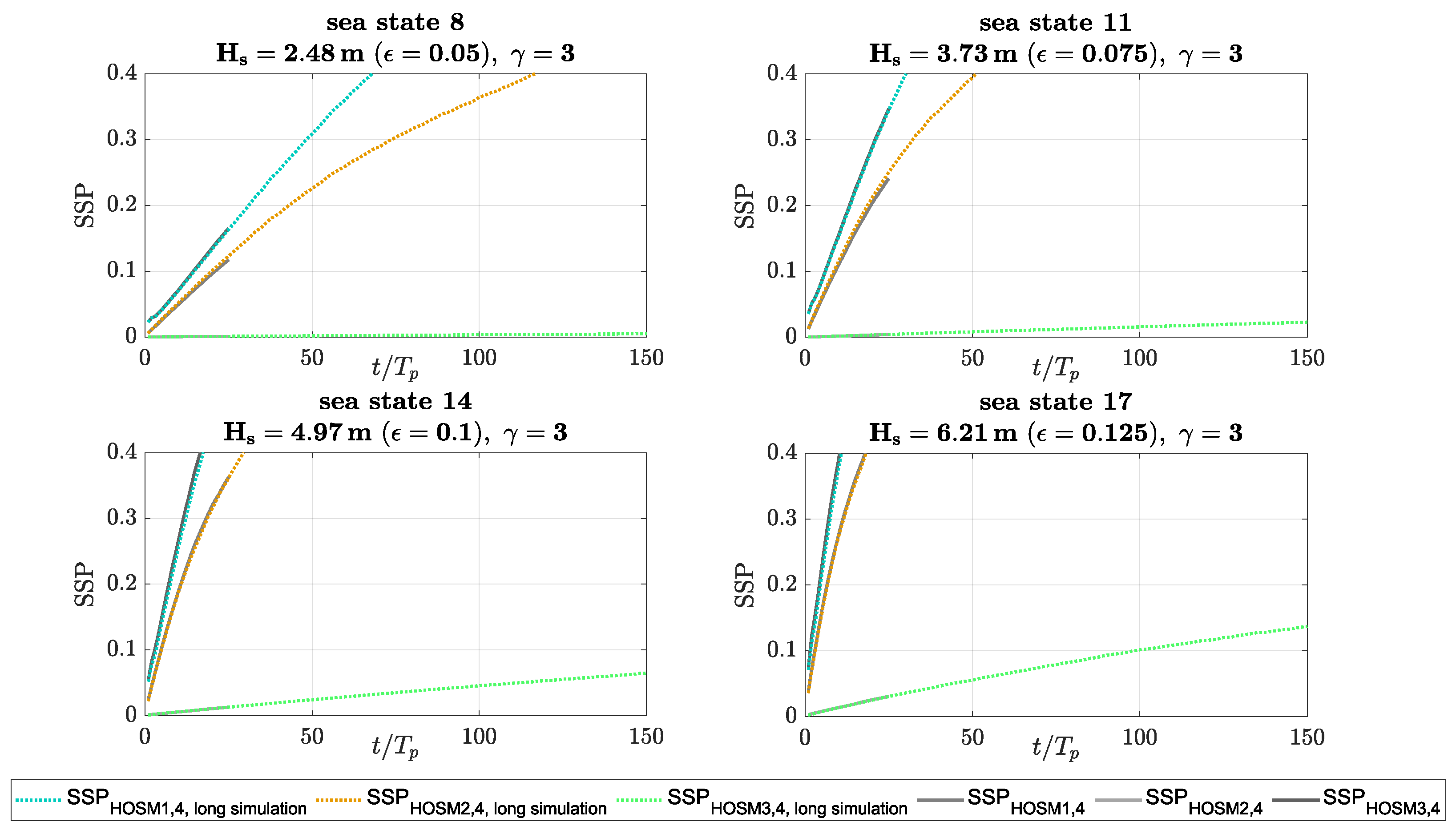
Finally, long-term simulations were performed in order to evaluate if a simulation time of $t_{sim}=25T_p$ provides a sufficient conclusion about the applicability of the different orders or if longer simulation times yield significantly different results due to the nonlinear effects of a larger time scale. For this purpose, long-term simulations ($t_{sim}=150T_p$) were performed for selected sea states. Hereby, the spreading factor ($s=4$) and enhancement factor ($\gamma =3$) were kept constant, whereas the four largest wave steepnesses were selected. In addition, all orders of nonlinearity were investigated.

Figure 4 presents the results for the selected sea states. Again, the results for HOSM1 are shown as a blue dotted line, for HOSM2 as a red dotted line, and for HOSM3 as a green dotted line. In addition, the respective results shown in Figure 2 are illustrated for comparison as grey lines. The results show that the course of $\mathrm{SSP}$ does not change significantly at later simulation times. Generally, the course of $\mathrm{SSP}$ follows a somewhat linear rate of increase for all sea states. Later on, at higher absolute SSP values, this linear rate of increase tends to reach an asymptotic horizontal course for very large $\mathrm{SSP}$ values ($\mathrm{SSP}\ge 0.7$). This asymptotic behavior does not correspond to any physical mechanism within the simulations nor simulation time, and the reason lies solely in the way in which the $\mathrm{SSP}$ is calculated (“perfect disagreement” results in a $\mathrm{SSP}=1$). However, for this study, $\mathrm{SSP}$ values above $\mathrm{SSP}\ge 0.2$ already represent an unacceptable inaccuracy, which is below the $\mathrm{SSP}$ values at which the asymptotic behavior starts. Thus, the curves in Figure 4 show that the results of the short-term simulations are confirmed by the long-term simulations, i.e., a linear rate of increase for longer simulation times can be assumed.

5. Experiments

Following, the numerical findings are examined by experiments. For this purpose, experiments on irregular sea states were conducted in a wave tank and the measurement results were compared to the numerical simulations of the different HOS orders. The experiments were carried out in the seakeeping basin of the Ocean Engineering Division at Technische Universität Berlin (TUB). The basin is $110$ m long, $8$ m wide, and $1$ m deep, with a $90$ m measuring range. The long-crested waves are generated by an electrically driven, fully computer-controlled wave generator that can operate in both piston and flap-type mode. The wave generation software enables the generation of regular waves, transient wave packets, and irregular waves. A wave damping slope is installed on the opposite side to suppress disturbing wave reflections.

Table 2. Overview of the experimentally investigated characteristic sea state parameters.

Sea State	${\mathit{T}}_{\mathit{p}}$	${\mathit{H}}_{\mathit{s}}$ ($\mathit{ϵ}$)	$\mathit{\gamma }$
1	8.58 s	1.83 m (0.05)	1
2			3
3			6
4		3.66 m (0.1)	1
5			3
6			6
7		5.48 m (0.15)	1
8			3
9			6

shows the characteristic parameters of the investigated irregular sea states. As with the numerical studies, the basis for the wave generation was the JONSWAP spectrum, and the wave steepness and enhancement factor were varied.

Generally, the experimental validation of the HOS method is almost impossible with classical experimental equipment. In contrast to the HOS approach, which needs the surface elevation in the space domain as the initial condition, the surface elevation is normally measured at a distinct position in space over time during the experiments. Thus, measuring the surface elevation in the space domain would require multiple, continuous point-by-point measurements (with a reasonable calm-down time in between) to obtain a snapshot. To overcome this problem, the experimental validation was performed by using a semi-experimental approach. The semi-experimental approach has been introduced to create input snapshots based on the irregular waves generated during the experiment [27]. The nonlinear numerical wave tank waveTUB [45,46,47] served as a digital twin to determine the input snapshots of the experimentally generated irregular waves. Besides identical main dimensions, the main feature is the capability to model the exact geometry of the wave maker so that the boundary conditions are identical at the wave board, i.e., providing an identical starting point of the wave evolution for both tanks. Thus, in order to generate the input wave snapshots, the physical wave board motion is used to reproduce the irregular sea states in the numerical wave tank waveTUB.

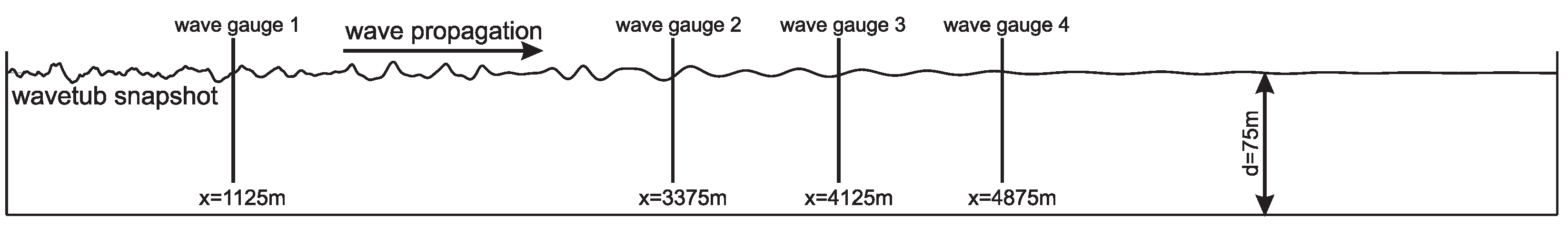
Figure 5 shows a side view of the wave tank (all data in full scale) and the general scheme of the procedure. On the left is the wave maker and on the right a wave-damping beach. A snapshot of the surface elevation at a given point in time is also displayed, indicating the initial condition for the HOS simulations. For the experiments, four wave gauges were installed to validate the waveTUB input snapshots pointwise (wave gauge 1) and to compare the simulation results with the measurements in the time domain at three fixed positions (Wave Gauges 2–4).

The measuring principle of the applied wave gauges is based on surface-piercing resistance-type wires. The surface-piercing wires feature a very small diameter so that the wave system is not affected by the presence of the wave gauge. The advantage of the applied wave gauges over non-contact measurement systems (such as ultrasound or down-looking radar measurement systems) is the fact that very steep waves and wave breaking can be measured very accurately. Altogether, the applied wave gauges represented an established measurement technique that enables accurate detection of the waves. Once accurately calibrated, the wave probes serve a sub-millimeter precision. The calibration process followed a standardized procedure that ensures an accurate setup of the measuring system. Based on this procedure, the overall calibration error is known to be less than $1\%$. Such calibration error denotes that the measured surface elevation features a constant offset in the water column compared to the expected value, i.e., the amplitudes are affected, but not the phases of the signal. In terms of investigated sea states (cf. Table 2), this error affects $\mathrm{SSP}$ theoretically by $\mathrm{SSP}\le \pm 0.01$.

For each reproduced sea state, eight consecutive snapshots ($\Delta t_{snapshot}=43 \mathrm{s}\approx 5T_p$) were extracted from the waveTUB simulations, and each snapshot was used as the initial condition for the HOS simulations of different orders. The simulation results of the different HOS orders, in turn, were compared with the measurements at Wave Gauges 2–4. The comparison was made in the time domain with the $\mathrm{SSP}$ introduced above. In contrast to the numerical investigations, the HOSM4 simulations were also experimentally validated as the measurements served as a reference. A detailed description of the semi-experimental procedure can be found in [27].

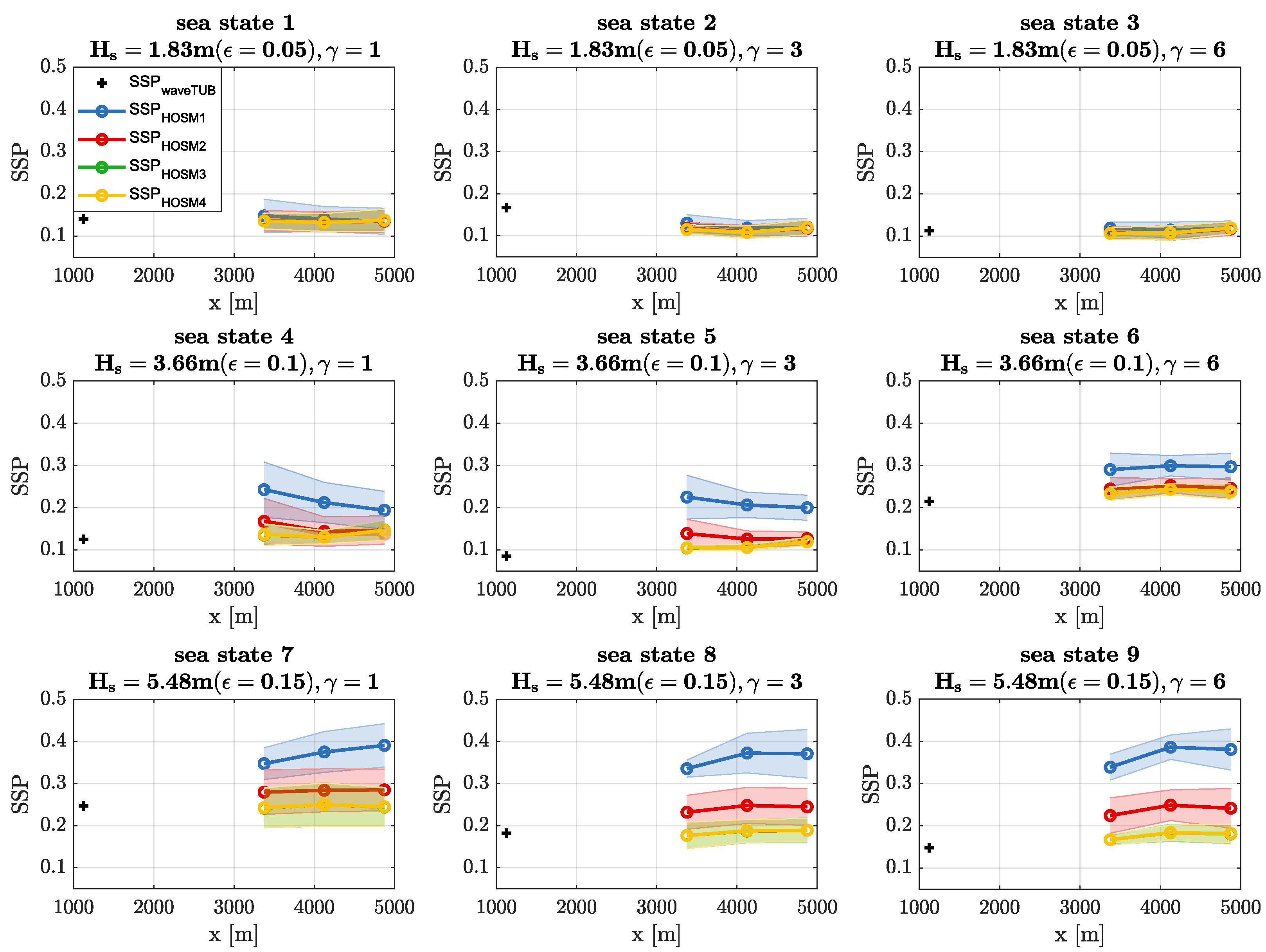
Figure 6 shows the accuracy of the HOS simulations compared to the measurements for irregular sea states (cf. Table 2). It presents the $\mathrm{SSP}$ of the waveTUB input snapshot (black plus), as well as simulations with HOSM1 (blue curves), HOSM2 (red curves), HOSM3 (green curves), and HOSM4 (yellow curves). The points on the curves indicate the positions of the three wave gauges (cf. Figure 5). The $\mathrm{SSP}$ shown is the average of the eight consecutive snapshots per sea state, and the transparent area around each curve (of the same color) represents the variance corresponding to the eight simulations. The $\mathrm{SSP}$ for the waveTUB input snapshot was calculated for the whole time trace at Wave Gauge 1. Again, the horizontal diagrams depict sea states with constant wave steepness and increasing enhancement factor from left to right. For sea states vertically aligned, the enhancement factor is kept constant and the wave steepness increases from top to bottom.

It can be seen that the basic findings from the numerical investigations (Figure 2) are mainly verified by the experimental results—the accuracy of HOSM1 and HOSM2 decreases with increasing wave steepness, and the accuracy of HOSM3 is almost identical to that of HOSM4.

However, for the wave steepness $ϵ=0.05$, the results of the numerical investigations differ from the experimental ones. In contrast to the numerical results, in which significant differences between the different orders can already be seen at this steepness (cf. Figure 2), all orders show approximately the same accuracy compared to the experimental results (cf. Figure 6). This is most likely due to the fact that the input snapshot already has a certain inaccuracy, which is why simulating with a low order makes comparatively less difference. Overall, experiments of this kind are important, but individual effects of different sea state parameters become more apparent in the controlled environment of numerical simulations.

6. Conclusions

In this paper, the influence of characteristic sea state parameters of the JONSWAP spectrum on the accuracy of simulations with varying complexity was investigated. For this purpose, both purely numerical and experimental data were used to systematically assess the accuracy of HOS simulations of different orders up to the fourth one. In the case of numerical data, the fourth-order solution HOSM4 served as the reference to evaluate the accuracy of the lower-order solutions. In the semi-experimental configuration, probe measurements from wave tank experiments were used as the reference solution. In both cases, the comparison was made by means of the $\mathrm{SSP}$ calculated between the reference solution and the HOS solutions at different orders.

The numerical investigation showed that for small wave steepnesses ($ϵ\le 0.0375$), the first- and second-order solutions (HOSM1 and HOSM2, respectively) had a sufficient accuracy. When the steepness increased, however, the nonlinear effects became dominant, resulting in a significantly decreased accuracy for both orders. On the other hand, the third-order solution HOSM3 remained almost similar to the reference over the entire parameter space, with an $\mathrm{SSP}$ value far below the threshold $\mathrm{SSP}\le 0.1$ even in the most unfavorable configuration of $ϵ=0.125$ and $\gamma =1$, and after 25 peak periods of propagation. Longer simulation times validated the trends obtained for 25 peak periods of propagation by showing an almost linear increase of $\mathrm{SSP}$. This confirms that most of the relevant nonlinear effects pertain to third-order terms. Although the peak enhancement factor appeared to influence the simulations’ accuracy (i.e., higher $\mathrm{SSP}$ for lower $\gamma$), the directional spreading factor had almost no effect on the results.

The experimental investigation generally confirmed the numerical observations: the higher the wave steepness, the higher the $\mathrm{SSP}$ and the larger the difference between each HOS solution, except for HOSM3 and HOSM4, which led to almost identical results.

Overall, it was shown that for certain irregular sea state parameters, i.e., less steep wave systems, low-order solutions provide sufficient accuracy. Due to the lower numerical effort associated with less complex solutions, time can be saved by choosing the order of complexity depending on the sea state parameters.

Future work on this topic should focus on the water depth and possible influences on the accuracy of the different orders. In addition, the influence of the peak enhancement factor, in particular the underlying physics for the observed influence, should also be addressed in future studies.