Abstract
Using variational mode decomposition, we analyze the signal from velocities at the center of the channel of a microfluidics drop-maker. We simulate the formation of water in oil droplets in a microfluidic device. To compare signals from different drop-makers, we choose the length of the water inlet in one drop-maker to be slightly shorter than the other. This small difference in length leads to the formation of satellite droplets and uncertainty in droplet uniformity in one of the drop-makers. By decomposing the velocity signal into only five intrinsic modes, we can fully separate the oscillatory and noisy parts of the velocity from an underlying average flow at the center of the channel. We show that the fifth intrinsic mode is solely sufficient to identify the uniform droplet formation while the other modes encompass the oscillations and noise. Mono-disperse droplets are formed consistently and as long as the fifth mode is a plateau with a local standard deviation of less than 0.02 for a normalized signal at the channel inlet. Spikes in the fifth mode appear, coinciding with fluctuations in the sizes of droplets. Interestingly, the spikes in the fifth mode indicate non-uniform droplet formation even for the velocities measured upstream in the water inlet in a region far before where droplets form. These results are not sensitive to the spatial resolution of the signal, as we decompose a velocity signal averaged over an area as wide as 40% of the channel width.
1. Introduction
Droplet microfluidics is a powerful technique enabling the precise control of the size of the droplets, loading of cargo, sorting, and merging droplets at small volumes of the order of picolitres. These capabilities have led to the extensive use of droplet microfluidics in a wide range of applications in industries such as in pharmaceutical, material production, and in research and development [1,2,3]. Moreover, droplet microfluidics is a promising tool in signal processing [4,5]. The sizes of the droplets are determined by the interfacial tension between the two fluids, the geometry of the microfluidics chip, and the flow rates of each fluid phase [6,7]. Microfluidics chips operated in their optimum regime prove to be stable and reliable for the production of monodisperse droplets [8,9,10,11,12]. On-chip processes can be optimized to minimize errors in performance since a microfluidic chip interacts with a few external control units, pumps, and valves [13]. However, small errors, such as satellite droplets, missed mergers, or unexpected merging of droplets may still occur due to instabilities in external units or in local flow [14,15]. In general, these errors are monitored visually and anomalies can be sorted out with different methods, either by deflecting some fluids to a separate channel using external electric or acoustic forces or by passing the droplets through filters to sort by size [5,16,17]. Since most microfluidics chips run at high speeds, 100 s of L/h [15], it is crucial to detect and correct errors at comparable speeds. Flow fluctuations in a microfluidic channel driven at a high flow rate can grow quickly and disrupt the flow downstream due to the nonlinear nature of fluid flows. Although not all fluctuations are significant, it is not possible to identify them theoretically or in real time once a microfluidic device is running. Nevertheless, flow velocities and pressure fluctuations in a device are accessible in real time [18,19].
In principle, standard methods of signal processing can be implemented to quantify or predict anomalies in microfluidics, although they are not commonly used. Fourier transform and wavelet analysis perform well in simplifying complex and noisy time series. However, this powerful signal analysis method is less efficient in nonlinear and non-stationary systems such as fluid flows and can be computationally intense. Moreover, dynamic mode decomposition is developed based on continuous snapshots of flow and is shown to closely describe the motion of the flow even in the turbulence regime [20]. In recent decades, the empirical mode decomposition (EMD) method has been developed to better analyze signals from nonlinear and non-stationary data sets [21,22,23]. EMD is data driven, a posteriori, and adaptive, which aims to separate events by utilizing the notion of instantaneous frequency, in contrast with fundamental frequencies as in Fourier analysis. EMD has been used in a variety of applications, including identification of dominant frequencies in atmospheric data [24], separating unsteady spatiotemporal scales in the mixing layer in wind tunnel data [25], analyzing instantaneous turbulent velocity field in unsteady flows [26], and extracting health-related hemodynamics features [27]. One of the successful uses of EMD is to identify modes or frequencies with physical significance in a noisy signal, as in characterizing the properties of turbulence from stationary and non-stationary grid-generated flows [28]. For example, in a systematic study, a periodic perturbation was introduced to the flow, and EMD was used to separate the high-frequency part of the signal from the low-frequency parts, and the artificial perturbation was retrieved. Variational mode decomposition (VMD) has been developed based on EMD with a lower sensitivity to noise [29]. This method stepped away from recursive decomposition and extracts modes concurrently. It finds central frequencies and oscillatory modes within various basebands [29], and is even proven to extract central data from geophysical data where isolated spikes appear often [30,31]. The applications of VMD in different areas of fluid mechanics and hydrodynamics has been extremely promising in isolating physical signals and providing predictive metrics for improved performances [32,33,34,35].
In this paper, we use a novel method of signal decomposition, variational mode decomposition, to determine the formation of uniform droplets in a microfluidic drop-maker. We simulate the formation of water in oil droplets in a microfluidic device with two independent drop-makers. To compare the signal from different geometries, we choose the sizes of the water inlets of the drop-makers to be slightly different. We map the velocities calculated in the simulation onto a uniform grid to mimic the velocity field commonly measured in experiments using particle image velocimetry. Using variational mode decomposition, we decompose the velocities measured at the center of the channel to its intrinsic mode functions (IMF). For the velocity signal in our simulations, only five modes are sufficient to fully separate noise and high oscillations from the underlying average velocity. The first mode in the decomposition, IMF 1, usually has the highest oscillations and noises among all modes. The second to fourth modes have considerable oscillations with magnitudes similar to each other and similar to the first mode or at least within the same order of magnitude. However, the fifth mode, IMF 5, appears to only show the underlying average velocities at the center of the channel with values much larger than the other IMFs. We find that uniform droplets form when IMF 5 is a plateau with small variations around its local average. Interestingly, this signature plateau coincides with uniform droplet formation even when we use the velocities inside the water inlet and long before the fluid is broken into droplets. We show that variational mode decomposition is able to quantify anomalies in the signal that trigger fluctuations in flow and droplet sizes downstream.
2. Materials and Methods
2.1. Droplet Simulation
To study the flow fluctuations during droplet formation in a microfluidic T-junction with high spatial resolution, we use COMSOL multiphysics (3.2.10), a laminar two phase flow module, and the level set method [36]. The geometry of the microfluidic device consists of two T-junction dropmakers located on opposite sides of a long channel. Droplets are generated on two sides of this channel and meet in the middle of the device where they can either merge or bypass each other and exit through a single outlet as shown in Figure 1 (Supplementary Materials). The widths of the inlets channels are 50 m. Droplets are formed when the inner fluid, water, in the middle inlet is sheared with the outer fluid, an oil which has an interfacial tension of = 3 mN/m with water [36], which flows in the two adjacent inlets as shown in Figure 1 (Supplementary Materials). Here, we choose to generate water in oil emulsion droplets. The density of the inner fluid, , is 1 kg/L and the outer fluid is 1.6 kg/L and their respective viscosities are = 1 mPas and = 1.2 mPas. To keep the simulations stable and resolve the interfaces, COMSOL used an adaptive mesh with nonuniform grid sizes. The lengths of the channels on either side are 425 m, measured from the beginning of the inlet. These lengths are optimized so the two-phase simulation is stable and the interfaces are resolved while the microfluidic device resembles physical experiments [1]. The inner fluid is flowed at 2 cm/s and the outer fluid at u = 2 cm/s. At these flow rates, a steady stream of droplets is expected to form in the dripping regime [7]. The imposed pressure at outlet is = 0 Pa. The capillary number is , ratio of capillary to viscous force (). The corresponding Weber number, the ratio of drag to cohesion force, is , where r is the radius of the channel. The Capillary and Weber numbers are within the dripping regime where the balance between the capillary forces at the interface of two fluids and the viscous force from the outer fluid determines the formation of a droplet [7]. Once a droplet is formed, it flows through the channel leading to the junction with the opposite dropmaker as shown in Figure 1 (Supplementary Materials). The left inlet channel is shortened to mimic a fabrication error while the right channel has an optimized geometry for the flow rates chosen. The left channel begins to form droplets a few milliseconds before the right channel as well as form satellite and non-uniform droplets sporadically. The numerical simulation in COMSOL uses an adaptive mesh to optimize the computational time. Consequently, the data are on a non-uniform grid with finer mesh sizes close to the interfaces. Using the natural neighbor algorithm, we interpolate this data on a uniform grid. The mesh size is 200 nm and the total area of the mesh is 850 × 215 m.
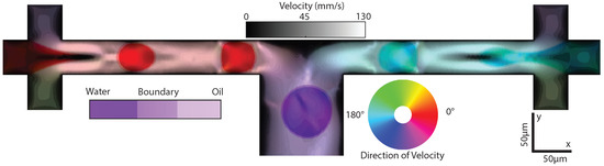
Figure 1.
Visualization of two-phase fluid and flow velocities in a microchannel where droplets generated from right and left drop-makers meet at the center of the channel. Color Hue represents direction of the velocity, Saturation represents the volume fraction of water, and brightness Value represents the magnitude of the velocity.
2.2. Signal Decomposition
Variational mode decomposition extracts oscillatory modes of the signal and provides insight into how the flow evolves as a function of time at various positions. VMD is a modern algorithm based on some of the concepts of empirical mode decomposition which were first developed with nonlinear and non-stationary processes in mind to decompose a time-domain signal into intrinsic mode functions [21,37]. These oscillatory modes, IMF, follow two primary criteria: (i) the number of extrema and number of zero crossings must either be equal or only differ by one; this criteria is equivalent to the narrow band requirement for a stationary Gaussian process. (ii) The mean value of the envelope defined by the local maxima and minima must be zero [38]. The second criterion creates a local time-dependent requirement which assists with decomposing nonlinear signals and allows IMFs to have both modulated amplitude and frequency with a finite bandwidth. However, boundaries and spikes in the original signal can lead to artifacts in the IMFs to satisfy the criteria mentioned above. To resolve such issues, various methods have been developed among which variational mode decomposition (VMD) has been successfully used to describe dynamics in fluid systems [31]. VMD stepped away from recursive decomposition and extracts modes concurrently. It searches through frequencies of the original signal to find central frequencies and oscillatory modes within various basebands [29]. VMD adaptively selects the IMFs concurrently, which results in modes covering finite bandwidth within the original signal. Being weighted towards central frequencies, IMFs contain physically relevant information of various processes that influence the original signal, see Appendix A. In this paper, we use the MATLAB (R2020a) built-in variational mode decomposition function to decompose the velocity, u(t), at a given space into its oscillatory modes. The number of IMFs needed to decompose the signal into physically relevant modes is not known a priori. We vary the number of IMFs between 4 and 6 to decompose the signal. We find that five IMFs are sufficient throughout our data to decompose the signal without any redundancy or loss of modes that appear significant in predicting the droplet dynamics. Increasing the number of IMFs affects the decomposition noise and oscillatory components which are of less interest in this system in the laminar regime.
The goal is to analyze the flow dynamics in a time-domain signal to find a signal that will allow us to determine if uniform droplets are being created at certain instances by viewing a single region within the inlet. This is in contrast with other methods of signal analysis in fluids such as dynamic mode decomposition which require a much larger data set in the entire field.
3. Results
We develop a consolidated visualization method that integrates multiple physical quantities, velocity, and fluid phase, into a simple graphic to better identify different dynamics. To visualize the direction and magnitude of fluid velocities along with the volume fraction of each fluid phase, corresponding colors, intensities, and saturation are assigned to form a single HSV image (Hue, Saturation, Value) as shown in Figure 1 (Supplementary Materials). Hue is determined by the angular velocity at each position and is mapped to a 360-degree color wheel with red and cyan corresponding to 0 and 180 degrees, respectfully. Saturation represents the volume fraction of oil and water. Saturation is 1.0, where the volume fraction of water is larger than 55% and 0.25 where the volume fraction is smaller than 45%. Saturation matches the volume fraction of water everywhere else as shown in the Saturation color bar in Figure 1 (Supplementary Materials). Moreover, the magnitude of the velocities is represented by Value, which describes how light or dark a Hue is with larger velocities appearing brighter. Since there is an uneven distribution of velocities, with many small velocities and a few large velocities, there is poor contrast within the slow velocity regions. To enhance the contrast in these regions, we use a global transformation that bins and maps velocities across all spatial and temporal points into Values. However, the distinction between the few high velocities is no longer visible. This transformation and mapping, known as histogram equalization, aims to create a uniform probability density function that enhances contrast for tightly grouped velocities. Although it is unlikely to create a completely uniform histogram, histogram equalization generally results in a wider range of the intensity scale to be used and, consequently, the contrast is enhanced [39]. This process is only used for the visualization of the data and the velocities after histogram equalization are not used in data analysis.
Droplets of water in oil are formed on either side of the long channel and carried by the outer fluid (oil) as shown in Figure 1 (Supplementary Materials). Droplets formed in the left channel appear red as they travel from left to right. These droplets meet droplets from the opposing channel at the T-junction. Droplets either merge or deflect towards the outlet vacating the device while appearing purple due to their now downwards velocity. Interestingly, we observe a considerable number of satellite droplets in the left channel where we intentionally selected non-ideal inlet geometry. Consequently, the sizes of the droplets from the left channel are less uniform and the dynamics at the point of merging become unpredictable with many missed mergers as observed in Figure 1 (Supplementary Materials).
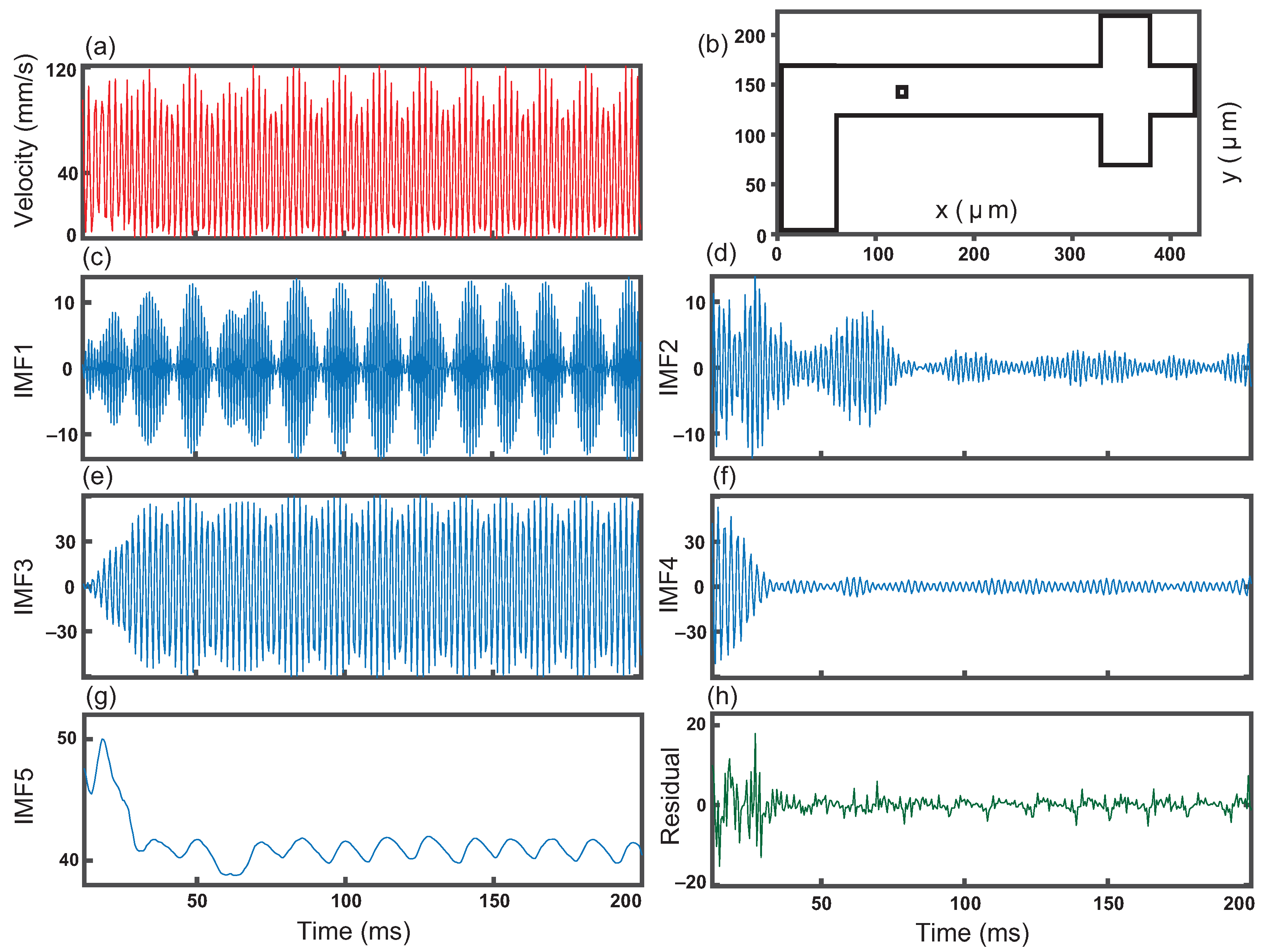
We use variational mode decomposition to analyze temporal flow fluctuations downstream and identify any significant modes. We choose a region of 4 × 4 m in the right channel, 290 m downstream, to investigate where there is less variation in flow velocity away from the inlets prior to the outlet, as shown in Figure 2b. We calculate the average flow velocity in this region since our velocity field has a resolution of 200 nm, which is not achievable in most experiments.

Figure 2.
Velocity and decomposition at one position as a function of time. (a) Magnitude of velocity from 12 to 200 ms (b) for a 4 × 4 m bin in the center of the channel; (c) First intrinsic mode function (IMF 1) of the decomposed velocity signal showing the fastest oscillations in the original signal; (d) IMF 2, the second largest oscillations heavily affected by the initiation of flow; (e) IMF 3 showing the bulk of the original velocity signal; (f) IMF 4 slower oscillations with a transition at around 20 ms corresponding to the initiation of flow; (g) IMF 5 is the slowest oscillation of the flow with an average close to velocity of the outer fluid at 40 mm/s, and a spike early in the signal at time briefly after the initiation; (h) Residual of the signal.
Interestingly, droplets pass this region with very little variation in size and shape. We utilize variational mode decomposition to separate fluctuations from the steady flow of droplets and drop formation. Various regions require a different number of modes to produce unique IMFs without frequency and amplitude overlap. We choose five intrinsic mode functions for this position for all IMFs to remain significant and residual to have minimal oscillation. From our visualization of the right channel in Figure 1 (Supplementary Materials), no major fluctuations are expected since we see consistent production of uniform droplets. However, IMF 2 and 4 have a large amplitude present at the start of the signal which wanes later in the signal. The maximum amplitude of IMF 2 (IMF 4) from 0 < t < 80 ms ( 0 < t < 25 ms) is 4.73 (8.83) times greater than the maximum amplitude in the rest of the IMF. The simulation begins with the device filled with oil. Therefore, there are fluctuations in the velocities due to water being introduced to the device. We consider this an initiation stage for the flow. The effect of the initiation of flow is present in IMFs 2 and 4. The amplitude in IMF 3 appears to be modulated periodically, which we attribute to the steady flow of droplets. IMF 5 summarizes both the effect of initiation of flow as well as the periodicity from the flow of droplets. Moreover, the sharp drop in the amplitude in IMF 5 matches the time when IMF 3 transitions to a periodic signal. Additionally, this time is close to where initiation effects in IMF 4 start to wane. The decomposition clearly separates the events affected by the initiation of flow, which appear in IMF 2 and IMF 4, and the steady flow and drop formation that are evident in IMFs 1, 3, and 5. Interestingly, IMF 5 has some of the initiation effects which are distinct peaks matching the IMF 2 and IMF 4 as well as the fluctuation within relatively consistent signals in IMF 1 and IMF 3 at around 60 ms. The residual does not have any significant physical meaning (Figure 2h), except that the signal can be recovered exactly by adding the residual and all other IMFs.
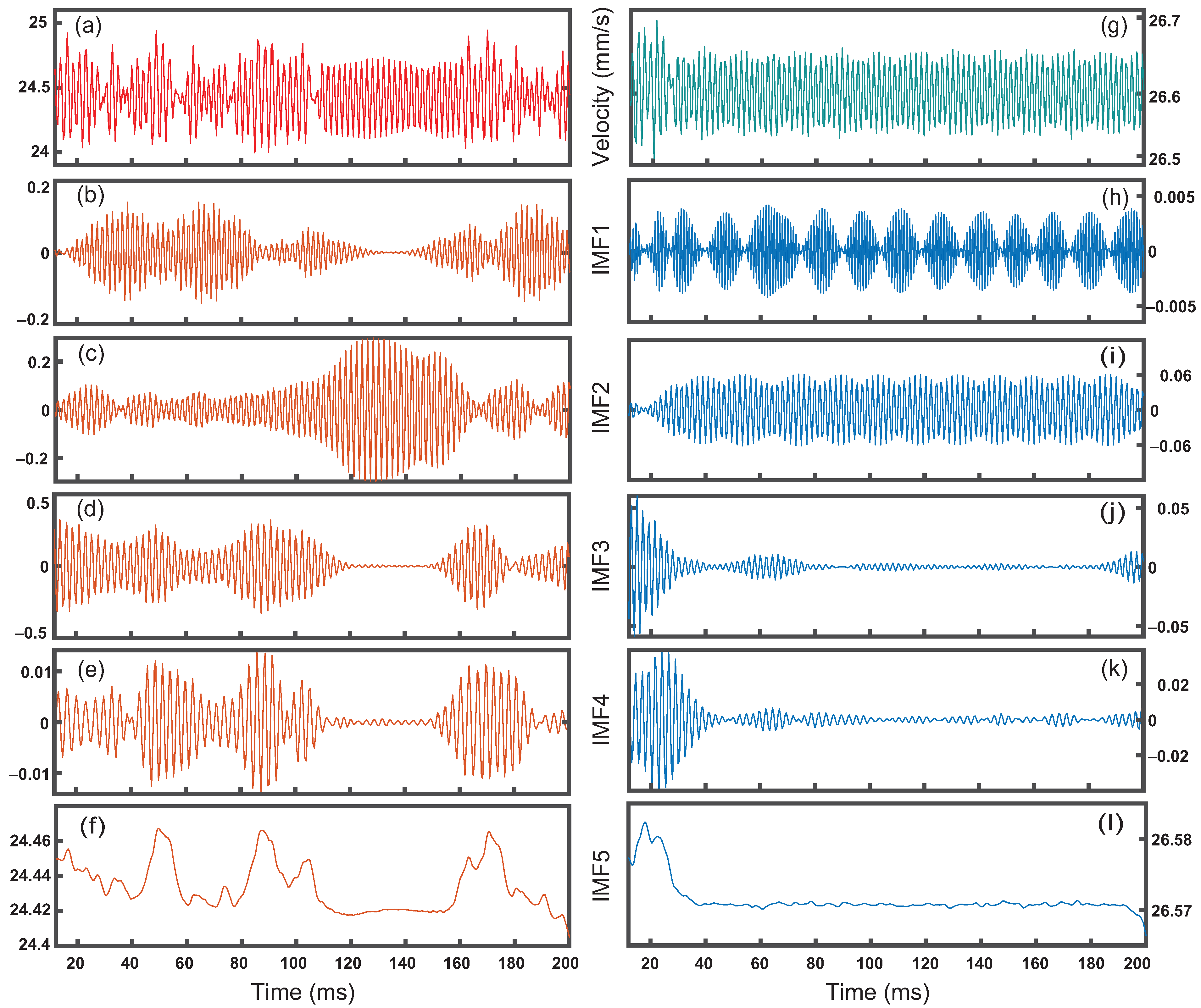
Using variational mode decomposition, we analyze temporal flow fluctuations at both water inlets and identify any significant modes that indicate changes in droplet formation. We calculate the velocity signal and IMFs of 4 × 4 m regions prior to the oil inlets and pinch off points, 20 m into the water inlets, for the left and right drop-makers shown in Figure 3. Interestingly, we observe that the right channel signal and IMFs appear similar to the results found downstream, comparing Figure 3h–k to Figure 2c–f. The periodicity in IMF 2 coincides with the steady flow of droplets while IMF 3 and 4 show the effects of initiation. Here, IMF 1 is an order of magnitude smaller than the other IMFs. Additionally, IMF 5 contains a peak close to the initiation of the flow and the amplitude falls off close to the average flow velocity after the initiation. We observe that there is almost no periodicity in IMF 5 which is different from data downstream where droplets continuously pass through. The decomposition of the signal for the left channel at the water inlet leads to IMFs with highly variable amplitudes. The amplitudes of IMFs 1 to 3 are comparable to each other and are larger than that of IMF 4, as can be seen in Figure 3b–e. We observe multiple large peaks in IMF 5 which are of the same order of magnitude as the effect due to the initiation of flow. By contrast, there is a plateau in IMF 5 during the time interval, 115 < t < 155 ms. Interestingly, this plateau in IMF 5 coincides with the formation of uniform droplets from the left channel. Moreover, during this time interval, the amplitude of IMF 3, which has the largest range among all IMFs, is at its minimum. IMF 4 is also at its minimum during this time interval. We observe that IMF 2 during this time interval has a behavior similar to what is seen in uniform droplet formation in the right channel. Additionally, IMF 2 contains most of the original signal during this time interval. Satellite and non-uniform droplets are formed in the left channel at all other times. The effect of initiation is apparent in IMF 3 and 4 in the right channel, Figure 3j,k, while, in the left channel, this effect is not the most significant change in amplitude in any of the IMFs, Figure 3d,e, and becomes suppressed. It should be noted that the signal obtained from the left water inlet ranges between 1 mm/s while the signal from the right channel ranges 0.2 mm/s. Additionally, IMF 1 for the left channel (Figure 3b) has amplitudes an order of magnitude larger than that seen in IMF 1 of the right channel (Figure 3h). IMF 1 contains the highest oscillating component of the signal which is typically attributed to noise in the system.
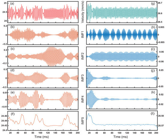
Figure 3.
Velocity and decomposition in the water inlet as a function of time. Left: the velocity signal (a) and decomposition into intrinsic mode functions (b–f) for the left channel of Figure 1 (Supplementary Materials) demonstrates various large fluctuations. Right: velocity signal (g) and decomposition (h–l) for the right channel with a single large fluctuation.
Our analysis of the decomposed signal demonstrates and predicts if uniform and non-uniform droplets will be formed; surprisingly, our prediction is based on the signal in the region before where droplets are pinched off. Naturally, it is difficult to predict the formation of uniform droplets from this region. We identify characteristics in the decomposed signal that indicate time intervals when uniform droplets are formed. It appears that the peaks in IMFs 3 and 4 mostly coincide with fluctuations that destabilize the formation of uniform droplets. Uniform droplets are formed whenever there is a plateau in IMF 5. To better define the plateau, the average and standard deviation of the IMF 5 are calculated on a moving window of at least 7 ms, corresponding to the time needed to form two droplets. The fluctuations in the IMF 5 can be ignored as long as this local standard deviation is smaller than 0.02. To predict if a uniform droplet is formed, we calculate the standard deviation of IMF 5 over 7 ms before this time-step, assuming we have no information about future velocities.
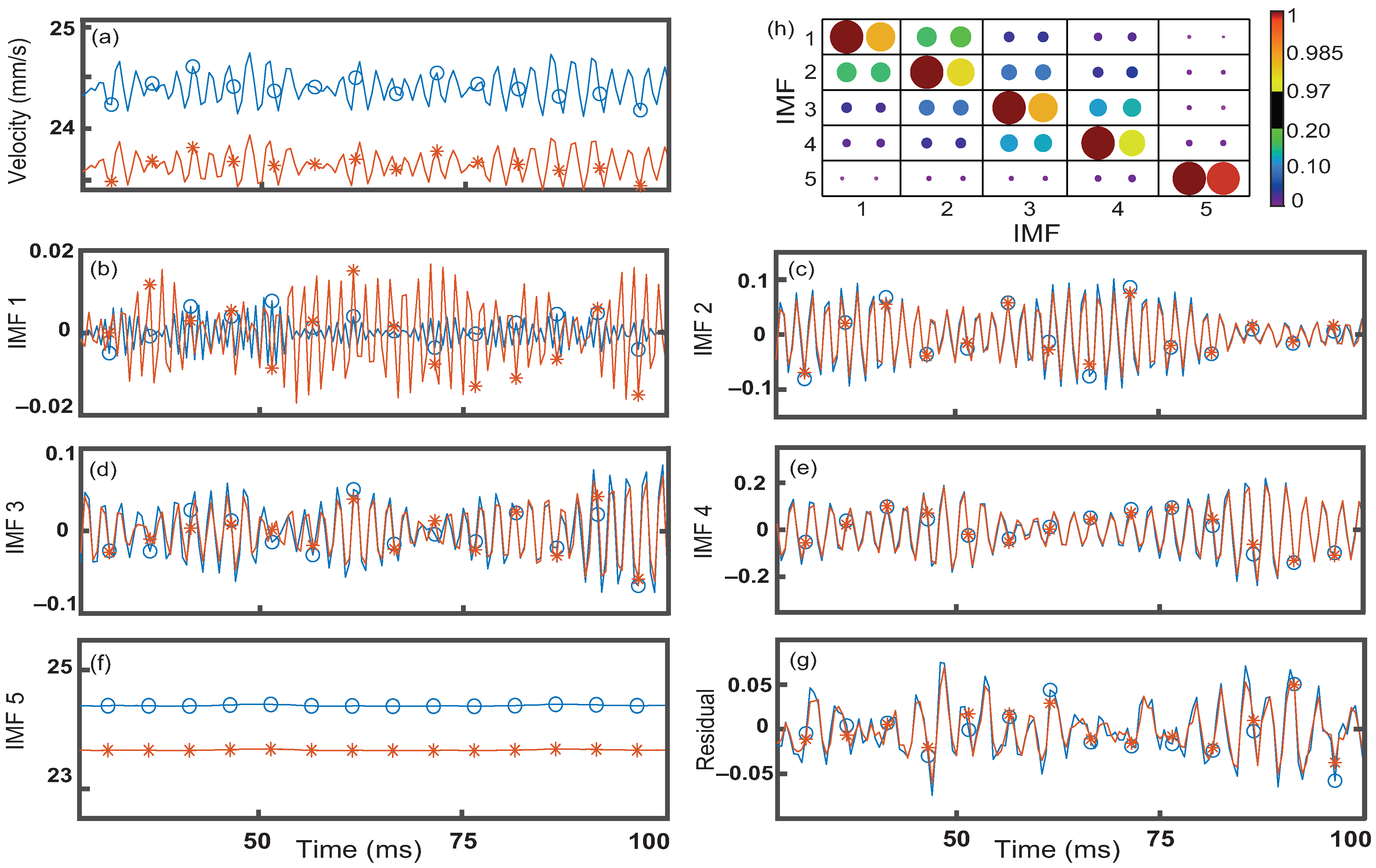
To investigate the applicability of the signal decomposition in lower resolution data, we study the relationship between various spatial resolutions of the signal and decomposition. Additionally, this helps with evaluating the relevance of this method for experimental data considering simulations that generally have higher spatial resolutions than in experiments. We analyze two velocity signals taken from the same position, centered between the oil inlets, at different resolutions ranging from 4 × 4 to 20 × 20 m. To quantify the similarities in the IMFs, we calculate the maximum normalized cross-correlation of the above signals with the signal obtained from a 1 × 1 m region (5 × 5 pixels):
where i and j represent the IMF number, and n and m are the elements in each IMF. The superscript (1) and (2) represent the different resolutions of the data. In our calculations, we choose (1) to be at the 1 × 1 m resolution and vary (2) between 4 × 4 m and 20 × 20 m. Here, is an array with values between −1 and 1. We expect, for at a coincident time, to be highly correlated. However, on rare occasions there is a time lag between the signals because we are averaging over a larger window that encompasses fluid elements in nearby locations. Hence, we report the maximum of this array for every combination of IMFs.
Comparing the velocities averaged over a 4 × 4 and 20 × 20 m region centered between the two oil inlets, we find that the higher resolution has larger average velocities. This is natural since the lower resolution signal is averaging velocities closer to the wall, which are slower velocities than the center, as seen in Figure 4a. The different IMFs from the two resolutions are barely different in amplitude and frequency from one another as seen in Figure 4b–g. Small differences are observed in IMF 1, which is an order of magnitude smaller than the other modes, Figure 4b. We attribute these differences at this position to the 20 × 20 m window extending into the water channel which has additional inlet noise. Our calculation of the maximum demonstrates that the coinciding IMFs are highly correlated regardless of spatial resolution, Figure 4h. Additionally, non-coinciding IMFs have very little correlation as demonstrated by the extremely small and negligible sizes of the correlation bubbles in Figure 4h. The lowest maximum of the coinciding IMFs is 0.97 seen for IMF 4 of the 20 × 20 m region. It is apparent that the results of the decomposition are weakly dependent on spatial resolution up to 20 × 20 m when using a 1 × 1 m region. Our results imply that this method should work on lower resolution experimental data. Additionally, IMFs 2 to 4 and the residual match closely between the two different resolutions.
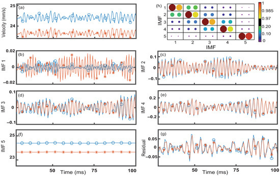
Figure 4.
Velocity signal (a) taken at a single position averaged for two different resolutions, 4 × 4 m (blue circles) and 20 × 20 m (orange asterisk); (b–g) the respective Intrinsic mode functions; (h) normalized maximum cross correlation between the IMFs of the 4 × 4 m (left) and 20 × 20 m (right) with a 1 × 1 m region. Color bar and relative size represent the strength of the correlations.
To verify the robustness of this method, we calculate the maximum normalized cross-correlation, , across the center of the channel averaged for different positions. To avoid overlaps of the larger window, we choose these positions to be 65 m apart. We calculate the for the signal obtained from a 1 × 1 m window correlated with the 4 × 4, and the 20 × 20 m windows. Interestingly, IMF 5 remains highly correlated regardless of window size and position in the channel as shown in Table 1. Coinciding IMFs are heavily correlated for the 4 × 4 m window size with very little correlation amongst non-coinciding IMFs, as can be seen by comparing the diagonal elements of Table 1 with the off-diagonal elements. These results clearly show that the 4 × 4 m window is small enough and the decomposed signal matches the 1 × 1 m window closely (max). However, the for i = j for IMFs 2, 3, and 4 are less correlated for the larger window size, 20 × 20 m. Here, the off-diagonal elements () increase as seen in Table 2.

Table 1.
Maximum normalized cross correlation averaged over 12 positions with areas of 4 × 4 m region. The IMF 1 to 5 on the columns are from the 1 × 1 m and the rows are from the 4 × 4 m.
Table 2.
Maximum normalized cross correlation averaged over 12 positions with areas of 20 × 20 m. The IMF 1 to 5 on the columns are from the 1 × 1 m and the rows are from the 20 × 20 m region.
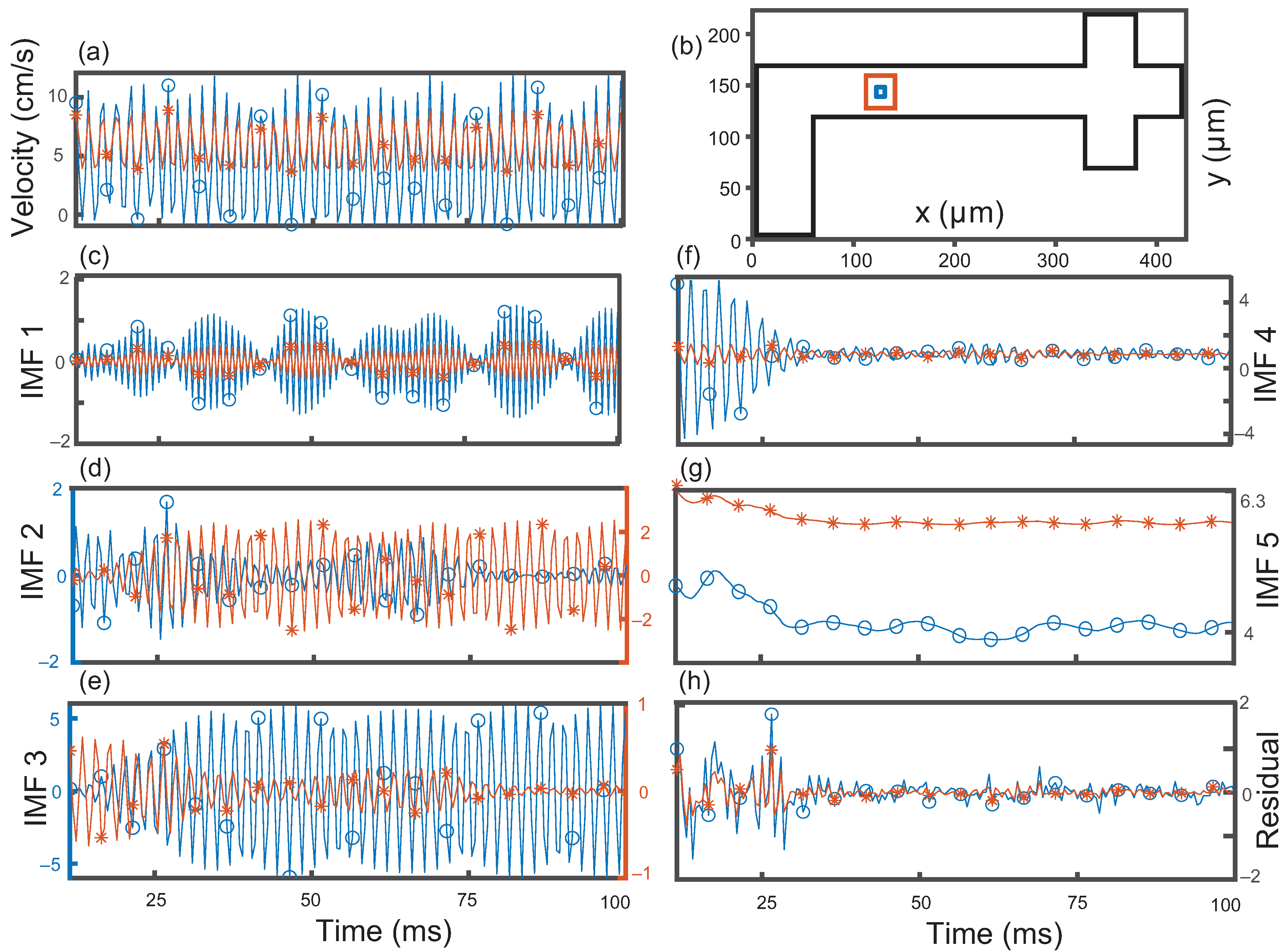
Upon further investigation, IMF numbers swap occasionally when decomposing signals from different window sizes or neighboring positions. An example of this swapping is demonstrated for two window sizes (4 × 4 and 20 × 20 m) at the center of the channel in Figure 5. Here, swapping IMFs 2 and 3 of the larger window would result in a greater . Interestingly, this swapping seems to be contained to IMFs 2, 3, and 4. These three IMFs are small in magnitude and similar in frequency where small changes in the average signal can swap their assigned IMF number. Additionally, the swapping is predominately amongst neighboring modes, IMFs 2 and 3 and IMFs 3 and 4 swapping. The prevalence of swapping increases with window size as additional velocities further from the center of the channel are being averaged into the signal prior to decomposition. However, IMF 1 remains highly correlated regardless of window size up to 20 × 20 m. The most consistent mode is IMF 5 as it was heavily correlated (Max) even when using a 20 × 20 m window size at various positions. We observe that IMF 5 is a good indicator for changes in droplet formation and remains strongly correlated regardless of the spatial resolution tested.
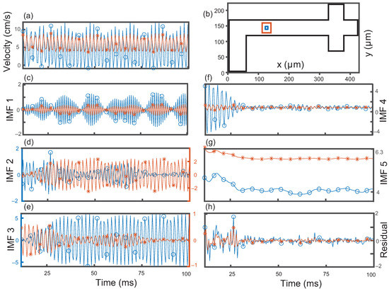
Figure 5.
Velocity signal and decomposition at one position as a function of time. (a) magnitude of velocity from 12 to 200 ms (b) for a 4 × 4 m (blue circles) and 20 × 20 m (orange asterisk) window size at the center of the channel; (c) first intrinsic mode function (IMF 1); (d) IMF 2 where the larger window decomposition swaps with IMF 3; (e) IMF 3 where the larger window swaps with IMF 2; (f) IMF 4; (g) IMF 5, (h) Residual.
4. Discussion
We simulate the formation of water in oil droplets and extract a high resolution velocity field from the simulation. In this microfluidic drop-maker, we incorporate two independent drop-makers with slightly different inlet geometries—in one of which the inlet is shorter than the other. The short inlet leads to the formation of satellite droplets at the same flow conditions as the other inlet. Using variational mode decomposition, we decompose the velocity signal at the center of the channel into its intrinsic modes. We show that, by only decomposing the signal into five intrinsic modes, we can fully separate the oscillatory and noisy parts of the velocity from an underlying average flow at the center of the channel. Interestingly, IMF 5 carries most of the physical information. IMF 5 has distinct spikes when the flow is initiated and it transitions into a plateau as long as the droplets are uniform. The IMF 5, of variational mode decomposition, has a smooth shape when uniform droplets are formed even if we analyze the velocities in the water inlet and before the region where droplets form. Additionally, this method is not sensitive to the spatial resolution of the signal, as we decompose a velocity signal averaged over a considerably large area. We show that magnitude of IMF 5 remains to be highly correlated with the high resolution velocities further confirming the robustness of prediction of flow fluctuations by IMF 5. By choosing the appropriate number of modes, we efficiently separate the physical part of the signal from oscillatory and noisy parts. Our analysis provides a metric to predict uniform and satellite droplet formations.
The variational mode decomposition is a promising method of signal decomposition suitable for fluid flows with random or periodic fluctuations. Additionally, VMD is integrated into scientific software such as MATLAB, making it readily accessible to a broad range of users. Moreover, VMD can be applied to spatially sparse data without losing critical information about the underlying signal, as we demonstrate in this paper. While some of the conventional methods of signal analysis, such as Fourier transform and Dynamic mode decomposition, have been used in different areas of fluid mechanics, mainly in turbulence and channel flows, the use of signal analysis in microfluidics has received less attention. Nevertheless, the integration of microfluidics circuits in commercial platforms for sorting and processing small volumes of fluids is rapidly growing. Hence, the application of signal analysis in microfluidics for optimization, troubleshooting, and quality assessments is on the rise. Here, we demonstrate the successful application of VMD in predicting droplet sizes and provide a platform for future use of VMD in microfluidics signal analysis. Future exploration of the application of this method and extension into experimental and real time analysis can improve the performance of microfluidics chips with single point velocity monitoring.
Supplementary Materials
The following supporting information can be downloaded at: https://www.mdpi.com/article/10.3390/fluids7050174/s1, Movie S1: Simulation Visualization.
Author Contributions
Conceptualization, M.I., L.N., and S.P.; methodology, M.I. and S.P.; validation, M.I., L.N., and S.P.; formal analysis, M.I. and S.P.; investigation, M.I. and S.P.; resources, S.P.; data curation, M.I. and S.P.; writing—original draft preparation, M.I. and S.P.; writing—review and editing, M.I. and S.P.; visualization, M.I.; supervision, S.P.; project administration, S.P.; funding acquisition, S.P. All authors have read and agreed to the published version of the manuscript.
Funding
This work was supported by the the Donors of the American Chemical Society Petroleum Research Fund, Grant No. ACS-PRF 62566-DNI9, and the R.I.T. College of Science: Dean’s Research Initiation Grant. L.N. acknowledges support from the Emerson Summer Undergraduate Fellowship from the R.I.T. College of Science.
Data Availability Statement
The data for this study are available from the corresponding author upon reasonable request.
Acknowledgments
Acknowledgment is made to the Donors of the American Chemical Society Petroleum Research Fund for support of this research.
Conflicts of Interest
The authors declare no conflict of interest.
Abbreviations
The following abbreviations are used in this manuscript:
| EMD | Emprirical Mode Decomposition |
| VMD | Variational Mode Decomposition |
| IMF | Intrinsic Mode Functions |
Appendix A. Variational Mode Decomposition
Variational mode decomposition separates a signal into components that can be expressed mathematically as amplitude-modulated-frequency-modulated signals [29]. This is in contrast with Fourier transform which describes a signal as a sum of non-varying sinusoidal functions. A mode, , in VMD is described as
where A is the time-dependent amplitude and is the phase. Decomposing a signal into functions that can vary over time allows VMD to become locally adaptive and have the ability to act as a narrow band filter. The robust nature of such a decomposition method effectively allows VMD to decompose signals from nonlinear and non-stationary systems [29]. A real function can be represented as an analytic signal that is comprised of the original function and its Hilbert transform as:
Here, is the Hilbert transform of the signal, represents the analytical representation of the signal, and is the instantaneous amplitude and envelope of the signal. Instantaneous frequency is found by the rate of change of the . The mode can be expressed as analytic signals. This allows us to represent the mode in the form of a complex exponential with no negative frequencies:
In summary, variational mode decomposition utilizes frequency mixing and Hilbert transforms to extract narrow band functions from a signal [29]. This minimization problem is framed by attempting to simultaneously finding a unique number of functions, or modes, around different central frequencies that sum to the original signal. These central frequencies, , are initialized randomly or selected and are then mixed with a mode of varying phase and amplitude that is narrow-band limited around the respective central frequency. The central frequency is then updated by utilizing the center of mass of the mode’s power spectrum. Additionally, the modes are determined adaptively and concurrently to balance the errors between them:
where denotes the impulse response of a Hilbert Transform. Consequently, the convolution of and the estimated mode results in an analytic signal. The analytical signal is then mixed with the signal containing the estimated central frequency, . This results in modes frequency spectrum shifted into “baseband” by their respective estimated center frequencies for all k’s. The bandwidth of these modes are then estimated by the L Norm of the gradient resulting in a constrained variational problem, Equation (A4). To render the problem unconstrained, Dragomiretskiy and Zosso recommend using Lagrangian Multipliers and a quadratic penalty term [29]. Additionally, the alternate direction method of multipliers can be used to perform a sequence of iterative sub-optimizations to find the solution to the final minimization problem. A full solution is provided in Dragomiretskiy and Zosso’s article [29].
References
- Chang, C.B.; Wilking, J.N.; Kim, S.H.; Shum, H.C.; Weitz, D.A. Monodisperse Emulsion Drop Microenvironments for Bacterial Biofilm Growth. Small 2015, 11, 3954–3961. [Google Scholar] [CrossRef] [PubMed]
- Rotem, A.; Ram, O.; Shoresh, N.; Sperling, R.A.; Schnall-Levin, M.; Zhang, H.; Basu, A.; Bernstein, B.E.; Weitz, D.A. High-throughput single-cell labeling (Hi-SCL) for RNA-Seq using drop-based microfluidics. PLoS ONE 2015, 10, e0116328. [Google Scholar] [CrossRef] [PubMed] [Green Version]
- Shieh, H.; Saadatmand, M.; Eskandari, M.; Bastani, D. Microfluidic on-chip production of microgels using combined geometries. Sci. Rep. 2021, 11, 1565. [Google Scholar] [CrossRef] [PubMed]
- Takao, H.; Ishida, M. Microfluidic integrated circuits for signal processing using analogous relationship between pneumatic microvalve and MOSFET. J. Microelectromech. Syst. 2003, 12, 497–505. [Google Scholar] [CrossRef]
- Hébert, M.; Huissoon, J.; Ren, C.L. A perspective of active microfluidic platforms as an enabling tool for applications in other fields. J. Micromech. Microeng. 2022, 32, 043001. [Google Scholar] [CrossRef]
- Stone, H.; Stroock, A.; Ajdari, A. Engineering Flows in Small Devices: Microfluidics Toward a Lab-on-a-Chip. Annu. Rev. Fluid Mech. 2004, 36, 381–411. [Google Scholar] [CrossRef] [Green Version]
- Utada, A.S.; Fernandez-Nieves, A.; Stone, H.A.; Weitz, D.A. Dripping to jetting transitions in coflowing liquid streams. Phys. Rev. Lett. 2007, 99, 094502. [Google Scholar] [CrossRef]
- Lu, H.; Mutafopulos, K.; Heyman, J.A.; Spink, P.; Shen, L.; Wang, C.; Franke, T.; Weitz, D.A. Rapid additive-free bacteria lysis using traveling surface acoustic waves in microfluidic channels. Lab Chip 2019, 19, 4064–4070. [Google Scholar] [CrossRef]
- Mazutis, L.; Gilbert, J.; Ung, W.L.; Weitz, D.A.; Griffiths, A.D.; Heyman, J.A. Single-cell analysis and sorting using droplet-based microfluidics. Nat. Protoc. 2013, 8, 870–891. [Google Scholar] [CrossRef]
- Delley, C.L.; Abate, A.R. Microfluidic particle zipper enables controlled loading of droplets with distinct particle types. Lab Chip 2020, 20, 2465–2472. [Google Scholar] [CrossRef]
- Polenz, I.; Weitz, D.A.; Baret, J.C. Polyurea microcapsules in microfluidics: Surfactant control of soft membranes. Langmuir 2015, 31, 1127–1134. [Google Scholar] [CrossRef] [PubMed]
- Rivet, C.; Lee, H.; Hirsch, A.; Hamilton, S.; Lu, H. Microfluidics for medical diagnostics and biosensors. Chem. Eng. Sci. 2011, 66, 1490–1507. [Google Scholar] [CrossRef]
- Link, D.R.; Anna, S.L.; Weitz, D.A.; Stone, H.A. Geometrically Mediated Breakup of Drops in Microfluidic Devices. Phys. Rev. Lett. 2004, 92, 054503. [Google Scholar] [CrossRef] [PubMed] [Green Version]
- Zeng, W.; Jacobi, I.; Li, S.; Stone, H.A. Variation in polydispersity in pump- and pressure-driven micro-droplet generators. J. Micromech. Microeng. 2015, 25, 115015. [Google Scholar] [CrossRef]
- Chen, L.; Yang, C.; Xiao, Y.; Yan, X.; Hu, L.; Eggersdorfer, M.; Chen, D.; Weitz, D.A.; Ye, F. Millifluidics, microfluidics, and nanofluidics: Manipulating fluids at varying length scales. Mater. Today Nano 2021, 16, 100136. [Google Scholar] [CrossRef]
- Mutafopulos, K.; Spink, P.; Lofstrom, C.D.; Lu, P.J.; Lu, H.; Sharpe, J.C.; Franke, T.; Weitz, D.A. Traveling surface acoustic wave (TSAW) microfluidic fluorescence activated cell sorter (μFACS). Lab Chip 2019, 19, 2435–2443. [Google Scholar] [CrossRef]
- Caen, O.; Schütz, S.; Jammalamadaka, M.S.; Vrignon, J.; Nizard, P.; Schneider, T.M.; Baret, J.C.; Taly, V. High-throughput multiplexed fluorescence-activated droplet sorting. Microsyst. Nanoeng. 2018, 4, 33. [Google Scholar] [CrossRef]
- Alim, K.; Parsa, S.; Weitz, D.A.; Brenner, M.P. Local Pore Size Correlations Determine Flow Distributions in Porous Media. Phys. Rev. Lett. 2017, 119, 144501. [Google Scholar] [CrossRef] [Green Version]
- Carroll, N.J.; Jensen, K.H.; Parsa, S.; Holbrook, N.M.; Weitz, D.A. Measurement of flow velocity and inference of liquid viscosity in a microfluidic channel by fluorescence photobleaching. Langmuir 2014, 30, 4868–4874. [Google Scholar] [CrossRef]
- Schmid, P.J. Dynamic mode decomposition of numerical and experimental data. J. Fluid Mech. 2010, 656, 5–28. [Google Scholar] [CrossRef] [Green Version]
- Huang, N.E.; Shen, Z.; Long, S.R.; Wu, M.C.; Shih, H.H.; Chyuan Yen, N.; Tung, C.C.; Liu, H.H. The empirical mode decomposition and the Hilbert spectrum for nonlinear and non-stationary time series analysis. Proc. R. Soc. A 1996, 454, 903–995. [Google Scholar] [CrossRef]
- Lee, Y.S.; Tsakirtzis, S.; Vakakis, A.F.; Bergman, L.A.; McFarland, D.M. Physics-based foundation for empirical mode decomposition. AIAA J. 2009, 47, 2938–2963. [Google Scholar] [CrossRef]
- Wu, Z.; Huang, N.E. Ensemble empirical mode decomposition: A noise-assisted data analysis method. Adv. Adapt. Data Anal. 2009, 1, 1–41. [Google Scholar] [CrossRef]
- Jánosi, I.M.; Müller, R. Empirical mode decomposition and correlation properties of long daily ozone records. Phys. Rev. E - Stat. Nonlinear Soft Matter Phys. 2005, 71, 056126. [Google Scholar] [CrossRef] [Green Version]
- Ansell, P.J.; Balajewicz, M.J. Separation of unsteady scales in a mixing layer using empirical mode decomposition. AIAA J. 2017, 55, 419–434. [Google Scholar] [CrossRef]
- Sadeghi, M.; Foucher, F.; Abed-Meraim, K.; Mounaïm-Rousselle, C. Bivariate 2D empirical mode decomposition for analyzing instantaneous turbulent velocity field in unsteady flows. Exp. Fluids 2019, 60, 131. [Google Scholar] [CrossRef]
- Wu, H.T.; Wu, H.K.; Wang, C.L.; Yang, Y.L.; Wu, W.H.; Tsai, T.H.; Chang, H.H. Modeling the pulse signal by wave-shape function and analyzing by synchrosqueezing transform. PLoS ONE 2016, 11, e0157135. [Google Scholar] [CrossRef]
- Foucher, F.; Ravier, P. Determination of turbulence properties by using empirical mode decomposition on periodic and random perturbed flows. Exp. Fluids 2010, 49, 379–390. [Google Scholar] [CrossRef]
- Dragomiretskiy, K.; Zosso, D. Variational Mode Decomposition. IEEE Trans. Signal Process. 2014, 62, 531–544. [Google Scholar] [CrossRef]
- Liu, W.; Cao, S.; Jin, Z.; Wang, Z.; Chen, Y. A novel hydrocarbon detection approach via high-resolution frequency-dependent AVO inversion based on variational mode decomposition. IEEE Trans. Geosci. Remote Sens. 2017, 56, 2007–2024. [Google Scholar] [CrossRef]
- Stallone, A.; Cicone, A.; Materassi, M. New insights and best practices for the successful use of Empirical Mode Decomposition, Iterative Filtering and derived algorithms. Sci. Rep. 2020, 10, 15161. [Google Scholar] [CrossRef]
- Eckert, M. The Dawn of Fluid Dynamics: A Discipline between Science and Technology; Wiley-VCH: Hoboken, NJ, USA, 2007. [Google Scholar] [CrossRef]
- Seo, Y.; Kim, S.; Singh, V.P. Machine learning models coupled with variational mode decomposition: A new approach for modeling daily rainfall-runoff. Atmosphere 2018, 9, 251. [Google Scholar] [CrossRef] [Green Version]
- Diao, X.; Jiang, J.; Shen, G.; Chi, Z.; Wang, Z.; Ni, L.; Mebarki, A.; Bian, H.; Hao, Y. An improved variational mode decomposition method based on particle swarm optimization for leak detection of liquid pipelines. Mech. Syst. Signal Process. 2020, 143, 106787. [Google Scholar] [CrossRef]
- Xue, Y.J.; Cao, J.X.; Wang, X.J.; Du, H.K. Reservoir permeability estimation from seismic amplitudes using variational mode decomposition. J. Pet. Sci. Eng. 2022, 208, 109293. [Google Scholar] [CrossRef]
- Tenorio-Barajas, A.; de la Luz Olvera-Amador, M.; Altuzar, V.; Ruiz-Ramos, R.; Palomino-Ovando, M.; Mendoza-Barrera, C. Microdroplet Formation in Microfluidic Channels by Multiphase Flow Simulation. In Proceedings of the Conference Proceedings IEEE: 2019 16th International Conference on Electrical Engineering, Computing Science and Automatic Control (CCE), Mexico City, Mexico, 11–13 September 2019. [Google Scholar]
- Zeiler, A.; Faltermeier, R.; Keck, I.R.; Tomé, A.M.; Puntonet, C.G.; Lang, E.W. Empirical mode decomposition—An introduction. In Proceedings of the International Joint Conference on Neural Networks, Barcelona, Spain, 18–23 July 2010. [Google Scholar] [CrossRef]
- Huang, N.E.; Wu, Z. A review on Hilbert-Huang transform: Method and its applications to geophysical studies. Rev. Geophys. 2008, 46, 2007RG000228. [Google Scholar] [CrossRef] [Green Version]
- Gonzalez, R.; Woods, R. Digital Image Processing; Prentice Hall: Hoboken, NJ, USA, 2002. [Google Scholar]

Publisher’s Note: MDPI stays neutral with regard to jurisdictional claims in published maps and institutional affiliations. |
© 2022 by the authors. Licensee MDPI, Basel, Switzerland. This article is an open access article distributed under the terms and conditions of the Creative Commons Attribution (CC BY) license (https://creativecommons.org/licenses/by/4.0/).