Abstract
By rotary empirical orthogonal function and coastal-trapped wave mode analyses, we analyzed current velocity data, collected from 2001 to 2016. The data were obtained by an acoustic Doppler current profiler, deployed upward at a location of 41°39.909′ N, 144°20.695′ E, on a 2630-m deep continental slope seabed off the southeastern coast of Hokkaido, Japan. The results indicate that the current intensifies toward the bottom and is directed nearly toward the shore, reaching an average speed of ~2.5 cm s−1 just above the bottom. The thickness of the along-slope northward component of the bottom-intensified current varied within the range of 50–350 m. We found that the current thickness change was caused by oceanic barotropic disturbances, produced by the intensification of the Aleutian Low, largely related to the El Niño–Southern Oscillation and modified through the excitation of bottom-trapped modes of coastal-trapped waves. This finding improves the prediction accuracy of the the bottom-intensified current change, being beneficial for suspended sediment studies, construction and maintenance of marine structures, planning of deep drilling, and so on.
1. Introduction
Deep and bottom currents are critical factors in oceanographic researches and ocean engineering. For example, bottom currents suspend sediments from the seabed [1]. Besides short-term sediment gravity flows [2], the cumulative effects of long-term variations in deep and bottom currents, even those that are very weak, are thought to have substantial impacts on the distribution of suspended sediments, e.g., [3]. In addition to corrosion, deep and bottom currents impact the construction and maintenance of marine and offshore structures and deep sea drilling, e.g., [4]. Flows around marine structures produce Kármán vortices, which induce vibration of marine structures and generate turbulence, e.g., [5,6]. Such periodic and random vibrations could seriously damage structures and their functions. Accordingly, knowledge of deep and bottom currents is prerequisite to construct marine structures and perform deep drilling.
Knowledge of mid-depth and deep currents is quite limited, in comparison to sea- and near-surface currents. It is because current velocity data are derived from “snapshot” data, such as geostrophic velocity calculations based on hydrographic data [7], lowered acoustic Doppler current profiler (ADCP) observations [8,9,10], and moored current meter observations [11]. Even mooring observations have data coverage lengths of 2 years at most, with limitations of the installed battery life and data storage [12,13]. Thus, variations on timescales of years and longer cannot be fully understood. The exception is the bottom pressure observation in the region off the southeast coast of Hokkaido, Japan. By using data at stations PG1 (41°42.076′ N, 144°26.486′ E) and PG2 (42°14.030′ N, 144°51.149′ E) (Figure 1a), recorded over periods of 10 years and longer, Hasegawa et al. [14,15] found that the interannual variation in bottom pressure is related to atmospheric variations that originated in the tropical dominant variation, i.e., the El Niño–Southern Oscillation (ENSO).

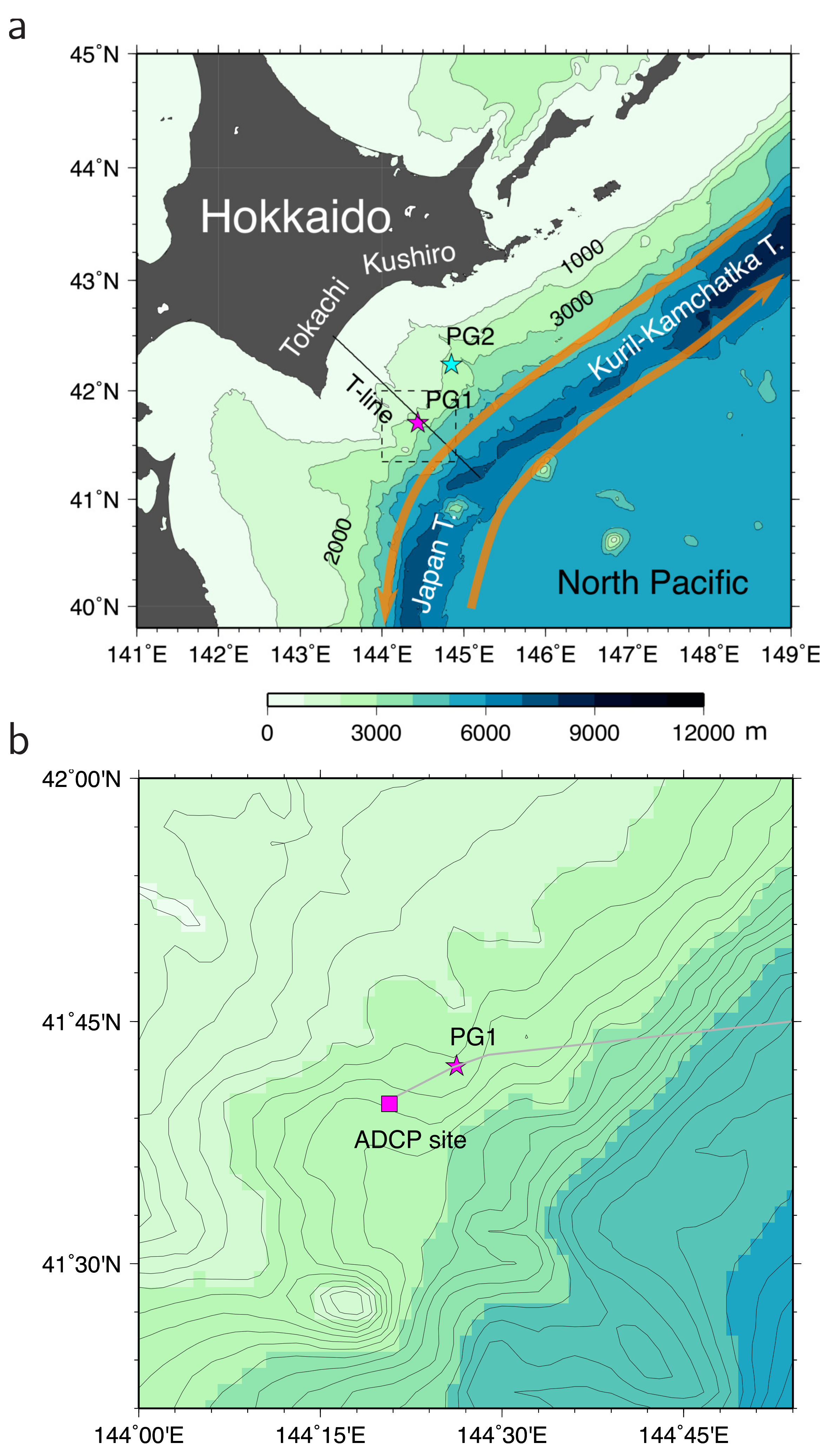
Figure 1.
(a) Locations of the ADCP and bottom pressure gauge station PG1 (magenta star) and bottom pressure gauge station PG2 (cyan star) with sea bottom topography. Deep circulation currents are schematically illustrated by orange lines. Coastal-trapped wave (CTW) modes were computed using the topographic data at the southeastward-trending black line (called the T-line). The bottom topography contour interval is 1000 m. (b) Enlarged map of the region around PG1 (magenta star), enclosed by the dashed square in panel (a) and location of the ADCP site (magenta square). The bottom topography contour interval is 200 m. Part of the cable connecting the portable observation system (cable end station) to the land station via PG1 and PG2 is illustrated by gray line.
From the bottom pressure data alone, however, we cannot infer the vertical structure of the disturbances in the deep and bottom layers. Similarly, the single layer measurements of current velocity by current meters cannot deliver vertical current structure. Thus, variations in the current velocity structures just above the seafloor surface, even on timescales longer than the inertial period, have not been sufficiently observed. To elucidate the vertical structure of such long-term variations, we must deploy ADCPs near the bottom pressure gauge to obtain current velocity profiles in long term.
On the seabed, near the bottom pressure gauge at PG1, a portable observation system (cable end station) has been installed (Figure 1b). This system comprises of an ADCP, hydrophone, video camera, and other components and is connected to the battery pack [16]. A cable, connecting the system to a land station, transmits the collected data to land. Consequently, we were able to record an approximately 15-year-long ADCP velocity time series, which is exceptionally long and able to cover the ENSO-scale temporal variations. As described below, we obtained a reasonable time series of the current velocity vectors, ranging from near bottom depth to a height of 388 m, and found a bottom-intensified current. Such a persistent bottom-intensified current has not been documented by past investigators. Furthermore, the northward component of the bottom-intensified current was found to thicken on an interannual timescale; using an ocean general circulation model (OGCM) dataset, we also found that the current travels along the onshore continental slope region of the Japan and Kuril–Kamchatka trenches.
In theory, the current velocity variations over continental slopes cannot be represented by the baroclinic Rossby wave modes, estimated with assumption of a flat bottom ocean, as done by Nagano and Wakita [17] in a study of variations at station K2 in the interior region of the North Pacific subarctic gyre. Fluctuations over the continental slopes are substantially affected by the topography, besides density stratification, being trapped by the continental slopes on subinertial (low) frequencies. These types of waves are called coastal-trapped waves (CTWs) [18,19,20]. The ENSO (i.e., interannual) timescale variation imposed on the southeastern coast of Hokkaido is thought to excite the CTW mode variations over the continental slope.
In this study, by using a rotary empirical orthogonal function (EOF) analysis [21,22,23], we examined the characteristics of the interannual variation of the bottom-intensified current. In addition, we calculated the CTW modes by using the method of Brink and Chapman [24] and demonstrated that the observed current velocity variations can be expressed as a superposition of the CTW modes. The disturbances from the offshore region, which follow excitation by ENSO-related changes in the Aleutian Low, were found to be modified by the bottom slope, off the southeastern coast of Hokkaido. The result is a change in the bottom-intensified current thickness by excitation of the bottom-trapped modes of CTW.
2. Observation and Data
2.1. ADCP Observation
Beginning in July 1999, the Japan Agency for Marine-Earth and Technology (JAMSTEC) created the Long-Term Deep Sea Floor Observatory, off Kushiro–Tokachi in the Kuril Trench. Initiation of this project involved deploying bottom pressure gauges at PG1 and PG2, along with a portable observation system, on which the 150-kHz BBADCP (RD Instruments, Poway, CA, USA) was installed upward on the seabed, at a depth of 2630 m, located at 41°39.909′ N, 144°20.695′ E, approximately 6.7 km southwest of PG1 (Figure 1b) [16,25]. The ADCP was set to collect data every 30 min, at 48 levels, with a depth bin size of 8 m. The entire observation system has continued to collect time series data of current velocity profiles near PG1 and bottom pressure data at PG1 and PG2. The ADCP data are available from January 2001. As described below, because the distance between the ADCP station and bottom pressure gauge station PG1 (~6.7 km) is smaller than the estimated spatial scale of current variation across the continental slope, we refer to the ADCP station as PG1. The data, and detailed accompanying information, are publicly available on the website of the JAMSTEC Submarine Cable Data Center (http://www.jamstec.go.jp/scdc/top_e.html, accessed on 10 February 2022).
We corrected the current directions using the annual difference between true north and geomagnetic north, on the basis of the 12th generation of the International Geomagnetic Reference Field [26]. The data were interpolated onto grids at intervals of 8 m, from 2242 to 2618 m depths. The nominal accuracy of the ADCP data is 1% of the velocity, or (Teledyne RD Instruments). The accuracy was for the observations reported here because the observed range of current speeds was less than 10 . In this study, we calculated monthly mean values. Therefore, the random error is less than by monthly averaging. To examine the interannual variation in current velocity, we further smoothed the data by a 15-month running mean filter.
2.2. OGCM for the Earth Simulator (OFES) Data
We used the current velocity data computed by a global OGCM, which is tuned for the the Earth Simulator (JAMSTEC), based on the Modular Ocean Model, version 3, of the National Oceanic and Atmospheric Administration/Geophysical Fluid Dynamics Laboratory [27]. This model is referred to as the OFES [28,29,30,31]. The OGCM dataset used in this study features horizontal grids of and 54 vertical grids and is driven by sea-surface momentum, heat, and freshwater flux data, provided by the US National Centers for Environmental Prediction/National Center for Atmospheric Research (NCEP/NCAR) [32].
2.3. North Pacific Index
The North Pacific Index (NPI), which is defined as the area-weighted sea-level pressure in the region of N– N, E– W, is an indicator of the strength of the Aleutian Low [33]. During El Niño (La Niña) winters, the Aleutian Low becomes stronger (weaker) via atmospheric teleconnection, e.g., [34]. The NPI anomaly was calculated from the seasonal mean. To focus on the ENSO-timescale variation, smoothing was performed for the NPI anomaly using a 15-month running mean filter. Furthermore, we inverted the sign of the NPI anomaly and used the inverted values. Positive (negative) values of the inverted NPI anomaly indicate strengthening (weakening) of the Aleutian Low, principally due to El Niño (La Niña).
3. Results and Discussion
3.1. Vertical Structure of the Bottom Current
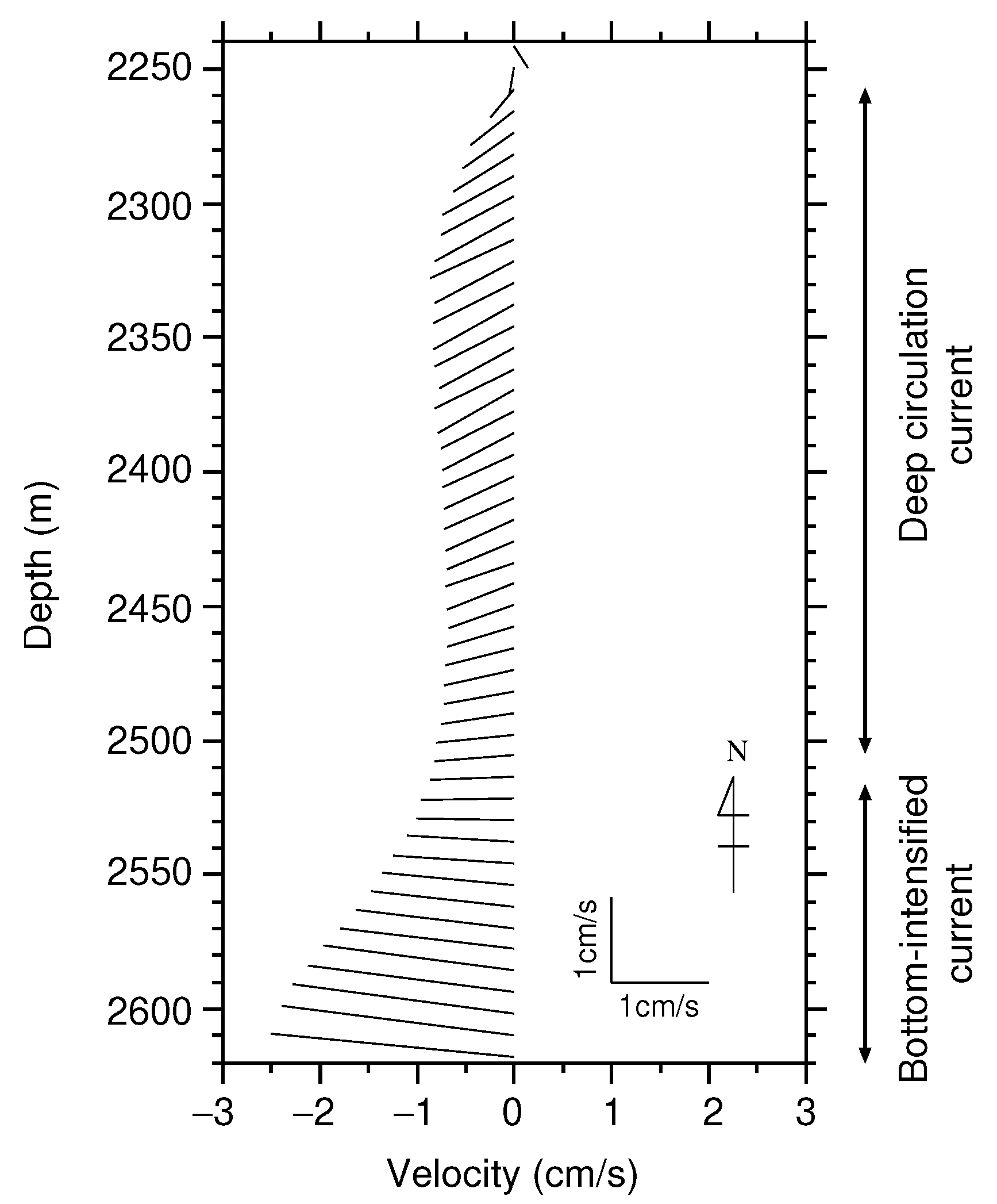
Figure 2a,b show eastward and northward components of the current velocity in a bottom layer, from 2240- to 2620-m depth, as observed by the ADCP at PG1. A southwestward flow was observed down to a depth of approximately 2500 m. This current is part of the deep circulation current flowing southward and southwestward along the northwest and west flank of the Kuril–Kamchatka, Japan, and Izu-Ogasawara trenches, studied by past investigators [35,36,37,38]. Beneath the deep circulation current, we found the bottom current lies at depths between approximately 2500 and 2620 m, which is mostly directed to the west, i.e., toward the shore, and intensifies with depth. This bottom-current structure was more clearly illustrated by averaging within the study period (Figure 3). The lower end of the deep circulation current was present at a height of approximately 110 m above the seabed. The underlying bottom current reached speeds of just above the seabed and is along an isopleth of 2600 m (Figure 1b). Such a bottom-intensified current has not been revealed by geostrophic velocity calculation, based on snapshot hydrographic observations and vertically sparse moored current meter observations. Similar bottom-intensified currents have been reported, on the basis of snapshot observations from lowered ADCPs on the continental slope off the south coast of Shikoku [9].
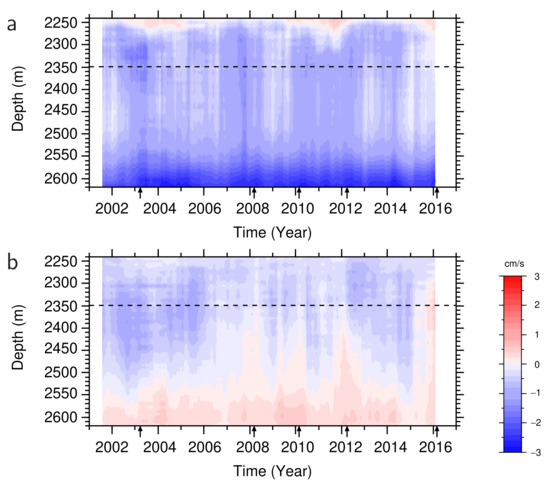
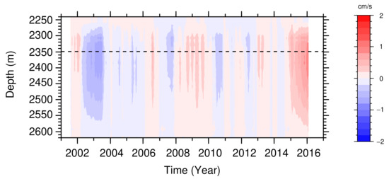
Figure 2.
Time-depth diagrams of the (a) eastward and (b) northward components of the acoustic Doppler current profiler (ADCP) current velocity (), within a depth range from near the ocean bottom to 2240 m at station PG1. Smoothing was performed by a 15-month running mean filter to eliminate variations on timescales shorter than 1 year. Horizontal dashed lines indicate the 2349 m depth level, for which the current velocity fields, produced by the OFES, are illustrated in Figure 4. Arrows mark the periods for which the OFES current velocity fields are shown in Figure 4.
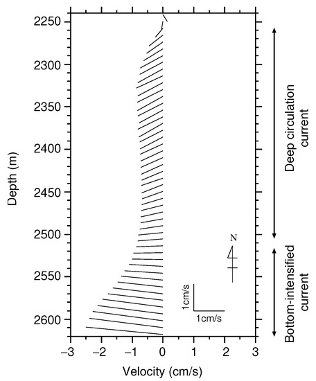
Figure 3.
Mean profile of the ADCP current velocity vector at PG1. Mean values were calculated using the data collected from 2001 to 2016.
The thickness of the bottom-intensified current (>50 m) at PG1 is greater than that of the bottom Ekman layer, which is roughly estimated to be 20 m at most, according to the formula used by Wimbush and Munk [39] and others. There is a topographic depression of approximately 600 m to the south of the ADCP site (Figure 1b). A cyclonic eddy is anticipated to be trapped within the topographic depression. If this anticipation is correct, the trapped cyclonic eddy would intensify the current at the ADCP site. Then, the top of the cyclonic eddy should be shallower than the ADCP site (2630 m) and deeper than the 2400 m isopleth. In observation, the top of the bottom-intensified current is within the depth range. These findings suggest that the bottom-intensified current can be attributed to the local topography that impedes the mean southwestward deep current (Figure 1), rather than a result of turbulent diffusion.
Furthermore, as clearly shown in Figure 2b, the northward component of the bottom-intensified current extended upward, reaching a level shallower than 2400 m depth on an interannual timescale, as in the winters of 2007/2008, 2009/2010, 2011/2012, and 2015/2016. During the study period, the current thickness varied within a range from approximately 50 m during the 2002/2003 winter to 350 m during the 2015/2016 winter. For example, the OFES current velocity fields at a depth of 2349 m (horizontal dashed lines in Figure 2), in periods marked by arrows in Figure 2, are shown in Figure 4. The diminished bottom-intensified current in March 2003 had no single continuous current along the trenches (Figure 4a). Except for March 2008, the extended bottom-intensified current featured a narrow (~50 km) northward and northeastward current, exceeding , along the Japan and Kuril–Kamchatka trenches (Figure 4c,d). In March 2008 (Figure 4b), the bottom current was vertically extended but the current speed produced by the OFES was quite low. Accordingly, this suggests that the bottom-intensified current frequently becomes elongated and trapped along the onshore continental slope of the trenches, in association with upward extension. However, we note that the OFES does not produce quantitatively accurate velocity and may not be able to sufficiently resolve the cross-shelf structure of the bottom-intensified current. The mechanism of the vertical extension of the current will be discussed in Section 3.3.
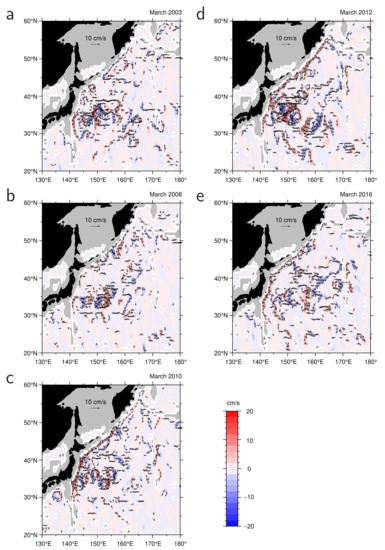
Figure 4.
OFES current velocity vector (arrows) and northward velocity component (color gradient) fields at a depth of 2349 m in (a) March 2003, (b) March 2008, (c) March 2010, (d) March 2012, and (e) March 2016, which are marked by the arrows in Figure 2b. Panel (a) shows the current vector field in period of vertically shrunken state of the bottom-intensified current at PG1, and other panels display the current fields in periods of vertically extended states of the current. Velocity vectors with speeds lower than 3.0 are not shown.
3.2. The Rotary EOF Modes of the Bottom Current Variation
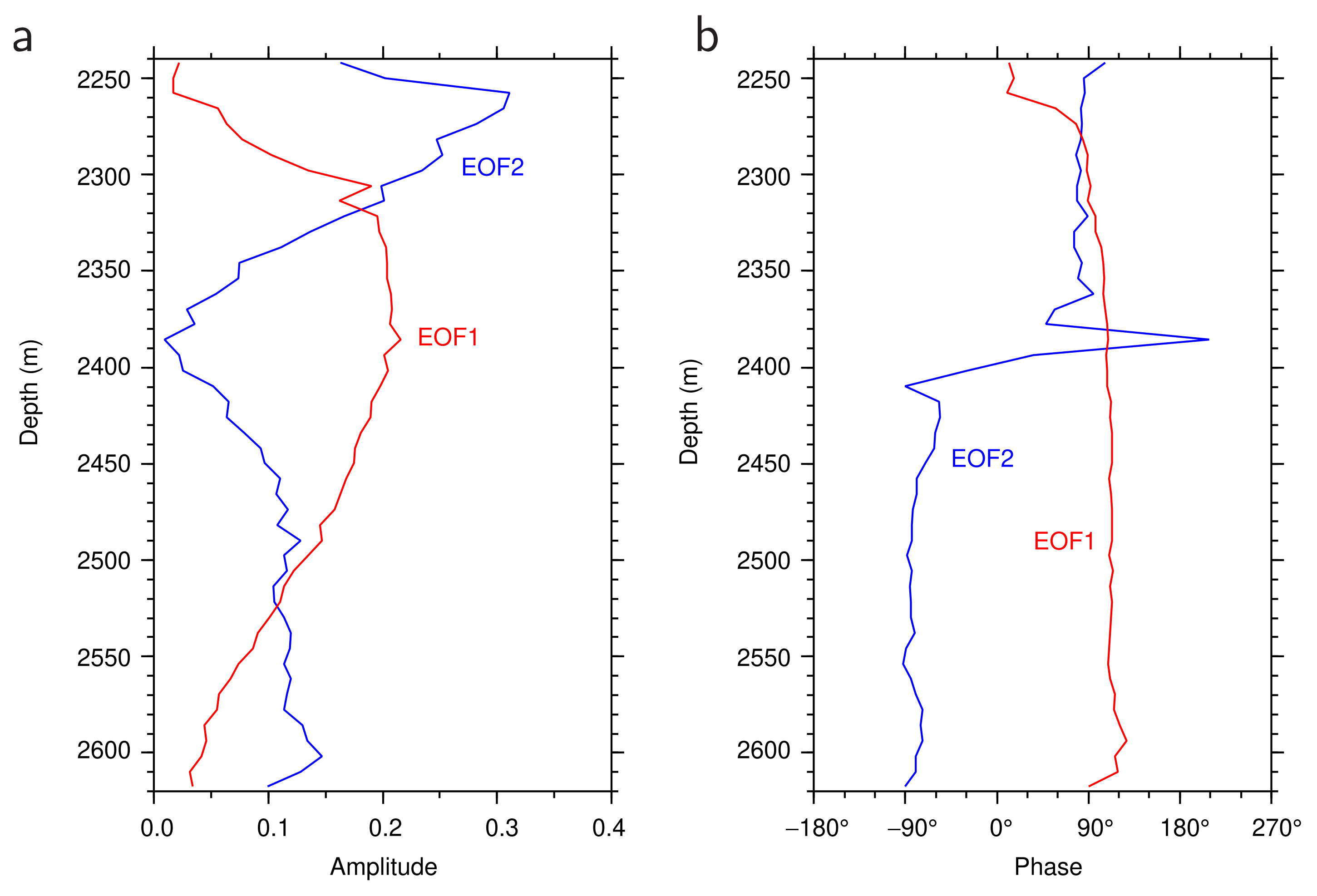
To examine variations in the bottom-intensified current, we decomposed the variation in the ADCP-observed current velocity vector at PG1 by rotary EOF modes (Figure 5). The percentages of the first and second rotary EOF modes are 76% and 14%, respectively. These two rotary EOF modes explain approximately 90% of the total variance in the monthly current velocity variation. The first rotary EOF mode, i.e., the dominant mode variation, has a maximum amplitude at a depth of 2380 m (red line in Figure 5a). The upward extension of the bottom-intensified current is principally attributable to the first rotary EOF mode. As the phase of the first rotary EOF mode has a nearly constant value of approximately , except in the uppermost observed layer (blue line), in which the amplitude is quite small, the first mode variation is directed along the continental slope. The second rotary EOF mode changes the phase between depths of approximately 2380 and 2410 m (blue line in Figure 5b), representing current velocity variations with smaller vertical scales than the first mode variation.

Figure 5.
(a) Amplitudes and (b) phases of the first (red lines) and second (blue lines) rotary EOF modes of the ADCP current velocity at PG1, with respect to depth. In panel (b), counterclockwise rotation was set to correspond to the positive phase.
The time coefficient of the first rotary EOF mode exhibits interannual variation, with significant positive peaks in the winters of 2002/2003, 2007/2008, 2009/2010, 2011/2012, and 2015/2016 (Figure 6a). Most of these positive peaks lag behind the positive peaks of the inverted NPI anomaly (gray line), which represent the strengthening of the Aleutian Low, principally due to the occurrence of El Niño events, e.g., [34]. With a lag of 3 months, the correlation coefficient between the first rotary EOF mode and inverted NPI anomaly reaches a maximum of , which is higher than the 99% confidence limit () and, therefore, statistically significant. The time-lag is unexpectedly shorter than the time lag (30 months) between the sea surface height variation at PG1 and inverted NPI anomaly, calculated by Hasegawa et al. [14]. This very short time lag suggests that the vertical extension of the bottom-intensified current is brought about by a barotropic response in the central Pacific to ENSO-related wind variation, which is relatively rapid, in comparison to the baroclinic response [17].
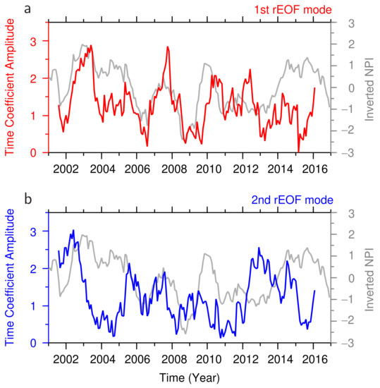
Figure 6.
Amplitudes of time coefficients of the (a) first (red line) and (b) second (blue line) rotary EOF modes of the ADCP current velocity at PG1, as well as the inverted North Pacific Index (NPI) anomaly (gray line). The time coefficients and inverted NPI anomaly were normalized by the standard deviations.
The current velocity actually observed is related to the phase of the time coefficient of the first rotary EOF mode (not shown), besides the amplitude. For this reason, the positive peaks of the time coefficients (Figure 6a) do not always coincide with the upward extensions of the bottom-intensified current (Figure 2b). In Figure 7, we show the current velocity variation along the continental slope (or perpendicular to the T-line in Figure 1), constructed from the first rotary EOF mode. The first rotary EOF mode current velocity variation exhibits positive peaks that correspond to the vertical extensions of the bottom-intensified current in 2007/2008, 2009/2010, 2011/2012, and 2015/2016, as mentioned in Figure 2b. Furthermore, the negative peak of the first mode variation in 2002/2003 concurred with shrinkage of the bottom-intensified current. The correlation coefficient between the second rotary EOF mode (blue line in Figure 6b), and the inverted NPI anomaly is lower than the 99% confidence limit, even if time lags are considered.
The ENSO-related barotropic disturbances that propagated westward in the interior region of the oceans as Rossby waves and impinged on the continental slope were strongly modified by the topography along the western boundary. Thus, we expect that the modified current disturbances over the continental slope to be expressed as a superposition of CTW mode waves.
3.3. Current Structures of Coastal-Trapped Wave Modes
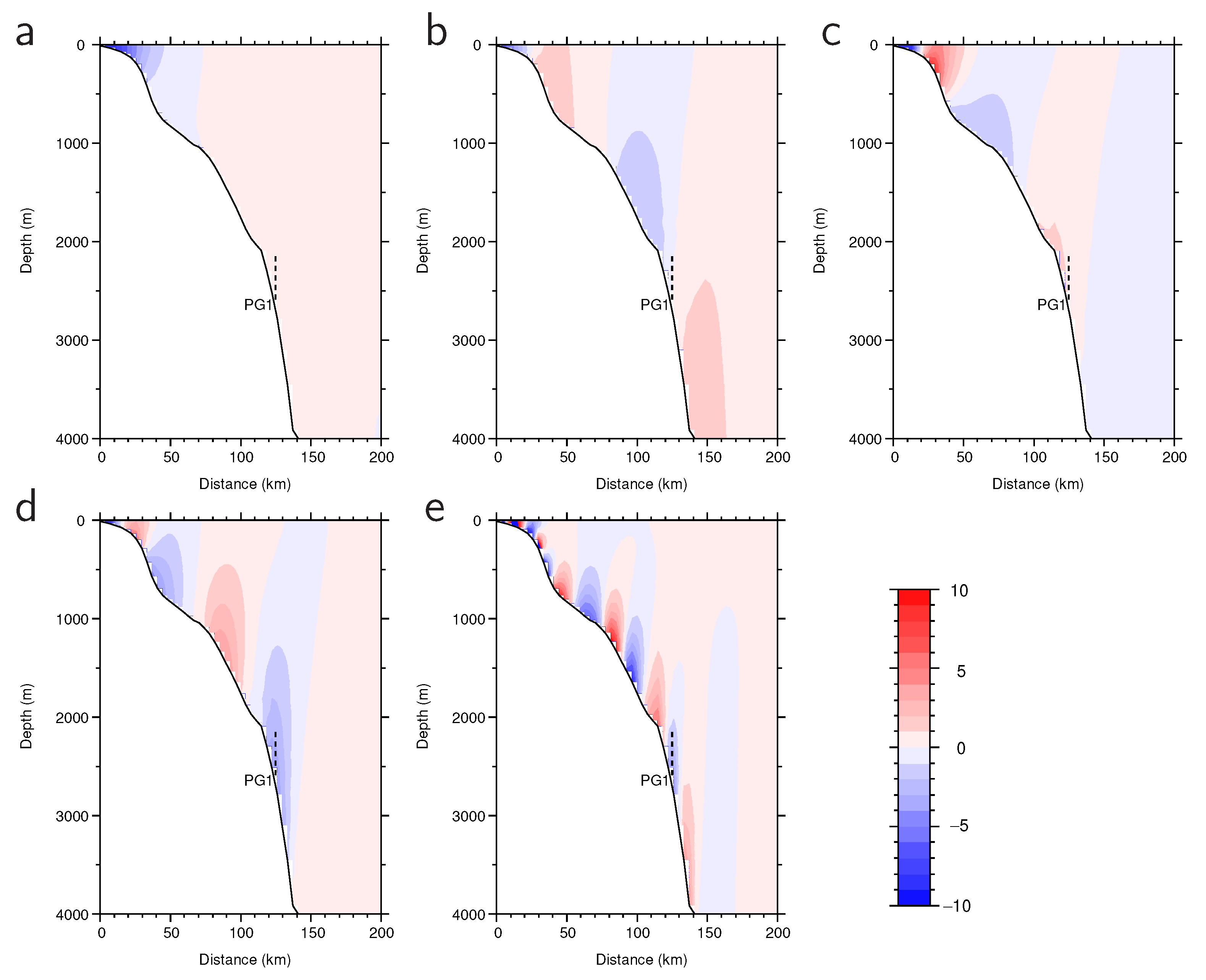
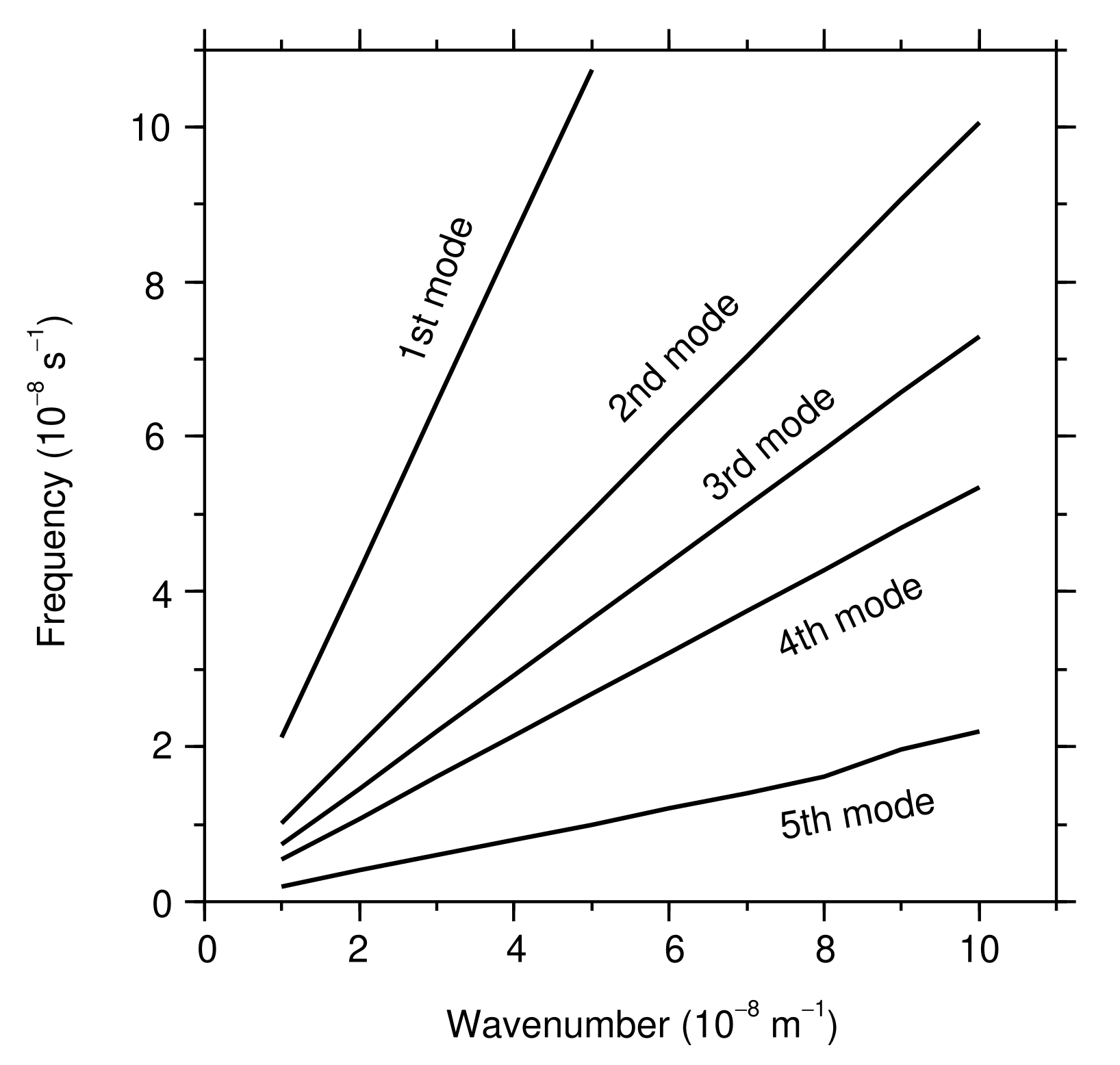
We calculated eigenfunctions of CTW modes from the f-plane linearized hydrostatically balanced equations of motion and continuity for an inviscid fluid, assuming a rigid-lid condition, using the software BIGLOAD4 developed by Brink [40] and Brink and Chapman [24]. For the calculation, we used a horizontally uniform Brunt–Väisälä frequency profile, on the basis of hydrographic data at N, E from the World Ocean Atlas 2018 [41] and ETOPO1 [42] depth data at the T-line. Figure 8 shows the eigenfunctions of the along-slope velocity component for the first to fifth CTW modes. Aside from the first CTW mode, the calculated CTW modes are bottom-trapped. The vertical scale of these modes are mainly attributed to the density stratification. The higher the mode, the smaller the spatial scale tends to be along the T-line. Fixed to the approximate period (reciprocal of frequency) of ENSO (~4 years), the wavelengths of these CTW mode waves were evaluated to be longer than 3 × 10 km (Figure 9). This is considerably longer than the along-trench length of the northward current on the continental slope (~3000 km) produced in the OFES. Although the computation of the CTW modes does not account for dissipation effects, CTW disturbances in the OFES and in the real ocean must be dissipated by friction with the seabed.

Figure 8.
Sections of the eigenfunctions of the along-slope current velocity component for the (a–e) first to fifth coastal-trapped wave (CTW) modes, with a wavenumber of at the T-line in Figure 1. The vertical dashed lines show the vertical range of the ADCP observation at PG1.

Figure 9.
Dispersion relations of the lowest five coastal-trapped wave (CTW) modes at the T-line in Figure 1.
The variations in the along-slope component of the bottom-intensified current are considered to be related to these CTW mode variations. To examine whether or not the observed current velocity variations perpendicular to the T-line are represented as a superposition of the CTW modes, we performed a regression of the observed variations to the five CTW modes. The resultant variations, constructed by the five CTW modes (Figure 10), are remarkably similar to the first rotary EOF mode variation (Figure 7). The correlation coefficients between these time series are higher than for most depth levels. Hence, the observed vertical extension of the along-slope component of the bottom-intensified current can be explained by the excitation of the bottom-trapped (second to fifth) modes of CTW, by impingement of ENSO-related barotropic Rossby wave disturbances on the continental slope off the southeast coast of Hokkaido.

Figure 10.
Time-depth diagram of current velocity variations perpendicular to the T-line (Figure 1) by the lowest five coastal-trapped wave (CTW) modes, fitted to the first rotary EOF mode variation at PG1. The horizontal dashed line indicates the 2349 m depth level, for which the OFES current velocity fields are illustrated in Figure 4.
4. Summary
By using current velocity profile data, collected near PG1 (41°39.909′ N, 144°20.695′ E), from 2001 to 2016, by an upward-looking ADCP installed on the seabed (2630-m depth), we examined changes in the current velocity structure near the ocean bottom on the continental slope off the southeast of Hokkaido, Japan. At the site, the deep circulation current, which has been observed by past investigators, e.g., [37], flows southwestward down to a depth of approximately 2520 m (a height of approximately 110 m above the seabed) on average. In the bottom layer, from approximately 2520- to 2620-m depth, the current speed increases with depth, up to immediately above the seabed.
The thickness of the bottom-intensified current changes on an interannual timescale, within a range of 50–350 m. The OFES current velocity data show that the thickened bottom-intensified current flows northward, trapped along the onshore continental slope of the Japan and Kuril–Kamchatka trenches. The first rotary EOF mode, which accounts for 76% of the total variance of the variation, has a nearly constant phase and a peak amplitude around 2380 m depth. The first rotary EOF mode becomes enhanced (or attenuated) 3 months after the strengthening (or weakening) of the Aleutian Low, forced by the El Niño (La Niña) teleconnection. The current velocity variation along the continental slope, due to the first rotary EOF mode, represents the interannual change in the bottom-intensified current thickness.
Except for the first CTW mode, the eigenfunctions (i.e., cross-sectional structure of the along-slope current variation) of the CTW modes on the continental slope off the southeastern coast of Hokkaido are bottom-intensified. The thickness change of the bottom-intensified current is represented as the superposition of the first to fifth CTW modes, particularly of the (second to fifth) bottom-trapped modes of CTW. Hence, the observed interannual thickness changes in the bottom-intensified current are caused by oceanic barotropic disturbances, excited by changes in the Aleutian Low in the central Pacific and modified by the continental slope off the southeast coast of Hokkaido. These results are beneficial for oceanographic studies and ocean engineering, such as suspended sediment studies, the construction and maintenance of marine structures, and the planning of deep drilling.
Author Contributions
Conceptualization, A.N.; formal analysis, A.N. and T.H.; writing—original draft preparation, A.N.; writing—review and editing, T.H., K.A. and H.M.; project administration, K.A.; funding acquisition, A.N., K.A. and T.H. All authors have read and agreed to the published version of the manuscript.
Funding
This work was partly supported by the Japan Society for the Promotion of Science, Grant-in-Aid for Scientific Research (Grant Numbers: JP15H04228, JP16H06473, JP17K05660, JP18H03726, JP19H05702, JP20K04072, JP20H02236, and JP20H04349).
Institutional Review Board Statement
Not applicable.
Informed Consent Statement
Not applicable.
Data Availability Statement
ADCP data are available on the website of the JAMSTEC project “Long-Term Deep Sea Floor Observatory off Kushiro-Tokachi in the Kuril Trench” (http://www.jamstec.go.jp/scdc/top_e.html, accessed on 10 February 2022. OFES data were provided by the Asia-Pacific Data-Research Center of the International Pacific Research Center, the University of Hawaii (http://apdrc.soest.hawaii.edu/index.php, accessed on 10 February 2022). World Ocean Atlas 2018 and ETOPO1 data are published on the websites of National Centers for Environmental Information, National Oceanic and Atmospheric Administration (https://www.ncei.noaa.gov/products/world-ocean-atlas, accessed on 10 February 2022 and https://www.ngdc.noaa.gov/mgg/global/, accessed on 10 February 2022).
Acknowledgments
The authors thank the individuals concerned in the establishment of the JAMSTEC Long-Term Deep Sea Floor Observatory, off Kushiro-Tokachi in the Kuril Trench. The OFES simulation was conducted on the Earth Simulator, under the support of JAMSTEC. The authors express gratitude to Kyoko Taniguchi (JAMSTEC) for correcting the manuscript. Additionally, the authors thank the guest editors (Joseph J. Kuehl and Morgan Xiang) for inviting us to the present special session, as well as the anonymous reviewers for helpful comments.
Conflicts of Interest
The authors declare no conflict of interest.
Abbreviations
The following abbreviations are used in this manuscript:
| ADCP | Acoustic Doppler current profiler |
| CTW | Coastal-trapped wave |
| ENSO | El Niño–Southern Oscillation |
| EOF | Empirical orthogonal function |
| JAMSTEC | Japan Agency for Marine-Earth and Technology |
| NPI | North Pacific Index |
| OFES | Ocean general circulation model for the Earth Simulator |
| OGCM | Ocean general circulation model |
References
- McCane, I.N. Local and Global Aspects of the Bottom Nepheloid Layers in the World Ocean. Neth. J. Sea Res. 1986, 20, 167–181. [Google Scholar] [CrossRef]
- Bomberg, J.; Ariyoshi, K.; Hautala, S.; Johnson, H.P. The Finicky Nature of Earthquake Shaking-triggered Submarine Sediment Slope Failures and Sediment Gravity Flows. J. Geophys. Res. 2021, 126, e2021JB022588. [Google Scholar] [CrossRef]
- Komaki, K.; Nagano, A. Monitoring the deep western boundary current in the western North Pacific by echo intensity measured with lowered acoustic Doppler current profiler. Mar. Geophys. Res. 2019, 40, 515–523. [Google Scholar] [CrossRef]
- Mao, L.; Zeng, S.; Liu, Q.; Wang, G.; He, Y. Dynamical mechanics behavior and safety analysis of deep water riser considering the normal drilling condition and hang-off condition. Ocean Eng. 2020, 199, 106996. [Google Scholar] [CrossRef]
- Williamson, C.H.K.; Govardhan, R. Vortex-induced Vibrations. Annu. Rev. Fluid Mech. 2004, 36, 413–455. [Google Scholar] [CrossRef] [Green Version]
- Davidson, P.A. Turbulence: An Introduction for Scienctist and Engineers, 2nd ed.; Oxford University Press: Oxford, UK, 2015. [Google Scholar]
- Kawabe, M.; Fujio, S.; Yanagimoto, D.; Tanaka, K. Water masses and currents of deep circulation southwest of the Shatsky Rise in the western North Pacific. Deep-Sea Res. I 2009, 56, 1675–1687. [Google Scholar] [CrossRef]
- Komaki, K.; Kawabe, M. Deep-circulation current through the Main Gap of the Emperor Seamounts Chain in the North Pacific. Deep-Sea Res. I 2009, 56, 305–313. [Google Scholar] [CrossRef]
- Nagano, A.; Ichikawa, H.; Ichikawa, K.; Konda, M. Bottom Currents on the continental slope off Shikoku. In Proceedings of the OCEANS 2008—MTS/IEEE Kobe Techno-Ocean, Kobe, Japan, 8–11 April 2008; pp. 1–4. [Google Scholar] [CrossRef]
- Nagano, A.; Ichikawa, K.; Ichikawa, H.; Yoshikawa, Y.; Murakami, K. Large ageostrophic currents in the abyssal layer southeast of Kyushu, Japan, by direct measurement of LADCP. J. Oceanogr. 2013, 69, 259–268. [Google Scholar] [CrossRef]
- Kawabe, M.; Yanagimoto, D.; Kitagawa, S. Variations of deep western boundary currents in the Melanesian Basin in the western North Pacific. Deep-Sea Res. I 2006, 53, 942–959. [Google Scholar] [CrossRef]
- Taira, K.; Teramoto, T. Bottom Currents in Nankai Trough and Sagami Trough. J. Oceanogr. Soc. Jpn. 1985, 41, 388–398. [Google Scholar] [CrossRef]
- Weatherly, G.L.; Kelly, E.A., Jr. Storms and flow reversals at the HEBBLE site. Mar. Geol. 1985, 66, 205–218. [Google Scholar] [CrossRef]
- Hasegawa, T.; Nagano, A.; Matsumoto, H.; Ariyoshi, K.; Wakita, M. El Niño-related sea surface elevation and ocean bottom pressure enhancement associated with the retreat of the Oyashio southeast of Hokkaido, Japan. Mar. Geophys. Res. 2019, 40, 505–512. [Google Scholar] [CrossRef]
- Hasegawa, T.; Nagano, A.; Ariyoshi, K.; Miyama, T.; Matsumoto, H.; Iwase, R.; Wakita, M. Effect of Ocean Fluid Changes on Pressure on the Seafloor: Ocean Assimilation Data Analysis on Warm-core Rings off the Southeastern Coast of Hokkaido, Japan on an Interannual Timescale. Front. Earth Sci. 2021, 9, 600930. [Google Scholar] [CrossRef]
- Hirata, K.; Aoyagi, M.; Mikada, H.; Kawaguchi, K.; Kaiho, Y.; Iwase, R.; Morita, S.; Fujisawa, I.; Sugioka, H.; Mitsuzawa, K.; et al. Real-time geophysical measurements on the deep seafloor using submarine cable in the southern Kurile subduction zone. IEEE J. Ocean Eng. 2002, 27, 170–181. [Google Scholar] [CrossRef]
- Nagano, A.; Wakita, M. Wind-driven decadal sea surface height and main pycnocline depth changes in the western subarctic North Pacific. Prog. Earth Planet. Sci. 2019, 6, 59. [Google Scholar] [CrossRef] [Green Version]
- Gill, A.E.; Clarke, A.J. Wind-induced upwelling, coastal currents and sea-level changes. Deep-Sea Res. 1974, 21, 325–345. [Google Scholar] [CrossRef]
- Huthnance, J.M. On Coastal Trapped Waves: Analysis and Numerical Calculation by Inverse Iteration. J. Phys. Oceanogr. 1978, 8, 74–92. [Google Scholar] [CrossRef] [Green Version]
- Gill, A.E. Atmosphere-Ocean Dynamics; Academic Press: London, UK, 1982. [Google Scholar]
- Denbo, D.W.; Allen, J.S. Rotary Empirical Orthogonal Function Analysis of Currents near the Oregon Coast. J. Phys. Oceanogr. 1984, 14, 35–46. [Google Scholar] [CrossRef] [Green Version]
- Thomson, R.E.; Emery, W.J. Data Analysis Methods in Physical Oceanography, 3rd ed.; Elsevier: Amsterdam, The Netherlands, 2014. [Google Scholar] [CrossRef]
- Nagano, A.; Wakita, M.; Fujiki, T.; Uchida, H. El Niño-related Vertical Mixing Enhancement under the Winter Mixed Layer at Western Subarctic North Pacific Station K2. J. Geophys. Res. 2021, 126, e2020JC016913. [Google Scholar] [CrossRef]
- Brink, K.H.; Chapman, D.C. Programs for Computing Properties of Coastal-trapped Waves and Wind-driven Motions Over the Continental Shelf and Slope; Technical Report WHOI-87-24; Woods Hole Oceanographic Institution: Woods Hole, MA, USA, 1987; p. 02543. [Google Scholar]
- Kawaguchi, K.; Hirata, K.; Mikada, H.; Kaiho, Y.; Iwase, R. An expendable deep seafloor monitoring system for earthquake and tsunami observation network. In Proceedings of the 2000 MTS/IEEE Conference, Providence, RI, USA, 11–14 September 2000; pp. 1719–1722. [Google Scholar]
- Thèbault, E.; Finlay, C.C.; Beggan, C.D.; Alken, P.; Aubert, J.; Barrois, O.; Bertrand, F.; Bondar, T.; Boness, A.; Brocco, L.; et al. International Geomagnetic Reference Field: The 12th generation. Earth Planets Space 2015, 67, 79. [Google Scholar] [CrossRef]
- Pacanowski, R.C.; Griffies, S.M. MOM 3.0 Manual; Geophysical Fluid Dynamics Laboratory/National Oceanic and Atmospheric Administration: Princeton, NJ, USA, 2000.
- Masumoto, Y.; Sasaki, H.; Kagimoto, T.; Komori, N.; Ishida, A.; Sasai, Y.; Miyama, T.; Motoi, T.; Mitsudera, H.; Takahashi, K.; et al. A five-year-eddy-resolving simulation of the world ocean—Preliminary outcomes of OFES (OGCM for the Earth Simulator). J. Earth Simulator 2004, 1, 35–56. [Google Scholar]
- Sasai, Y.; Ishida, A.; Yamanaka, Y.; Sasaki, H. Chlorofluorocarbons in a global ocean eddy-resolving OGCM: Pathway and formation of Antarctic Bottom Water. Geophys. Res. Lett. 2004, 31, L12305. [Google Scholar] [CrossRef]
- Sasaki, H.; Sasai, Y.; Kawahara, S.; Furuichi, M.; Araki, F.; Ishida, A.; Yamanaka, Y.; Masumoto, Y.; Sakuma, H. A series of eddy-resolving ocean simulations in the world ocean: OFES (OGCM for the Earth Simulator) project. In Proceedings of the Oceans ‘04 MTS/IEEE Techno-Ocean ‘04 (IEEE Cat. No.04CH37600), Kobe, Japan, 9–12 November 2004; Volume 3, pp. 1535–1541. [Google Scholar] [CrossRef]
- Sasaki, H.; Nonaka, M.; Masumoto, Y.; Sasai, Y.; Uehara, H.; Sakuma, H. An eddy-resolving hindcast simulation of the quasi-global ocean from 1950 to 2003 on the Earth Simulator. In High Resolution Numerical Modelling of the Atmosphere and Ocean; Ohfuchi, W., Hamilton, K., Eds.; Springer: New York, NY, USA, 2008; pp. 157–185. [Google Scholar] [CrossRef]
- Kalnay, E.; Kanamitsu, M.; Kistler, R.; Collins, W.; Deaven, D.; Gandin, L.; Iredell, M.; Saha, S.; White, G.; Woollen, J.; et al. The NCEP/NCAR 40-year reanalysis project. Bull. Am. Meteorol. Soc. 1996, 77, 437–471. [Google Scholar] [CrossRef] [Green Version]
- Trenberth, K.E.; Hurrel, J.W. Decadal atmosphere-ocean variations in the Pacific. Clim. Dynam. 1994, 9, 303–319. [Google Scholar] [CrossRef]
- Mezzina, B.; Palmeiro, F.M.; Garcia-Serrano, J.; Bladé, I.; Batté, L. Multi-model assessment of the late-winter stratospheric response to El Niño and La Niña. Clim. Dyn. 2021. [Google Scholar] [CrossRef]
- Hallock, Z.R.; Teague, W.J. Evidence for a North Pacific Deep Western Boundary Current. J. Geophys. Res. 1996, 101, 6617–6624. [Google Scholar] [CrossRef]
- Mitsuzawa, K.; Holloway, G. Characteristics of deep currents along trenches in the northwest Pacific. J. Geophys. Res. 1998, 103, 13085–13092. [Google Scholar] [CrossRef] [Green Version]
- Owens, W.B.; Warren, B.A. Deep circulation in the northwest corner of the Pacific Ocean. Deep-Sea Res. I 2001, 48, 959–993. [Google Scholar] [CrossRef]
- Fujio, S.; Yanagimoto, D. Deep current measurements at 38° N east of Japan. J. Geophys. Res. 2005, 110. [Google Scholar] [CrossRef]
- Wimbush, M.; Munk, W. The benthic boundary layer. In The Sea; Maxwell, A.E., Ed.; John Wiley: New York, NY, USA, 1970; Volume 4, pp. 731–758. [Google Scholar]
- Brink, K.H. A Comparison of Long Coastal Trapped Wave Theory with Observations off Peru. J. Phys. Oceanogr. 1982, 12, 897–913. [Google Scholar] [CrossRef] [Green Version]
- Garcia, H.E.; Boyer, T.P.; Baranova, O.K.; Locarnini, R.A.; Mishonov, A.V.; Grodsky, A.; Paver, C.R.; Weathers, K.W.; Smolyar, I.V.; Reagan, J.R.; et al. World Ocean Atlas 2018: Product Documentation; Ocean Climate Laboratory NCEI/NESDIS/NOAA: Princeton, NJ, USA, 2019.
- Amante, C.; Eakins, B.W. ETOPO1 1 Arc-Minute Global Relief Model: Procedures, Data Sources and Analysis; Technical Report, NESDIS NGDC-24; NOAA: Boulder, CO, USA, 2009.


Publisher’s Note: MDPI stays neutral with regard to jurisdictional claims in published maps and institutional affiliations. |
© 2022 by the authors. Licensee MDPI, Basel, Switzerland. This article is an open access article distributed under the terms and conditions of the Creative Commons Attribution (CC BY) license (https://creativecommons.org/licenses/by/4.0/).