Effects of Numerical Forcing on the Two-Time Correlation of Fluid Velocity Differences in Stationary Isotropic Turbulence

Abstract

In direct numerical simulations (DNS) of homogeneous isotropic turbulence, numerical forcing is needed to achieve statistically stationary velocity fields. The Eulerian two-time correlation tensor of the fluid velocity difference field, $\Delta \mathbf{u}(\mathbf{r},t)=\mathbf{u}(\mathbf{x}+\mathbf{r},t)-\mathbf{u}(\mathbf{x},t)$, characterizes the temporal evolution of turbulent eddies whose sizes scale with separation $r=\left|\mathbf{r}\right|$. In this study, we investigate the effects of two spectral forcing schemes on the temporal decay of the Eulerian two-time correlation of fluid velocity differences $⟨\Delta \mathbf{u}(\mathbf{r},t^{\prime })\Delta \mathbf{u}(\mathbf{r},t)⟩$. Accordingly, DNS of homogeneous isotropic turbulence were performed for two grid sizes, ${128}^3$ and ${512}^3$, corresponding to the Taylor micro-scale Reynolds numbers $R{e}_{\lambda }$$\approx 80$ and 210, respectively. Statistical stationarity was achieved by employing deterministic and stochastic spectral forcing schemes. In the stochastic scheme, one needs to specify the time scale, $T_f$, of the Uhlenbeck–Ornstein (UO) processes that constitute the forcing. We considered four values of the UO time scale ($T_f=T_E/4,T_E,2T_E$, and $4T_E$) for each $R{e}_{\lambda }$, where $T_E$ is the large-eddy time scale obtained from the DNS run with deterministic forcing at the same $R{e}_{\lambda }$. It is seen that the correlations $⟨\Delta \mathbf{u}(\mathbf{r},t^{\prime })\Delta \mathbf{u}(\mathbf{r},t)⟩$ obtained from the deterministic-forcing DNS runs decay more slowly than those from stochastic-forcing DNS runs of all four $T_f$ values. The slower decay of correlations in deterministic DNS runs is more pronounced at larger separations and for higher $R{e}_{\lambda }$.

1. Introduction

In Rani et al. [1] and Dhariwal et al. [2], we presented the development of analytical closure model(s) for the unknown diffusion current in the probability density function (PDF) kinetic equation describing the relative positions ($\mathit{r}$) and relative velocities ($\mathit{U}$) of monodisperse high-Stokes-number particle pairs in isotropic turbulence. We showed that in the limit of the Stokes number is $S{t}_r\gg 1$, and the diffusivity tensor characterizing the diffusion current in the $\mathit{U}$-space is equal to $1/{\tau }_v^2$ multiplied by the time integral of the Lagrangian correlation of the fluid velocity differences along particle pair trajectories. Here, $S{t}_r={\tau }_v/{\tau }_r$ is the particle Stokes number based on the time-scale, ${\tau }_r$, of eddies whose sizes are of the order of pair separation, r, and ${\tau }_v$ is the particle viscous relaxation time. In [1,2], analytical closure of the diffusivity tensor was achieved in two steps.

In the first step, the Lagrangian correlation in the diffusivity tensor was converted into a Eulerian two-time correlation of the fluid velocity differences “seen” by particle pairs whose separations remained essentially constant during timescales of $O\left({\tau }_r\right)$, where ${\tau }_r$ is the turnover time of eddies of size r. The Eulerian two-time correlation $⟨\Delta \mathbf{u}(\mathbf{r},t^{\prime })\Delta \mathbf{u}(\mathbf{r},t)⟩$ can be evaluated using a DNS of the stationary isotropic turbulence. In the second step, the diffusivity tensor was analytically closed by systematically converting the Eulerian two-time correlation of the fluid velocity differences into Eulerian two-point correlations of the fluid velocities, which could then be expressed in terms of the Fourier transforms of the velocity spectrum tensor. The second step gives rise to two analytical diffusivity closures—one in which both pair separation (r) and pair center-of-mass position ($x$) remain fixed during flow integral time scales and the other in which only r remains fixed. The former closure is applicable in the Stokes number regime $S{t}_r\gg 1$ and $S{t}_I\gg 1$. Here $S{t}_I={\tau }_v/{\tau }_I$ is the Stokes number based on the integral time scale, ${\tau }_I$. In the latter, we relax the $S{t}_I\gg 1$ requirement so that this closure is valid for $S{t}_r\gg 1$ and $S{t}_I\lesssim 1$. An important feature of both closures is that they contain a single unique expression for the diffusivity at pair separations spanning the entire spectrum of turbulence scales. This is in contrast to prior closures that involved velocity structure functions with different forms for the integral, inertial subrange, and Kolmogorov-scale separations (e.g., [3,4,5]). Using the latter closure, which is applicable for $S{t}_r\gg 1$ and $S{t}_I\lesssim 1$, Rani et al. [1] and Dhariwal et al. [2] evolved the Langevin equations, which are statistically equivalent to the Fokker–Planck equation, for pair relative velocities and separations in stationary isotropic turbulence.

In Dhariwal et al. [2], we performed a detailed quantitative analysis of the three diffusivity closure forms presented in [1]. Closure form 1 (or CF1) refers to the diffusivity containing the time integral of the Eulerian two-time correlation of fluid velocity differences, i.e., the time integral of $⟨\Delta \mathbf{u}(\mathbf{r},t^{\prime })\Delta \mathbf{u}(\mathbf{r},t)⟩$. In CF1, we directly computed this correlation using DNS of forced isotropic turbulence containing fixed (or stationary) particles and integrated the correlation in time to yield the diffusivity. In closure forms 2 and 3 (CF2 and CF3), we utilized the two diffusivity expressions (containing wavenumber integrations) that were obtained in the second step mentioned above (CF3 being valid for $S{t}_I\lesssim 1$). In both Rani et al. [1] and Dhariwal et al. [2], we presented an elaborate discussion of the comparison of the three closure approximations. Therefore, in the following discussion, we focus primarily on elucidating the background and motivation for the current study.

In Dhariwal et al. [2], an extensive comparative analysis of the three closure forms of diffusivity was undertaken. The diffusivities were quantitatively compared with each other as well as with the theory of Zaichik and Alipchenkov [3] and its refined form [4]. Langevin simulations of pair separations and relative velocities were performed using each of the three closure forms. The statistics of particle-pair relative motion, including the radial distribution function (RDF) and relative velocity moments, obtained from Langevin simulations of the three closures were compared with each other as well as with the DNS data. A key observation of Dhariwal et al. [2] was that closure form 1 (CF1) diffusivity was significantly more sensitive to changes in the Taylor micro-scale Reynolds number, $R{e}_{\lambda }$, than the CF2 and CF3 diffusivities. We found that CF1 diffusivity showed a substantial increase with $R{e}_{\lambda }$ at pair separations $r\gtrsim L$, where L is the integral length scale. In contrast, the closure form 2 (CF2) and closure form 3 (CF3) diffusivities showed only a marginal decrease with $R{e}_{\lambda }$ at these separations.

The enhanced sensitivity of CF1 diffusivity to $R{e}_{\lambda }$ was also manifested in the relative velocity variances of the particle pairs computed from Langevin simulations based on CF1. At higher $R{e}_{\lambda }$, it was observed that the variances obtained using the CF1 diffusivity were significantly higher than the variances computed using DNS as well as those obtained using CF2 and CF3. These trends were particularly pronounced for the smaller Stokes numbers considered in that study. We had hypothesized (without explicit quantitative evidence) that the increase in the CF1 diffusivity with $R{e}_{\lambda }$ may have been an artifact of the deterministic forcing that was used to achieve the statistically stationary velocity fields in the DNS runs. The deterministic forcing involved maintaining the turbulent kinetic energy constant in time by resupplying the energy dissipated during a time step to a narrow wavenumber band at small wavenumbers (or large scales). Our conjecture was that the forcing artificially increased the temporal coherence of the large-scale eddies, particularly as $R{e}_{\lambda }$ increased. The increased coherence led to higher magnitudes of the two-time correlations of the relative fluid velocities (and thereby diffusivities) at separations that scaled with the integral length scale.

The objective of the current study is to quantitatively investigate the above hypothesis. Accordingly, we performed direct numerical simulations of forced isotropic turbulence laden with disperse but fixed particles. Two types of forcing schemes were used to achieve statistical stationarity, namely, the deterministic forcing of Witkowska et al. [6] and the stochastic forcing of Eswaran and Pope [7]. Both [6,7] apply forcing to the low-wavenumber modes in the spectral space. However, forcing may also be applied in physical space as in Lundgren [8] and Petersen and Livescu [9]. Lundgren [8] employed a linear forcing of the form $\mathit{f}=Q\mathit{u}$, where $Q=⟨ϵ⟩/3u^{\prime 2}$ is a constant. Here, $⟨ϵ⟩$ is the mean dissipation rate, and $u^{\prime }$ is the root-mean-square velocity of the turbulence. The principal difference between the Lundgren [8] scheme and those in [6,7] is that the former involves uniformly forcing all wavenumbers, whereas the latter two apply forcing in a narrow range of wavenumbers in the energy-containing range. Subsequently, Petersen and Livescu [9] extended the work of Lundgren [8] to compressible isotropic turbulence, wherein separate solenoidal and dilatational parts of the forcing term are necessary to achieve stationarity. Using DNS of stationary isotropic turbulence, Rosales and Meneveau [10] compared the linear physical-space forcing scheme of Lundgren [8] with the band-limited spectral forcing scheme. Rosales and Meneveau [10] demonstrated that the temporal evolution of the turbulent kinetic energy and energy spectrum computed using the forcing scheme of Lundgren [8] are in good agreement with the corresponding statistics computed from a pseudo-spectral DNS with the band-limited spectral forcing scheme. However, the integral length scale computed using the Lundgren [8] forcing was found to be smaller than that evaluated using the spectral forcing scheme. A consequence of the smaller integral length scale is that for a given $R{e}_{\lambda }$, the grid resolution requirements for the physical forcing are more stringent than for spectral forcing. The other shortcoming of the physical forcing method is that it generates highly oscillatory turbulence statistics, and simulations must be conducted for a significantly longer time in order to attain a statistically stationary state [10].

In the current study, DNS were undertaken for two grid sizes (${128}^3$ and ${512}^3$) using deterministic and stochastic forcing schemes. The Taylor micro-scale Reynolds number, $R{e}_{\lambda }$, was held nearly constant (varying by less than 3%) among the deterministic and stochastic DNS runs for a given grid size. The nominal values of $R{e}_{\lambda }$ were ≈80 and 210 for the ${128}^3$ and ${512}^3$ grids, respectively. When employing the stochastic forcing scheme, we also considered the effects of varying the correlation time scale, $T_f$, of the independent Uhlenbeck–Ornstein (UO) processes that constitute the forcing. We considered four values of $T_f$, ranging from $T_E/4$ to $4T_E$, where $T_E$ is the large-eddy time scale obtained from the DNS run with deterministic forcing for the same grid size. Our motivation for considering this range of $T_f$ values was to study whether the time scale of the stochastic forcing itself had an effect similar to the deterministic forcing on the relative velocity correlations. Using the statistically stationary DNS velocity fields, we computed the Eulerian two-time correlations of the relative fluid velocities seen by fixed particles.

The paper is organized as follows. Section 2.1 presents a brief summary of closure form 1 (CF1) for the diffusivity tensor. Section 2.2 discusses the computational aspects of the direct numerical simulations, including the two types of forcing schemes used in the DNS runs. Section 3 compares the Eulerian two-time correlations of the relative fluid velocities obtained from DNS with deterministic and stochastic forcing schemes. We conclude by summarizing our findings in Section 4.

2. Methodology

2.1. Diffusivity Closure

In Rani et al. [1], we showed that the governing equation for the probability density function (PDF), $\Omega (\mathit{r},\mathit{U})$, of monodisperse particle pairs with Stokes numbers of $S{t}_r\gg 1$ is of the Fokker–Planck form:

$$\begin{array}{c}\hfill \frac{\partial \Omega }{\partial t}+{\mathbf{\nabla }}_{\mathbf{r}}·(\mathit{U}\Omega )-\frac{1}{{\tau }_v}{\mathbf{\nabla }}_{\mathit{U}}·(\mathit{U}\Omega )-{\mathbf{\nabla }}_{\mathit{U}}·({\mathit{D}}_{UU}·{\mathbf{\nabla }}_{\mathit{U}}\Omega )=0\end{array}$$

(1)

where ${\tau }_v$ is the particle viscous relaxation time, $\mathit{r}$ and $\mathit{U}$ are the pair separation and relative velocity vectors, respectively, and ${\mathit{D}}_{UU}$ is the relative-velocity space diffusivity tensor characterizing the diffusion current.

In Closure Form 1 (CF1), which is the focus of the current study, the relative-velocity space diffusivity ${\mathit{D}}_{UU}$ is given by

$$\begin{array}{ccc}\hfill {\mathit{D}}_{UU}^{\left[1\right]}\left(r\right)& =& \frac{1}{{\tau }_v^2}{\int }_{-\infty }^0⟨\Delta \mathit{u}(\mathit{r},\mathit{x},0)\Delta \mathit{u}(\mathit{r},\mathit{x},t)⟩dt\hfill \end{array}$$

(2)

where the integrand is the Eulerian two-time correlation of the relative fluid velocities with both the pair separation, $\mathit{r}$, and pair center-of-mass position, $\mathit{x}$, held fixed. The relative fluid velocity (or the fluid velocity difference), $\Delta \mathit{u}(\mathit{r},\mathit{x},t)$, is given as

$$\Delta \mathit{u}(\mathit{r},\mathit{x},t)=\mathit{u}(\mathit{x}+\frac{\mathit{r}}{2},t)-\mathit{u}(\mathit{x}-\frac{\mathit{r}}{2},t)$$

(3)

For isotropic turbulence, we can write the ${\mathit{D}}_{UU}$ tensor as

$${\mathit{D}}_{UU,ij}={\mathit{D}}_{UU,\perp }\left({\delta }_{ij}-\frac{r_i{r}_j}{r^2}\right)+{\mathit{D}}_{UU,\left|\right|}\frac{r_i{r}_j}{r^2}$$

(4)

where ${\mathit{D}}_{UU,\perp }$ and ${\mathit{D}}_{UU,\left|\right|}$ represent the transverse and longitudinal components of ${\mathit{D}}_{UU}$. In Dhariwal et al. [2], ${\mathit{D}}_{UU}^{\left[1\right]}$ was evaluated by computing the transverse and longitudinal components of the two-time correlation $⟨\Delta \mathit{u}(\mathit{r},\mathit{x},0)\Delta \mathit{u}(\mathit{r},\mathit{x},t)⟩$ from DNS of forced isotropic turbulence with fixed particles and then integrating these in time.

2.2. Computational Details of DNS

Direct numerical simulations (DNS) of forced isotropic turbulence are performed on a three-dimensional (3-D) periodic cubic box of length $2\pi$ using a pseudospectral method. The 3-D computational domain is discretized into $N^3$ grid points, with N equally spaced mesh points in each spatial direction. A detailed description of the pseudospectral algorithm used in this study can be found in [11,12].

The fluid velocity, $\mathit{u}$, is computed numerically by solving the governing Navier–Stokes and continuity equations:

$$\begin{array}{c}\frac{\partial \mathit{u}}{\partial t}=-\mathit{\omega }\times \mathit{u}-\mathbf{\nabla }\left(p/{\rho }_f+{\mathit{u}}^2/2\right)+\nu {\mathbf{\nabla }}^2\mathit{u}+\mathit{f}\end{array}$$

(5)

$$\begin{array}{c}\mathbf{\nabla }·\mathit{u}=0\end{array}$$

(6)

where $\mathit{\omega }=\mathbf{\nabla }\times \mathit{u}$ is the fluid vorticity, p is the pressure, ${\rho }_f$ is the fluid density, and $\mathit{f}$ is the external forcing function applied to achieve a statistically stationary turbulence.

We can transform Equations (5) and (6) into Fourier space and eliminate pressure using the continuity equation to obtain

$$\begin{array}{c}\left(\frac{\partial }{\partial t}+\nu k^2\right)\widehat{\mathit{u}}=-\left(\mathit{I}-\frac{\mathit{k}\mathit{k}}{k^2}\right)·\widehat{\mathit{\omega }\times \mathit{u}}+\widehat{\mathit{f}}\end{array}$$

(7)

where $k^2=\mathit{k}·\mathit{k}$. It is computationally prohibitively expensive to directly evaluate the convolution $\widehat{\mathit{\omega }\times \mathit{u}}$. Therefore, a pseudospectral approach is used where the product of vorticty and velocity ($\mathit{\omega }\times \mathit{u}$) is first computed in physical space and then the result is transformed back into the spectral space. The aliasing errors introduced by the pseudospectral algorithm are eliminated by setting the fluid velocities in spectral space equal to zero for wavenumbers satisfying $k\ge k_{\max }$, where k is the wavenumber magnitude and $k_{\max }=\sqrt{2}\mathrm{N}/3$ is the highest wavenumber magnitude realized in the simulation.

The viscous stress term on the LHS of Equation (7) is handled exactly by multiplying Equation (7) with the integrating factor, $\exp \left(\nu k^{2}t\right)$. This results in the following equation:

$$\frac{\partial }{\partial t}\left[exp\left(\nu k^{2}t\right){\widehat{u}}_i\right]={\mathrm{RHS}}_{i}exp\left(\nu k^{2}t\right),$$

(8)

where ${\mathrm{RHS}}_i=\left(-{\delta }_{im}+\frac{k_i{k}_m}{k^2}\right){ϵ}_{mjk}\mathcal{F}\left\{{\omega }_j{u}_k\right\}$, ${ϵ}_{mjk}\mathcal{F}\left\{{\omega }_j{u}_k\right\}$ represents the convolution $\widehat{\mathit{\omega }\times \mathit{u}}$, and ${ϵ}_{mjk}$ is the Levi–Civita tensor.

The discretization of Equation (8) in time is accomplished using the second-order Runge–Kutta (RK2) algorithm, giving

$${\widehat{u_i}}^{n+1}={\widehat{u_i}}^n\exp \left(-\nu k^{2}t\right)+\left\{{\mathrm{RHS}}_i^n\exp \left(-\nu k^{2}t\right)+{\mathrm{RHS}}_i^{n+1}\right\}$$

(9)

where n is the the previous time-step level and h is the time-step size. To prevent convective instabilities, the time-step size, h, is chosen such that the CFL number $\le 0.5$. Next, a brief discussion of the two types of forcing schemes used in the current study is provided.

2.2.1. Deterministic Forcing

We employed the deterministic forcing scheme developed by Witkowska et al. [6]. In this scheme, the turbulent kinetic energy (TKE) dissipated during a time step is resupplied to the low wavenumbers or large scales of the turbulent kinetic energy spectrum, thus maintaining the TKE constant throughout the simulation. Unlike the stochastic forcing method, no explicit forcing term, $\widehat{\mathit{f}}$, is added to the Navier–Stokes equations. Instead, the fluid velocity components in the forced wavenumber band are scaled to compensate for the energy dissipated during a given time step using the following formula:

$$\widehat{\mathit{u}}(\mathit{\kappa },t+\Delta t)=\widehat{\mathit{u}}(\mathit{\kappa },t+\Delta t)\sqrt{1+\frac{\Delta E_{\mathrm{diss}}(\Delta t)}{{\int }_{{\kappa }_{\min }}^{{\kappa }_{\min }}E(\kappa ,t+\Delta t)d\kappa }}\forall \kappa \in [{\kappa }_{\min },{\kappa }_{\max }]$$

(10)

where $\widehat{\mathit{u}}(\mathit{\kappa },t)$ is the velocity in spectral space, $\Delta E_{\mathrm{diss}}$ is the total kinetic energy dissipated during $\Delta t$, and $E(\kappa ,t+\Delta t)$ is the spectral turbulent kinetic energy in a wavenumber shell with magnitude $\kappa$ at time $t+\Delta t$. In the current study, the velocity components in the range $\kappa \in (0,\sqrt{2})$ were forced using Equation (10).

2.2.2. Stochastic Forcing

The second forcing scheme implemented in this study is the stochastic forcing method of Eswaran and Pope [7]. As opposed to the deterministic forcing, in this method, an explicit forcing term, $\widehat{\mathit{f}}$, is added to Equation (7). The forcing term is non-zero only in the wavenumber band $\kappa \in (0,\sqrt{2})$ and is evolved according to a vector-valued complex Uhlenbeck–Ornstein (UO) process, $\widehat{\mathit{b}}(\mathit{\kappa },t)$, as shown below [13]:

$$\widehat{\mathit{b}}(\mathit{\kappa },t+\Delta t)=\widehat{\mathit{b}}(\mathit{\kappa },t)\left(1-\frac{\Delta t}{T_f}\right)+\mathit{\theta }{\left(\frac{2{\sigma }^2\Delta T}{T_f}\right)}^{1/2}$$

(11)

where $\Delta t$ is the time step, $\mathit{\theta }$ is a vector of complex random numbers whose components are drawn from a standard normal distribution, and ${\sigma }^2$ and $T_f$ are the variance and time-scale, respectively, of the UO process. The stochastic process $\widehat{\mathit{b}}(\kappa ,t)$ has the following properties [7]:

$$\begin{array}{c}⟨\widehat{\mathit{b}}(\mathit{\kappa },t)⟩=0\end{array}$$

(12)

$$\begin{array}{c}⟨\widehat{\mathit{b}}(\mathit{\kappa },t)\widehat{\mathit{b}}*(\mathit{\kappa },t+s)⟩=2{\sigma }^2{\delta }_{ij}\exp (-s/T_f)\end{array}$$

(13)

where an asterisk denotes the complex conjugate. The forcing term, $\widehat{\mathit{f}}$, in Equation (7) is the projection of $\widehat{\mathit{b}}(\mathit{\kappa },t)$ onto the plane normal to $\mathit{\kappa }$:

$$\widehat{\mathit{f}}=\widehat{\mathit{b}}(\mathit{\kappa },t)-\mathit{\kappa }\mathit{\kappa }·\widehat{\mathit{b}}(\mathit{\kappa },t)/(\mathit{\kappa }·\mathit{\kappa })$$

(14)

In order to investigate the effects of the time scale, $T_f$, of stochastic forcing, four values of $T_f$ were considered ($T_f$ = $4T_E$, $2T_E$, $T_E$, and $T_E/4$), where $T_E$ is the large-eddy turnover time obtained from the DNS run with deterministic forcing at the same grid size.

2.3. Relative Velocity Correlation in CF1

Computing the diffusivity, ${\mathit{D}}_{UU}^{\left[1\right]}$, requires the correlation $⟨\Delta \mathit{u}(\mathit{r},\mathit{x},0)\Delta \mathit{u}(\mathit{r},\mathit{x},t)⟩$ as input. This correlation was evaluated using DNS of forced isotropic turbulence with fixed disperse particles. Two simulation parameters that impact the computed correlation are the number of particles (thereby, pairs) and the bin size ($\Delta r$) for pair separations. The bin size refers to the thickness of the radial shell spanning $r-\Delta r/2$ to $r+\Delta r/2$ within which we search for pairs of separation r. An important consideration in determining the number of particles is the need to obtain converged correlations at separations $r\sim \eta$, where $\eta$ is a Kolmogorov length scale. In this regard, we varied the number of particles from ${10}^5$ to ${10}^6$. Although smooth statistics were obtained for $5\times {10}^5$ particles, we used ${10}^6$ particles or ∼$5\times {10}^{11}$ pairs for computing the two-time correlation. The “optimal” bin size for pair separations is determined by balancing two competing requirements: the convergence of statistics at $r\sim \eta$ and the reduction of statistical noise associated an insufficient bin size. We considered bin sizes varying between $\eta /20$ and $2\eta$ and found that a bin size of $\eta /8$ satisfied the two constraints.

Evaluation of the two-time correlation of observed relative fluid velocities for nearly half a trillion pairs is a highly computationally intensive process. We adopted the following procedure to compute these correlations from DNS of isotropic turbulence with fixed particles. Considering two snapshots of the flow separated by a time interval, $\tau$, in a DNS run, the longitudinal and transverse components of the product $\Delta \mathit{u}(\mathit{r},\mathit{x},t)\Delta \mathit{u}(\mathit{r},\mathit{x},t+\tau )$ for a particle pair were stored in the appropriate r bin and then averaged over all pairs within a bin. Next, we averaged the two components over pairs of flow snapshots with the same time separation, $\tau$. For each value of $\tau$, we averaged over 200 such pairs of flow snapshots. The correlations at various separations were then integrated in time to yield the ${\mathit{D}}_{UU}$ for CF1.

3. Results and Discussion

DNS of isotropic turbulence were undertaken using deterministic forcing (DF) and stochastic forcing (SF) for $R{e}_{\lambda }\approx 80$ and 210 at the grid sizes of ${128}^3$ and ${512}^3$, respectively. For each grid size, we performed one DNS run using DF and four DNS runs using SF. The correlation time scale, $T_f$, of the Ornstein–Uhlenbeck processes in the (DNS + SF) simulations were $T_f$ = $4T_E$, $2T_E$, $T_E$, and $T_E/4$, where $T_E$ is the large-eddy turnover time obtained from the (DNS + DF) case at the same $R{e}_{\lambda }$. The four (DNS + SF) cases for a given $R{e}_{\lambda }$ will be referred to as SF1, SF2, SF3, and SF4, in the same order as the aforementioned $T_f$ values. In each DNS run, initially, only the flow field was evolved until statistical stationarity was reached. After stationarity was attained, the flow was seeded at random locations with ${10}^6$ fixed (stationary) particles, and the simulation was started again. During this second stage of the simulation, which lasted for about 15$T_E$, the fluid velocity at each particle location was stored at time intervals of about $2{\tau }_{\eta }$, where ${\tau }_{\eta }$ is the Kolmogorov timescale. After the simulations were complete, the fluid velocities at the particle locations were post-processed to compute the longitudinal and transverse components of the two-time correlation $⟨\Delta \mathit{u}(\mathit{r},\mathit{x},0)\Delta \mathit{u}(\mathit{r},\mathit{x},\tau )⟩$ for various separations of r, as described in Section 2.3.

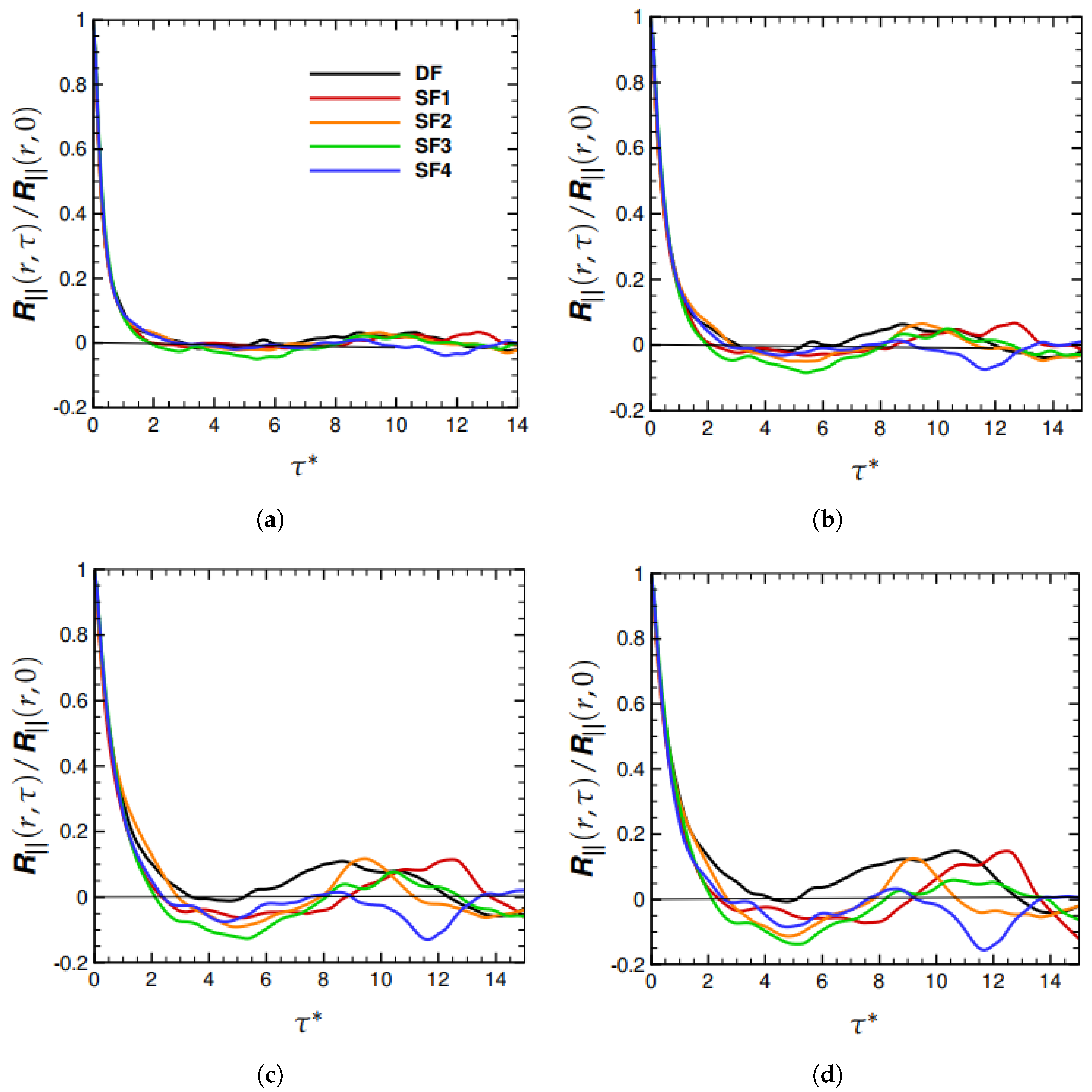
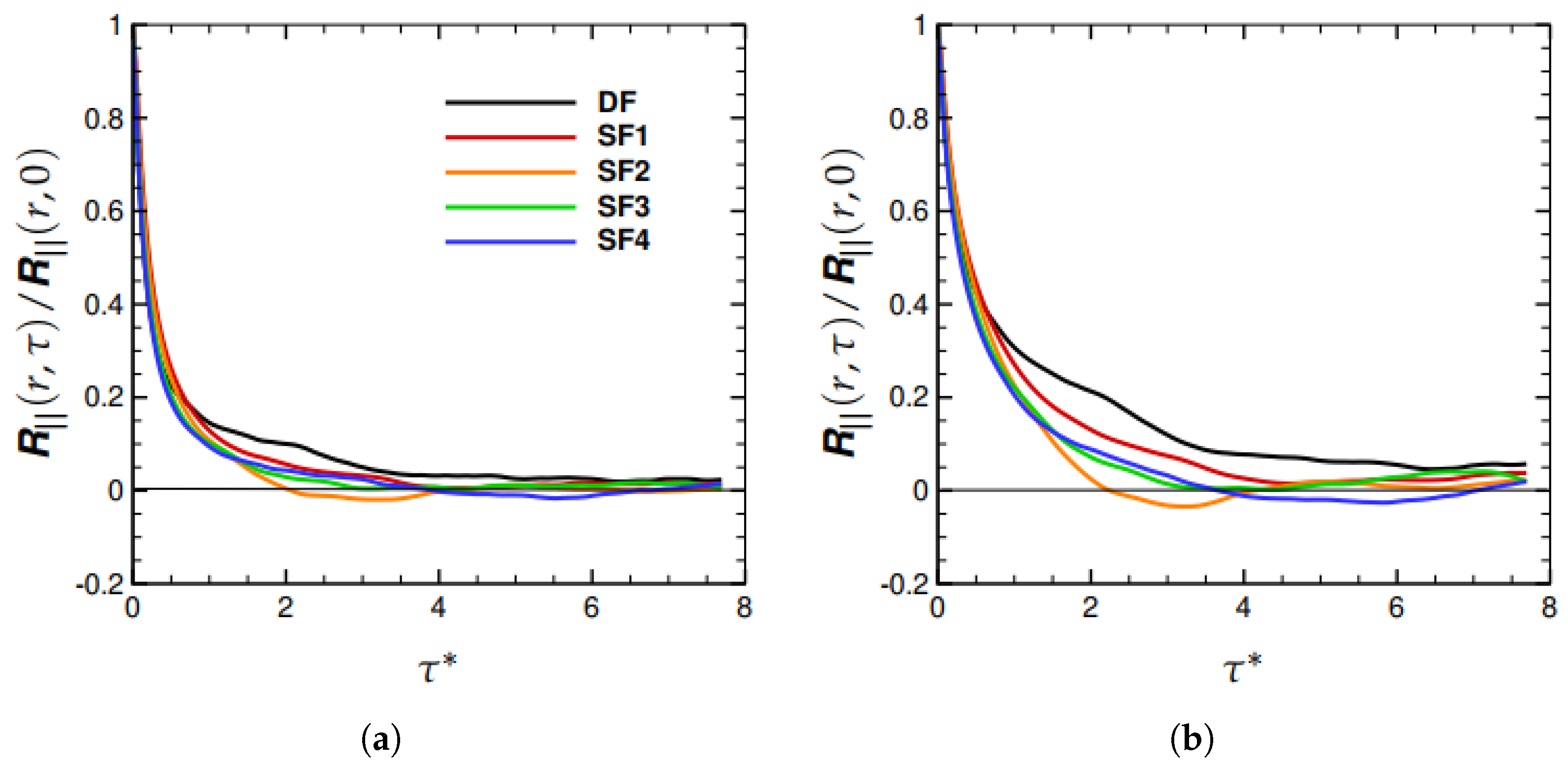
In Figure 1, the longitudinal component of the Eulerian two-time correlation of fluid velocity differences, i.e., ${⟨\Delta \mathit{u}(\mathit{r},\mathit{x},0)\Delta \mathit{u}(\mathit{r},\mathit{x},\tau )⟩}_{\left|\right|}$, is plotted as a function of dimensionless time separation, $\tau *=\tau u_{\mathrm{rms}}/L$ for $R{e}_{\lambda }=80$, where L is the integral length scale and $u_{\mathrm{rms}}$ is the root-mean-square fluctuating velocity. The correlations obtained from the deterministic and stochastic DNS runs were compared at four separations ($r/L=0.56,1.12,2.24$, and $3.36$). In Figure 1a, at $r/L=0.56$, the correlations obtained from the DF and SF runs are in good agreement. For separations $r>L$, the DF correlation progressively increases relative to the SF1–SF4 correlations. At $r/L=1.12$, shown in Figure 1b, the DF correlation exceeds the SF correlations around $\tau *=5$. In Figure 1c,d, for $r/L=2.24$ and $3.36$, respectively, the DF correlation becomes greater than the SF correlations at $\tau *\approx 3$ and $\tau *<2$, respectively. From these trends, it can be deduced that deterministic forcing has the effect of increasing the temporal coherence of eddies larger than the integral length scale, L.

Figure 1. ${\mathit{R}}_{\left|\right|}(r,\tau )={⟨\Delta \mathit{u}(\mathit{r},\mathit{x},0)\Delta \mathit{u}(\mathit{r},\mathit{x},\tau )⟩}_{\left|\right|}$ as a function of dimensionless time separation, $\tau *=\tau u_{\mathrm{rms}}/L$, for $R{e}_{\lambda }=80$. (a) $r/L=0.56$, (b) $r/L=1.12$, (c) $r/L=2.24$, and (d) $r/L=3.36$.

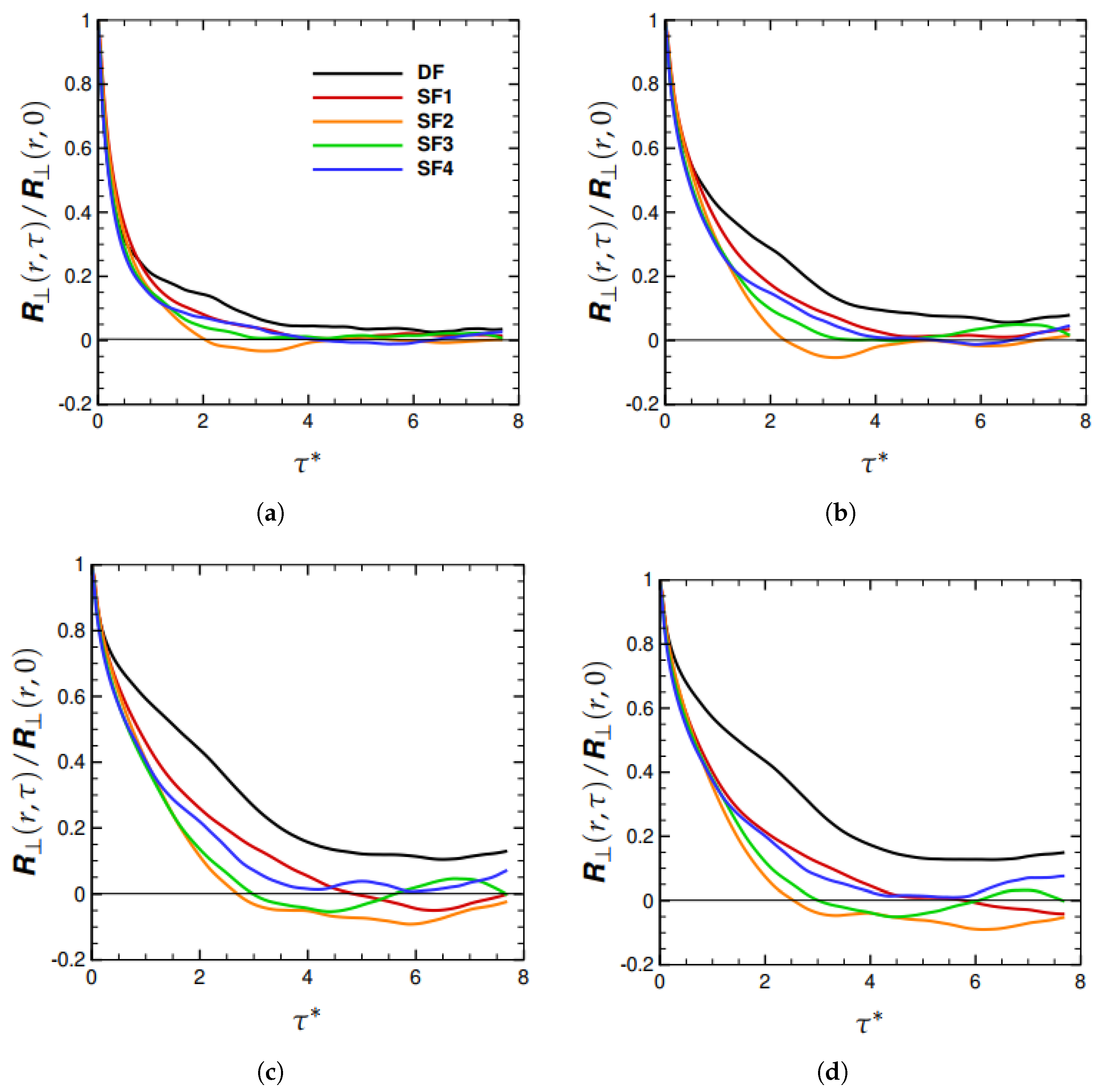
The effects of DF and SF on the the transverse component ${⟨\Delta \mathit{u}(\mathit{r},\mathit{x},0)\Delta \mathit{u}(\mathit{r},\mathit{x},\tau )⟩}_{\perp }$ for $R{e}_{\lambda }=80$ are illustrated in Figure 2a–d. At the smallest separation of $r/L=0.56$, we note that DF has a smaller impact on ${⟨\Delta \mathit{u}(\mathit{r},\mathit{x},0)\Delta \mathit{u}(\mathit{r},\mathit{x},\tau )⟩}_{\perp }$ as compared to that at larger separations. At $r/L=1.12,2.24$, and $3.36$, we see in Figure 2b–d that the $\tau *$ at which the DF correlation exceeds the SF correlations are $\tau *\approx 4$, $\tau *<3$, and $\tau *<1$, respectively, which are all smaller than the corresponding $\tau *$’s in Figure 1. Thus, the transverse component of the two-time correlation shows the effects of DF even more clearly than does the longitudinal component. Furthermore, in Figure 1 and Figure 2, both the longitudinal and transverse correlations for SF1–SF4 do not manifest any clear effects of the variation in the Uhlenbeck–Ornstein time scale, $T_f$.

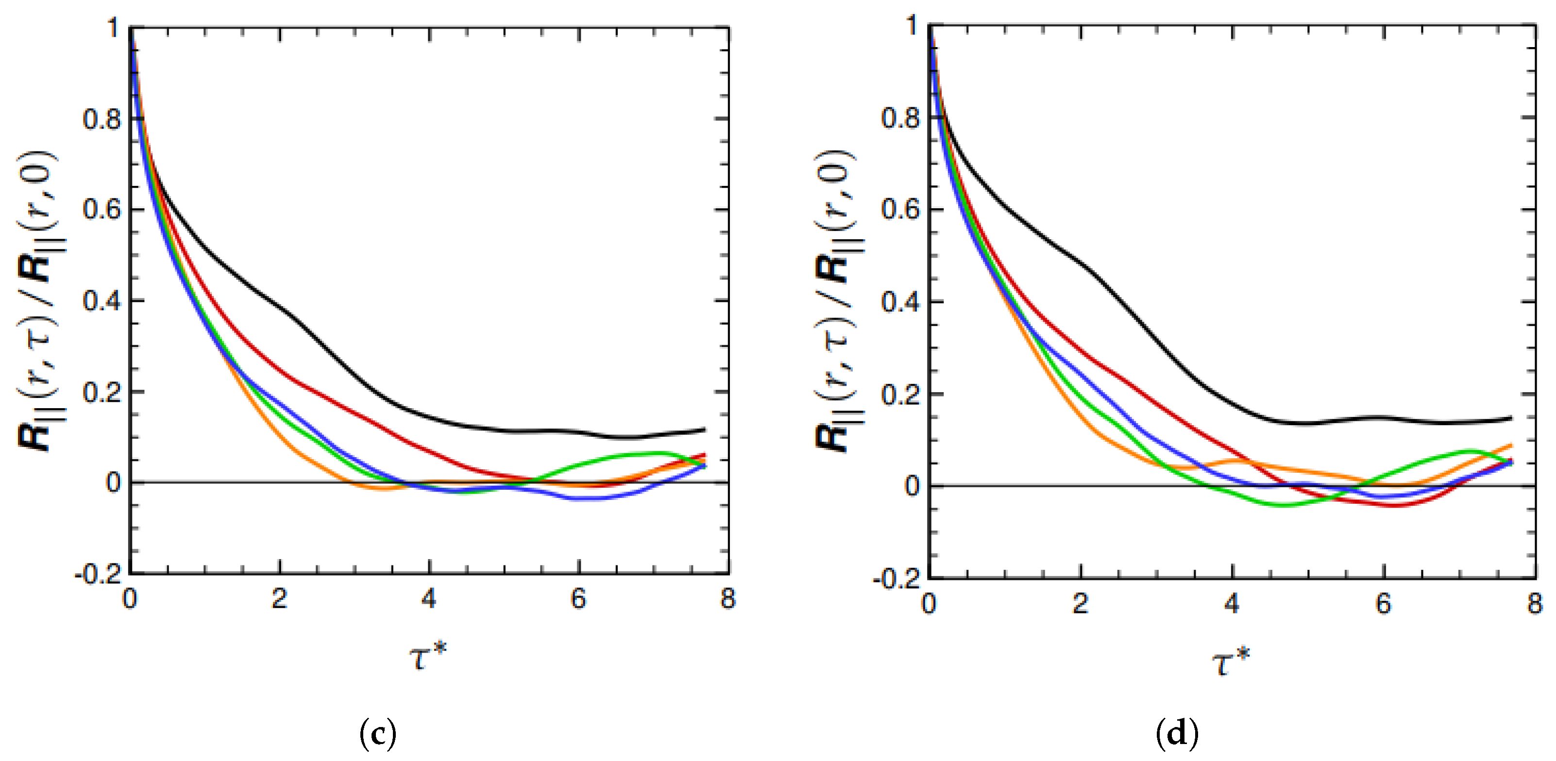
Figure 2. ${\mathit{R}}_{\perp }(r,\tau )={⟨\Delta \mathit{u}(\mathit{r},\mathit{x},0)\Delta \mathit{u}(\mathit{r},\mathit{x},\tau )⟩}_{\perp }$ as a function of dimensionless time separation, $\tau *=\tau u_{\mathrm{rms}}/L$, for $R{e}_{\lambda }=80$. (a) $r/L=0.56$, (b) $r/L=1.12$, (c) $r/L=2.24$, and (d) $r/L=3.36$.

As $R{e}_{\lambda }$ is increased, there is greater separation among the energy-containing and energy-dissipating scales. Hence, we expect to see a clearer illustration of the role of forcing scheme at higher $R{e}_{\lambda }$. The longitudinal correlations ${⟨\Delta \mathit{u}(\mathit{r},\mathit{x},0)\Delta \mathit{u}(\mathit{r},\mathit{x},\tau )⟩}_{\left|\right|}$ for $R{e}_{\lambda }=210$ are presented in Figure 3a–d at $r/L=0.56,1.12,2.24$, and $3.36$, respectively. It is amply evident that the DF longitudinal correlation is higher than the SF1–SF4 correlations (except at small $\tau *$). For separations $r>L$, we see that the DF correlation significantly exceeds the SF1–SF4 correlations. As shown in Figure 4, the transverse correlations exhibit the same behavior as well. From Equation (2), it can be seen that larger values of the longitudinal and transverse correlations result in enhanced diffusivity, ${\mathit{D}}_{UU}^{\left[1\right]}$, particularly at higher $R{e}_{\lambda }$.

Figure 3. ${\mathit{R}}_{\left|\right|}(r,\tau )={⟨\Delta \mathit{u}(\mathit{r},\mathit{x},0)\Delta \mathit{u}(\mathit{r},\mathit{x},\tau )⟩}_{\left|\right|}$ as a function of dimensionless time separation, $\tau *=\tau u_{\mathrm{rms}}/L$, for $R{e}_{\lambda }=210$. (a) $r/L=0.56$, (b) $r/L=1.12$, (c) $r/L=2.24$, and (d) $r/L=3.36$.

Figure 4. ${\mathit{R}}_{\perp }(r,\tau )={⟨\Delta \mathit{u}(\mathit{r},\mathit{x},0)\Delta \mathit{u}(\mathit{r},\mathit{x},\tau )⟩}_{\perp }$ as a function of dimensionless time separation, $\tau *=\tau u_{\mathrm{rms}}/L$, for $R{e}_{\lambda }=210$. (a) $r/L=0.56$, (b) $r/L=1.12$, (c) $r/L=2.24$, and (d) $r/L=3.36$.

4. Conclusions

This study was motivated by the observations in [2] regarding the behaviour of the three closure forms for the diffusivity tensor (CF1, CF2, and CF3) as the Reynolds number was increased. We were particularly interested in understanding why the CF1 diffusivity showed a significant increase with $R{e}_{\lambda }$ at separations $r\gtrsim L$. It was conjectured in [2] that this behaviour of CF1 was an artifact of the deterministic forcing scheme employed in the DNS run to compute the Eulerian two-time correlation of the relative fluid velocities that were an input to CF1.

To test this hypothesis, we performed a detailed investigation consisting of DNS runs with both deterministic and stochastic forcing schemes at $R{e}_{\lambda }\approx 80$ and $210$. For the stochastic forcing runs, we also considered the effects of varying the forcing time scale, $T_f$. A comparison of the Eulerian correlations from these simulations clearly establishes the fundamental premise of this study. This behaviour of DF may be anticipated since it involves, at every time step, the pumping of energy equal to the dissipated energy into the scales in a narrow band of low wavenumbers. As a result, the large scales are essentially kept from turning over for a longer duration than in a (DNS + SF) simulation, increasing their temporal coherence.