1. Introduction
Water erosion creates a severe type of soil erosion, as it is susceptible to make more impact on the soil surface compared to wind erosion. This is caused by rainfall, which is known as the major factor that contributes to water erosion because it causes the soil particle to become loose and detached. The mechanism of rainfall erosion i.e., topography, soil properties, and rainfall characteristics, has been investigated both by simulated and natural rainfall. The excess rainfall from saturated soil becomes surface runoff; this is known as a partial contributor to soil loss. Meanwhile, the energy of raindrops that detach the soil structure is another partial contributor. The factors affecting water erosion are divided into four main mechanisms, namely; characteristics of rainfall as well as surface runoff, properties of soil, and topography conditions.
Ref. [
1] stated that the three stages that describe the water erosion process are detachment, transport, and deposition of soil particles. Detachment is the first process to occur, which causes soil clods to break into smaller particles, and is considered an independent variable that plays an important role as no erosion can happen unless detachment takes place [
2]. Transportation is considered a dependent variable upon detachment. In shallow water conditions especially, raindrop splash provides temporary disturbances that caused static particles to move, which are then eventually transported by overland flow [
3,
4]. Deposition is considered a dependent variable upon the earlier two stages. A deposition may take place when sediment transport capacity is lesser than sediment load in the flow [
5].
Previous experimental and field works studied that soil erosion is influenced by hydraulic properties of flow, physical properties of soil, and surface characteristics [
6]. Rainfall intensity was determined as the main factor among the important parameters in predicting soil erosion [
7]. As an example, the authors of [
8,
9] found that high intensity rainfall produces maximum sediment load in the runoff. In a particular natural rainfall event, the intensity is rarely constant throughout the event, but it has a significant or a slight change in intensity. The total volume of runoff does not create a significant effect, regardless of intensity variation applied during the rainfall simulation, although it creates an impact on the sediment accumulated. The authors of [
10,
11,
12] found that soil loss is most governed by increasing rainfall patterns while the lowest loss is from the constant rainfall event. This is in contrast with a study by [
13] that found that the rising–falling rainfall produces the largest total runoff and soil erosion amount. They also found that at the same slope gradient, the relative difference between the total runoff and soil erosion amounts of different rainfall patterns was up to 111% and 381%, respectively.
Surface runoff, other than the result of raindrop impact, has been recognized as an erosive agent as it causes shear stress to the soil surface, which, if it exceeds the cohesive strength of the soil, would result in sediment detachment [
1]. Ref. [
14] studied the effects between three conditions of slope angle, rainfall intensity, and vegetation cover on the erosion characteristics, and found that sediment yield is significantly affected by rainfall intensity and least affected by slope angle. To study the effect of runoff flow rate on soil erosion, the present work of [
15] aims to simulate the dynamics of soil erosion, considering the three main parameters influencing the phenomenon; the nature of the soil (compaction), hillslope, and the rainfall intensity. The results showed that the larger flow rate gives a maximum mass of soil, which moves at about a five times increment compared to the smaller flow rate.
As cited by [
16], runoff erosion can individually cause soil degradation, disastrous floods, and droughts, as well as shortage of food supplies worldwide, but most erosion events are accompanied by the loss of nutrients that can cause unproductive farmlands and eutrophication on water bodies. The transported sediment may become siltation that can modify the river course and carry chemicals that can pollute the ecosystems [
17]. Therefore, erosion and sediment transport are related to each other as severe soil erosion led to a large amount of sediment discharged into water bodies. The erosion process and sediment transport can be represented by the model in three ways; empirical, conceptual, and physically based [
1]. The models differ greatly in terms of their complexity, their inputs and requirements, the processes they represent and the way in which these processes are represented, the scale of their intended use, and the types of output they provide. Empirical models are limited to conditions for which they have been developed [
6]; they are generally the simplest of all three model types [
1,
3], and usually use a smaller number of parameters [
16]. Empirical models also tend not to be event-responsive, ignoring the processes of rainfall-runoff in the modeled catchment. Nonetheless, empirical models are frequently used in preference to more complex models as they can be implemented in situations with limited data and parameter inputs; as [
1] stated, they are particularly useful as a first step in identifying sources of sediment generation. In conceptual models, a watershed is represented by storage systems [
1,
6] and tends to include a general description of catchment processes without including the specific details of process interactions, which would require detailed catchment information. Physically based models are based on the solution of fundamental physical equations describing stream flow and sediment generation in a catchment. Standard equations used in such models are the equation of conservation of mass and momentum of flow, and the equation of conservation of mass for sediment [
6]. More complex models are more likely to provide a better fit to calibration data, although this does not necessarily extend to providing better predictions of future behavior, as complex models run the risk of being over fitted by the calibration data.
Generally, previous studies aim to determine sediment transport by covering a wide range of hydraulic variables; total discharge [
18,
19,
20], bed shear stress [
12,
21], stream power [
20,
22,
23], and unit stream power [
12,
24]. Because rainfall intensity was investigated as the main factor in soil erosion, the objective of this study was to establish the selected parameters that contribute to the sediment transport capacity in overland flow under different rainfall pattern conditions and to evaluate their significance. This will contribute to the rainfall-runoff induced sediment transport mechanism, with the data from experimental work on an erosion plot filled with bare soil that had undergone four (4) different types of rainfall patterns. The selected parameters were used in developing empirical model equations for the calculation of sediment transport.
2. Methodology
The methodology used in this study to achieve the objectives will be explained further in this section based on subsections, namely; (i) experiment setup, (ii) determination of dimensionless dependent and independent parameters, and (iii) regression models and model performance.
2.1. Experiment Setup
The experimental data are derived from rainfall simulation using equipment, namely H313 Hydrology Apparatus from TecQuipment. The setup takes place at the Faculty of Civil Engineering, University Technology of MARA, Selangor, Malaysia. The runoff plot is 2.0 m (length) × 1.0 m (width) × 0.19 m (depth). The said plot provided a surface area of 2 m2 and a total volume of 0.38 m3. The system consists of eight pressurized spraying nozzles at the height of 0.8 m over the soil plot.
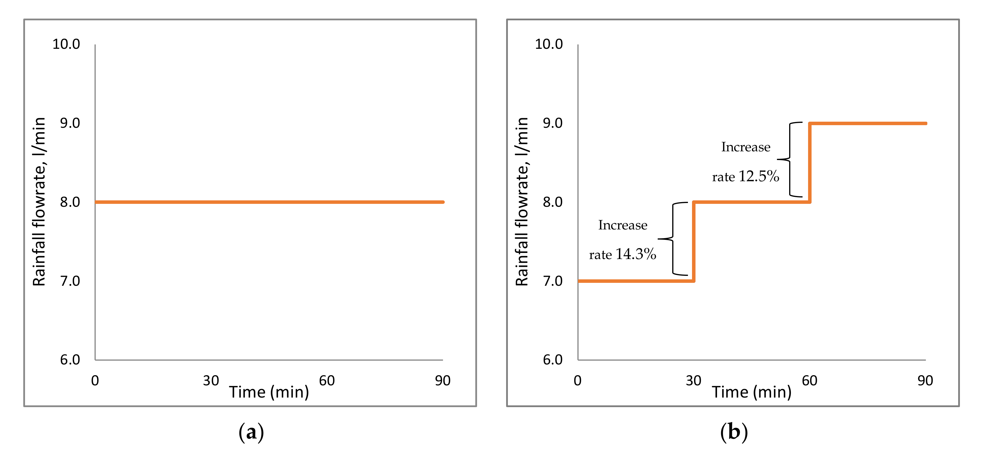
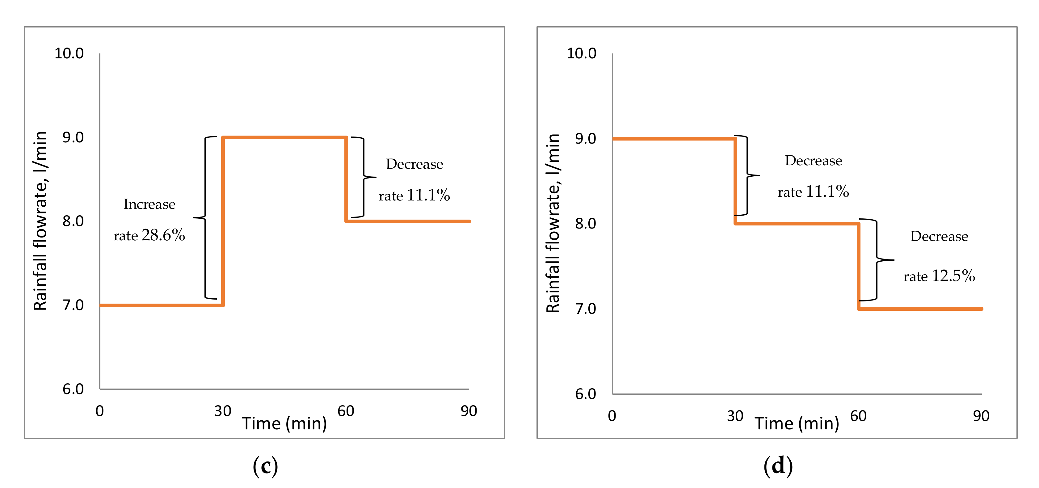
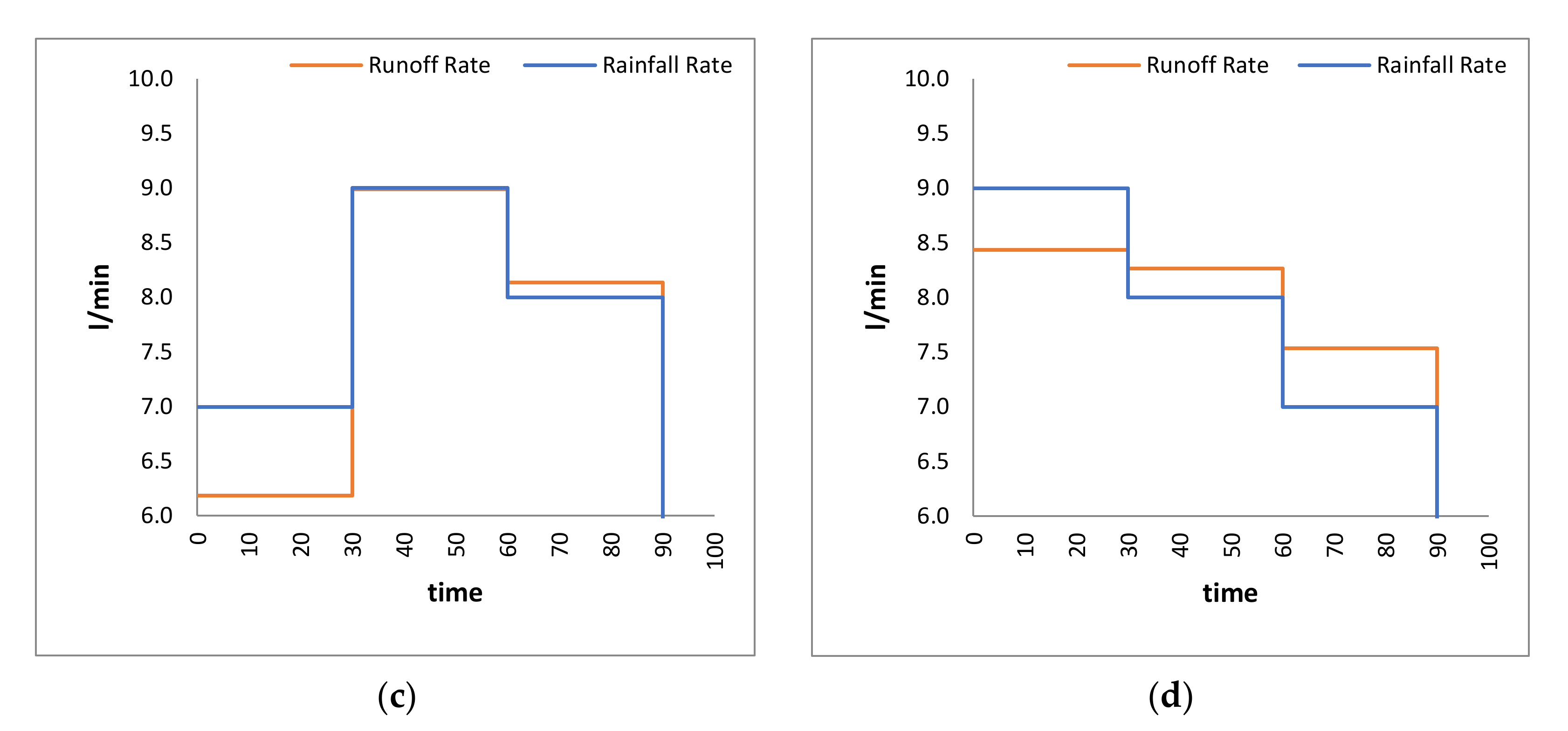
For this study, the applied water flow rate is varied from 7 to 9 L/min (equivalent to 210 to 270 mm/h). The average flow rate applied for every rainfall pattern was 8 L/min (240 mm/h), which means that rainfall intensity of about 30 mm/h was produced by each nozzle. The constant slope steepness of 7% was set throughout the experiment. A total of 12 datasets was derived from the experiment; 3 repetitions of 4 rainfall patterns, namely; constant-type (CST 8-8-8 L/min), increasing-type (ICR 7-8-9 L/min), increasing-decreasing-type (ICRDCR 7-9-8 L/min), and decreasing-type (DCR 9-8-7 L/min). Their respective increase and decrease rates that are set for the whole experiment are as shown in
Figure 1.
Each rainfall simulation has a total duration of 90 min. With the exception of the CST pattern,
Figure 1a, the changing of flow rate was performed every 30 min.
Table 1 shows the physical and chemical properties of the soil samples used, which are classified as sandy loam soil. From the soil particle size distribution curve, the median diameter of soil particle (
D50) of 0.36 mm was obtained. The compaction of soil in the plot was performed by filling layer by layer with the calculated soil volume to achieve the intended bulk density. To ensure the uniformity of soil height so that the flow depth can be fully covered the width direction, in the final soil layer compaction, a long stick is placed on the surface as the marker of straightness to the several marked heights at the inner side of the plot.
During simulation, about 500 mL volume of runoff samples was taken at 3-min intervals to ensure the best and presentable result data. The collection process was repeated until the runoff ended. In total, 30 samples were taken from each experiment. The runoff samples were left in the refrigerator at about 6 °C temperatures overnight to allow sediment to settle rapidly. On the next day, the samples with settled sediment were carefully removed from the refrigerator and the decanting process commenced to remove excess water. The decanted samples were then placed in the oven at 105 °C for 24 h. The dry sediment weight was then measured and recorded to obtain the sediment concentrations in the unit of mg/L or ppm. The procedure was repeated for every rainfall simulation.
2.2. Sediment Transport Prediction and Governing Equations
Ref. [
25] are among the earliest researchers that proposed the empirical models of sediment transport (
). The principal variables related to overland flow are as follows; length of slope (
L) and surface slope (
S) as the important geometric variables; rainfall intensity (
i), flow depth (
h), mean velocity (
), unit water discharge (
q), and thickness of laminar sublayer (
) are the hydraulic variables; bed shear stress (
) is the common parameter linked with sediment transport (
) as compared to gravitational acceleration (
g); and kinematic viscosity (
ν) and density of water (
ρ).
For overland flow conditions, slope and unit water discharge are assumed easier to be measured as compared to the velocity and depth of flow, thus the variables
S and
q are more favorable as the components of the sediment–transport relationship as compared to variables
ū and
h. The other variables used are
i and
L. This is different from the river flow conditions, where the variables
S,
ū,
h, and
q are used rather than
i and
L to express streamflow because they are easier to measure. On the other hand, critical shear stress (
) is correlated with the start of the sediment particle motion, where the fundamental relationship describes the initial motion of sediment. A study by [
26] shows that the relatively high value of critical shear stress (
> 0.15) contributes to stable bifurcation and indicates that no particle motion happens. The sediment size can be replaced by the
in the sediment equation as it is defined as the function of particle size and specific masses of water and sediment. The units and dimensions of the parameters used in the equation were summarized in
Table 2.
From the function of parameters mentioned earlier, a few relationships are used with the assumption of constant
ρ, the function is reduced to:
By considering repeating variables of
L,
ρ, and
v, the Π-terms function is gained from the dimensional analysis method. Then, experimental coefficients as
, β, γ, δ, and ε are introduced to obtain equation under dimensional form of:
The term
represented the sediment equations based on pulling force and stream power concepts. It is a factor that describes the soil resistance to erosion, and may reduce the remaining three factors,
S,
q, and
i that are corresponding to the potential erosion or transport capacity of overland flow. When
is very small compared to
, the above equation can be described as follows:
This is the version addressed by [
27], which begins on a straightforward equation for sediment transport capacity. It is commonly used in hillslope as well as in fluvial geomorphology. They recommended using values of 1.0 ≤ β ≤ 1.8 and 0.9 ≤ γ ≤ 1.8 in sediment transport modeling because there is no compelling evidence for one exponent to outweigh the other by a significant margin. The method used to characterize hydraulic resistance almost does not affect the exponents. The median value of each parameter β = γ = 1.4 may be selected if one is chosen to consider a single combination.
According to [
28], a function of the geometric, fluid flow, and soil variables is written as sediment transport from sheet erosion. This is the same from the version of the reduced function relationship described by [
25] (Equation (1)). Through dimensional analysis, the function is then transformed into three dimensionless parameters as follows:
The dimensional analysis resulted in a dimensionless sediment transport parameter to the function of the soil surface slope (S), the Reynolds number , dimensionless rainfall parameter , and the soil characteristics .
Ref. [
20] studied sediment transport capacity under the influence of unit discharge, mean flow velocity, and slope gradient. The experiments were conducted in a 3 m long by 0.5 m wide erodible bed using four well-sorted grains of sand and were simulated at four slope conditions. The equation is analyzed as promising to be applied in process-based soil erosion models, particularly in estimating sediment transport capacity. The proposed equation is as follows:
where
Q is the total discharge and
is the median grain diameter. The derived equations should be applied in a range of conditions of: unit discharge between 0.00007 and 0.00207 m
2s
−1;
S between 5.2 and 17.6%; and
between 0.233 and 1.022 mm.
Ref. [
16] made a simple relationship analysis of affecting variables; the dependent variable,
, and the independent variables:
S,
q,
i, and
. The
is introduced as an independent variable from the earlier equations by [
28]. The several combinations of independent variables are chosen and applied as four different models, namely Model 1 to Model 4. F-tests and t-tests method are used to test the impact of the models and parameters by calculating the F and t statistics for each model, respectively. The calculated value that is larger than the equivalent critical value is defined as significant.
The four models used in this regression-based empirical model are as follows:
The Genetic Algorithm (GA) optimization method is applied in order to obtain the ideal values for all coefficients and exponents in the four proposed regression models. A total of 80 instances of rainfall-runoff influenced by sediment transport are conducted for this study. All the experiments are performed on erosion flumes. From the data, 64 samples of data are chosen randomly as the calibration process and the balance is used in the validation stage. The data of the simulated sediment transport rates versus the experimental observations in the calibration stage and validation stage are plotted and form the graph; it is concluded that Model 4 with parameter included shows the best data evaluation compared to the other three.
2.3. Determination of Dimensionless Dependent and Independent Parameters
From the previous governing equations in
Section 2.2, the factors affecting sediment transport can be categorized into three; hydraulic characteristics, sediment characteristics, and hydraulic geometries. These categorizations are adapted from the study by [
29]. All empirical relations have used dimensionless parameters, which have been proved meaningful and applicable to various systems of units.
Table 3 shows the significant independent parameters by the various researchers with respect to dependent variable sediment transport (
).
2.3.1. Parameter Class and Selected Variables
As previously discussed, the primary factors that affect water erosion in expressions of sediment transport are divided into three categories, namely hydraulic characteristics, sediment characteristics, and hydraulics geometries. The most physical variable can be written in terms of three basic dimensions (M, L, and T) and are classified as geometric, kinematic, or dynamic, or classified as dimensionless variables where no SI unit is defined [
28].
The selected variables with their units and dimensions are presented in
Table 4. The listed variables were tested on their significance with the dependent variable sediment transport,
by a dimensional analysis approach, which will be explained further.
Fluid density, is referred to as the mass of fluid per unit volume. The maximum density of water 1000 kg/m3 is at approximately 5 °C and slightly decreases with temperature. The same condition is also observed in the kinematic viscosity, ν as it is derived from dynamic viscosity, μ divided by density, that causes mass terms to cancel out.
2.3.2. Dimensional Analysis
Describing the independent variables to the dependent variables and testing the consistency of the dimensions of all variables can be achieved by dimensional analysis. Dimensional analysis should meet these objectives; (1) reducing the numbers of variables before analysis of the problem is performed and (2) providing dimensionless parameters, in which the numerical values are not dependent on any system of units. From the set of variables as shown in
Table 4, the functional relationship between water erosion in terms of sediment transport with the governing factors was determined [
28].
In this study, the dimensional analysis was conducted using Buckingham’s Π theorem. Buckingham’s Π theorem allows for rearranging n-variables where there are j fundamental dimensions to obtain the n−j dimensionless parameters. The theorem allows the dependent variable
to be connected to a functional relationship
f of independent variables, as listed in
Table 4, such that:
For dimensional analysis purposes, the above equation can then be reduced and expressed in the relationship of:
Applying theory from [
25], parameter
can be omitted by assuming
was very small compared to
,
S is maintained as independent dimensionless variables, and for the remaining variables, n is 8. With j fundamental dimensions involved when parameters are converted into three basic units of the system; mass M, length L, and time T, makes j = 3 and the relation is lessened to a function of n−j = 8−3 = 5 dimensionless π parameters. The above relationship is then expressed as Π
1 until Π
8 form as:
Thus, to represent j fundamental dimensions, three repeated independent variables were chosen, which are;
L,
ν, and
. Dimensions for each selected variable are shown in the equation below:
Then the five π parameters are gained from replacing the fundamental dimensions in the above functional relationships for
,
q,
i,
Q, and
, respectively:
The dimensionless parameters that express a functional relationship between dimensionless sediment transport and the independent parameters can thus be written as:
From theory, the parameter
can be replaced with Reynolds number (
Re) defined as the ratio of the relative magnitude of inertia and viscous forces in which the condition of inertia forces mostly overcomes the viscous forces. Large
Re shows that the flow is turbulent, for example in rivers and gullies. In the opposite situation, named laminar flows happen on thin overland runoff [
25]. Reduced flow depth may limit the transport of sediment by saltation and suspension in overland flow for certain particle sizes.
Re can be simplified as:
where:
= fluid density (kg/m3)
V = flow velocity (m/s)
L = length of flow (m)
μ = dynamic viscosity of fluid (kg/ms)
ν = kinematic viscosity of fluid (m2/s)
Hence, the dimensional analysis results form a dimensionless sediment transport parameter function of the Reynolds number, a dimensionless rainfall parameter, hydraulic characteristics, soil characteristics, and surface slope. The parameter classes and respective dimensionless groups are shown in
Table 5.
From the dimensionless parameters listed in
Table 5, parameter
S,
, and
however are the constant values obtained from the experimental data and could be eliminated. Therefore, with consideration of
Re and these constant values, the final relationship shown in Equation (16) can be written as:
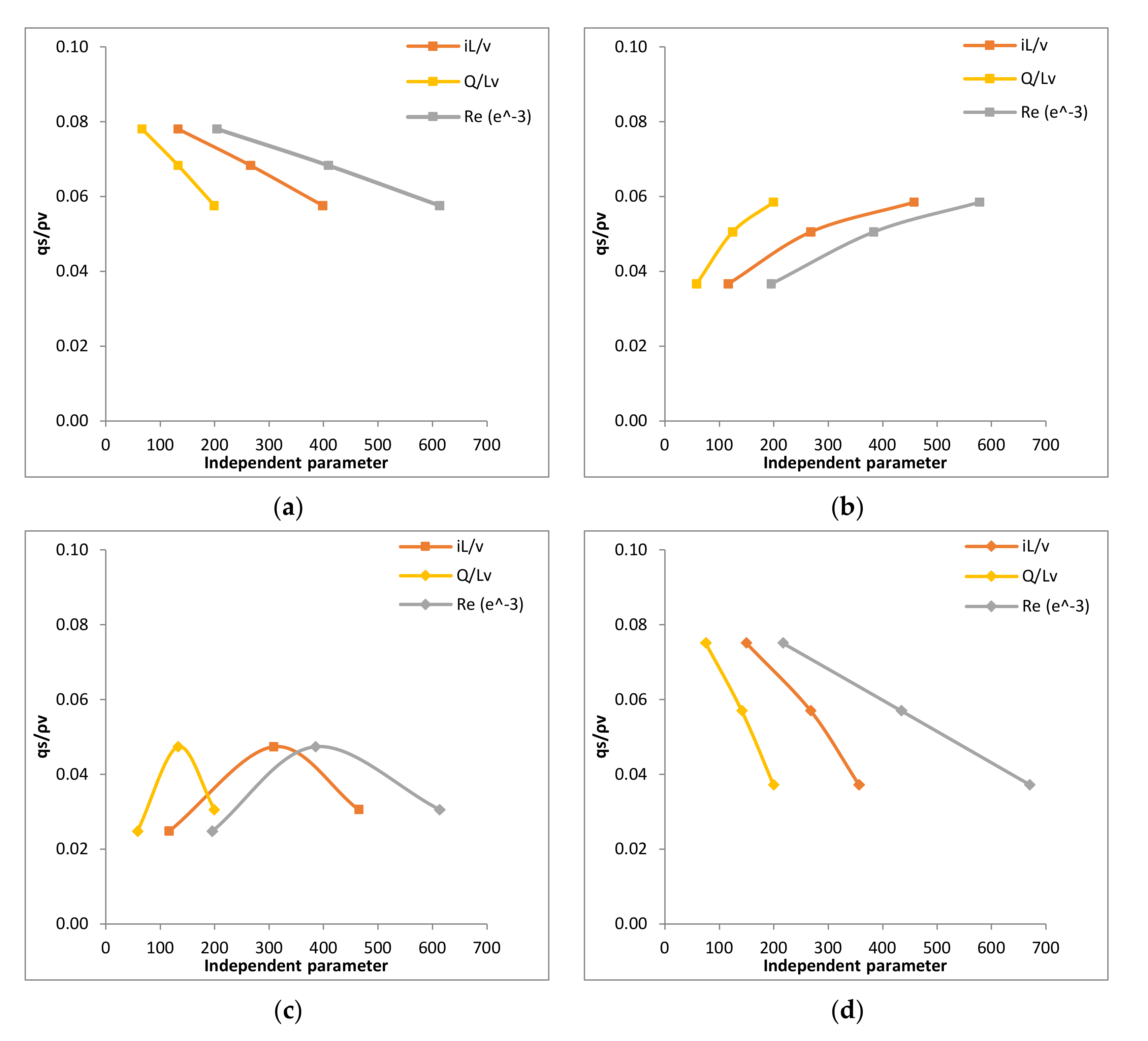
The relationship of these independent parameters
against dependent parameters
has been plotted as in
Figure 2 and
Figure 3.
2.4. Regression Models and Model Performance
Statistical approach from the 12 experiments was used to predict models for quantifying sediment transport. Regression methods used are linear and nonlinear models. Linear models use basic regression theoretical derivation formula while nonlinear models use basic power relationship between the dependent and independent parameters. Model performance was checked by the prediction accuracy (R2) value from the regression analysis.
Model validation uses discrepancy ratio (DR) method, which is the ratio of the predicted to the measured values. Predicted values are derived from the model equations with high value of R2. The model equation is assumed to have good prediction when the predicted values have similar values with the measured values. The values are considered to be correctly satisfactory if the data lie within 0.5–2.0 limit of the line of perfect agreement.
3. Relationship of Dependent Parameters against Independent Parameters
From the functional relationship developed in Equation (18), the graph was plotted to describe the relationship and the significance of against each independent parameter.
The sediment concentration data (in mg/l) were then converted to unit kilogram to find the value of the measured dependent parameter
.
Re was calculated using a formula of
, however, velocity was found first by dividing
Q with the cross-sectional area of flow; wherein this study used a constant value of flow width,
B of 1m. The physical properties of water used were based on the normal temperature of tap water of 20 °C. Using the value of known flow rate of 1.167 × 10
−4, 1.333 × 10
−4 and 1.50 × 10
−4 m
3/s for each rainfall intensity applied produced 210, 240, and 270 mm/h, respectively, and constant slope steepness of 0.07, the flow depth, and
h were calculated from area of flow, and the wetted perimeter for rectangular channel was embedded in the Manning’s equation:
where:
From the plotted graph in
Figure 2, the relationships for all three parameters are showing the same increasing trend, with the scatter pattern slightly different between each other. However, when plotted based on different rainfall patterns as in
Figure 3, it shows the scatter trend showing the same pattern with the increasing and decreasing intensities during rainfall simulation; nevertheless, for the CST type, the trend shows a decreasing trend. The value was synchronized with the actual duration and the time of each rainfall simulation. This was performed by multiplying the measured value with the time of changing flow rate throughout the simulation, as mentioned earlier; 30 min in total duration of 90 min rainfall simulation.
Figure 2a,b show the plotted graph of the dependent parameter against
and
, respectively. Both graphs show the increasing trend. The four variables involved in this parameter are rainfall intensity (
i), length of runoff (
L), kinematic viscosity (
ν), and total discharge (
Q). From these four variables, two of them,
L and
ν, may be constant for all simulations, while the other two,
i and
Q, are changed in this study. In this study, the increasing of
i (ranging from 0.21 to 0.27 m/s) produced increasing
Q (ranging from 1.167 × 10
−4 to 1.5 × 10
−4 m
3/s) that increased the transportations of the sediment in the flow.
Figure 2c shows the dependent parameter against
Re parameter. The calculated
Re obtained in this study varied between 190,000 and 670,000, indicating the flow in highly turbulent conditions.
Re is defined as the ratio of the relative magnitude of inertia and viscous forces, in which the condition of inertia forces mostly overcomes the viscous forces. From the experimental data, the calculated flow depth for the respective flow rate ranges from 1.19 mm to 1.38 mm.
Table 6 presented the best fitting equation that was selected for the determination of the coefficients of the best-fitted trend line. Meanwhile,
Table 7 shows the same analysis but with the consideration of different rainfall pattern conditions. The relationship between dependent and independent parameters can all be described in the power functions (R
2 > 0.636). The fitting equation and coefficients for the combination of all data without considering the rainfall patterns are also included in the table. The R
2 value of 0.636 for the relationship of
with
, 0.724 with
, and 0.692 for relationship with
Re. This indicates that 63.6% and 72.44% of the variance in the independent parameters is to the dependent parameter
without considering rainfall pattern conditions.
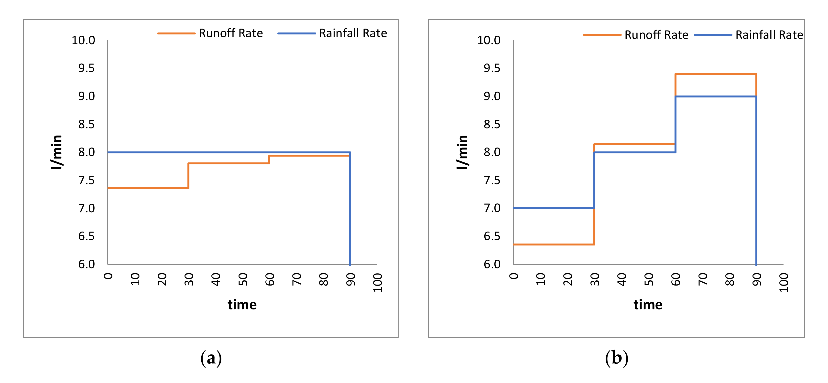
Figure 4 shows the comparison of rainfall and runoff rate for each rainfall pattern. Runoff produced starts to increase significantly and then stabilizes during the first 30-min duration of rainfall. After stabilizing, the runoff seems to show the same pattern as the intensity in the following duration through the end. This is due to the rainfall volume at the beginning of the duration filling the infiltration capacity in the soil plot until it produces runoff.
The summary relationship of increasing and decreasing rate of rainfall pattern on runoff rate and the range of dependent parameter,
is shown in
Table 8. The range of
is derived from the plotted graph in
Figure 3 for their respective rainfall patterns. From these graphs, the clear observation in the range of
; 0.058 to 0.078 for CST, 0.036 to 0.058 for ICR, 0.025 to 0.047 for ICRDCR, and 0.037 to 0.075 for DCR rainfall pattern. For CST-type, although the rainfall rate was set to be constant for the 90-min duration, the runoff rate shows that there is increasing value, but further analysis shows that it does not have significant impact in the value of
.
The analysis concludes that the sediment transportation happened severely in DCR, meanwhile the least happened in the ICRDCR rainfall pattern. The findings are in contrast with the studies of [
7,
12,
30], which found an increasing pattern that contributed the highest amount of soil loss. However, it is consistent with [
10], which found that a decreasing pattern produces the highest loss, which is similar to this study’s findings. The difference in these findings is due to the intensity of rainfall used being different for each study; soil loss may happen severely in an increasing pattern where the rainfall intensity measured is below 100 mm/h but for intensity more than that, such as the intensity used in [
10] (100–160 mm/h) and this study (210–270 mm/h), the severe soil loss happened in a decreasing pattern. This is because the higher intensity applied in the first phase of rainfall duration results in a higher capacity of raindrop hits on soil plots, which causes splash erosion. Other than that, the contrast in findings may have happened due to the total duration of rainfall. The loose particles were carried out with the surface runoff, shown by the figure where the early phase has the highest concentrations until it reaches a stable mode through the end of the rainfall duration.
Table 9 shows the results from the SPSS curve estimation analysis to better define the relationship between the dependent parameter and each assigned independent parameter. From the analysis, multiple nonlinear regression has a high obtained R
2 value compared to the multiple linear regression. However, from both regression methods, the F and P values show that the independent parameters are statistically significant to the dependent parameter (
p < 0.05).
To find the relationship of all three independent parameters to the dependent parameter, the iteration method was used in the SPSS software. Iteration method is the estimation of coefficients by repeated approximations process with a set starting value. It continues until the estimated coefficients converge or reach the maximum number of attempts. From the iteration results in
Table 10, the estimation of constant and regression coefficient values is given. This value can be presented in the form of the general formula for linear and nonlinear model equations. The highest R
2 value of 0.931 is derived from multiple linear regression with all independent parameters included in the developed equation (Equation (23)). The same significant factor can be evidenced in Equation (27) with model accuracy of 0.815.
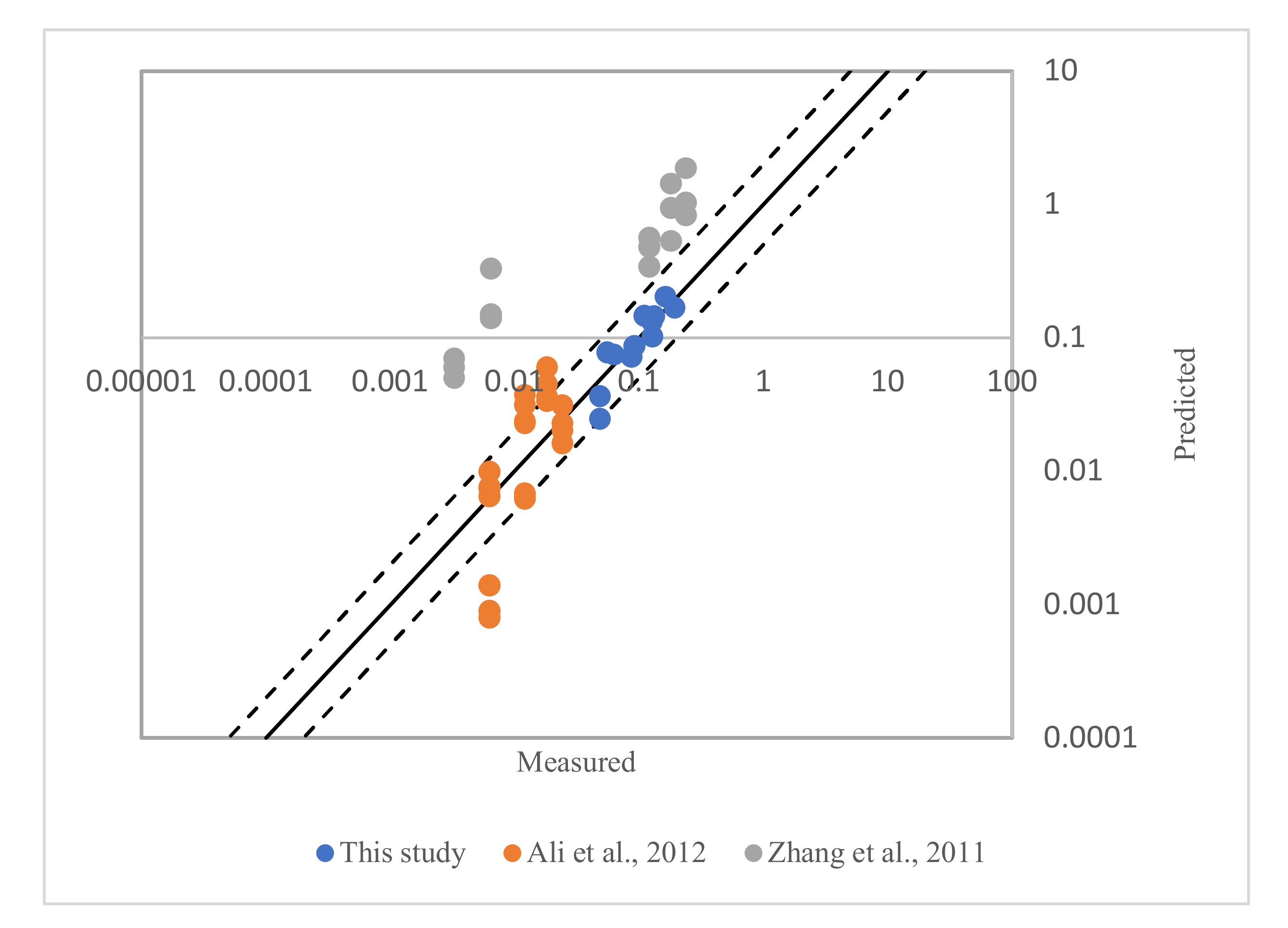
Figure 5 shows the agreement between measured and predicted dependent parameters,
using the dataset from this study. The graph plotted is validated using Discrepancy Ratio (DR) method. The model equation is considered accurate when the data of measured and predicted values lie between 0.5 and 2.0 limits (shown by the dashed line). From the two equations with the highest model accuracy value (Equations (23) and (27)), both are tested under DR. The data from the experiments were used along with the data from [
20,
31]. The highest percentage of DR derived was 54.9% using Equation (27).
