Calibration of Thixotropic and Viscoelastic Shear-Thinning Fluids Using Pipe Rheometer Measurements

Abstract

Some non-Newtonian fluids have time-dependent rheological properties like a shear stress that depends on the shear history or a stress overshoot that is a function of the resting time, when fluid movement is started. The rheological properties of such complex fluids may not stay constant while they are used in an industrial process, and it is therefore desirable to measure these properties frequently and with a simple and robust device like a pipe rheometer. This paper investigated how the time-dependent rheological properties of a thixotropic and viscoelastic shear-thinning fluid can be extracted from differential pressure measurements obtained at different flowrates along a circular pipe section. The method consists in modeling the flow of a thixotropic version of a Quemada fluid and solving the inverse problem in order to find the model parameters using the measurements made in steady-state conditions. Also, a Maxwell linear viscoelastic model was used to reproduce the stress overshoot observed when starting circulation after a resting period. The pipe rheometer was designed to have the proper features necessary to exhibit the thixotropic and viscoelastic effects that were needed to calibrate the rheological model parameters. The accuracy of rheological measurements depends on understanding the effects that can influence the observations and on a proper design that takes advantage of these side effects instead of attempting to eliminate them.

1. Introduction

Many industrial processes make use of non-Newtonian fluids. It is common that these non-constant viscosity fluids are also thixotropic and viscoelastic. This is the case for paints [1], drilling fluids used in well construction [2], some products used when making food or cosmetics [3] and even fluids in the medical domain, such as blood [4].

Using computer-controlled rheometers, it is possible to obtain flow curves to relate the shear stress to the shear rate and therefore characterize the steady-state rheological behavior of fluids [5]. It is also possible to measure the hysteresis obtained when performing a sweep from high to low shear rates followed by another one from low to high shear rates, in order to quantify the thixotropic response of fluids [6]. It is also possible to perform oscillatory measurements to acquire information about the storage and loss moduli of viscoelastic fluids [7].

However, the fluid rheological properties may change sufficiently fast during an industrial process such that it is not practical to only rely on sporadic laboratory measurements, and a more continuous method for acquiring the fluid rheological properties is desirable. Some attempts have been made using the Couette concentric cylindrical geometry as an automated rheometer with automatic feed of fluid samples and associated automatic cleaning processes [8]. But the use of oil or other non-miscible liquids in the composition of the fluid can make the cleaning process very difficult when using water-based standard cleaning fluids, leading to a rapid deterioration of the measurement accuracy.

An alternative solution consists in using a pipe rheometer [9]. In a pipe viscosimeter, the pressure drop along a tube is measured at different flowrates, and the rheological behavior of the fluid is inferred from those measurements (see Figure 1). It is composed of a pump, a flowmeter, a measurement pipe section with a constant diameter and a differential pressure sensor across the measurement pipe section. The inlet of the pump is connected to a tank which contains the fluid that shall be measured. Typically, the tank has an internal circulation mechanism to avoid settling or gelling. The ports of the differential pressure sensor are sufficiently far away from the entrance and exit of the pipe section to ensure that the flow is fully developed at the measurement points. Here, the internal pipe radius is denoted by $R$. The pressure differential, $\Delta p$, is often measured over a long distance, $\Delta d$, to increase the sensitivity of the measurement.

This design is suitable for non-thixotropic fluids. However, if the fluid shear stress depends on the shear history, the measured pressure gradient can still be influenced by the passage of the fluid into the pump and possible other sources of shear rate variations encountered along the hydraulic circuit such as changes in the diameters or bends. Also, complex fluids may be viscoelastic. The simple design in Figure 1 is not well adapted to measure viscoelastic properties, and often the pipe viscometer is supplemented with a Couette rheometer to extract information about the viscoelastic behavior of the fluid. This is a source of problems when cleaning the concentric cylindrical rheometer, as mentioned above.

The question addressed in this paper was, therefore, how a pipe rheometer should look like to measure the viscous properties of a thixotropic fluid and how the viscoelastic parameters of the fluid can be calibrated.

The paper describes, in a stepwise manner, how to arrive at the proposed design of a thixo-elastic pipe rheometer. In the Section 2, the known equations and knowledge that will be used afterward to design the pipe rheometer are presented. In particular, it is proposed to use the Quemada rheological behavior [10] to describe the fluid, as there is a natural way to introduce thixotropy in that model. Section 3 explains how to calibrate a non-thixotropic Quemada model using a pipe rheometer. In Section 4, thixotropy is addressed. The original design of the pipe rheometer is modified to allow measuring one specific parameter of the thixotropic Quemada model in addition to the steady-state Quemada model parameters. Section 5 incorporates viscoelastic modelling and calibration. The design of the pipe rheometer is again modified to allow measuring the remaining thixotropic parameters of the Quemada model as well as the viscoelastic properties of a Maxwell linear viscoelastic model. A discussion about the advantages and weaknesses of the proposed pipe rheometer design is presented in Section 6. The conclusions are summarized in Section 7.

2. Background

Using the Navier–Stokes equation in steady-state conditions, it can be demonstrated that the shear stress at the wall in a circular pipe is directly proportional to the pressure gradient, regardless of the rheological behavior of the fluid [11]:

$${\tau }_w=\frac{R}{2}\frac{dp}{ds},$$

(1)

where $R$ is the internal pipe radius, ${\tau }_w$ is the shear stress at the wall, $s$ is the curvilinear abscissa along the pipe, and $\frac{dp}{ds}$ is the pressure gradient along the pipe.

One early reference to a pipe rheometer [12] utilized the Rabinowitsch–Mooney relation to determine the shear rate at the wall of the pipe based on the pressure gradient:

$${\dot{\gamma }}_w=\frac{3}{4}{\dot{\gamma }}_{N,w}+\frac{1}{4}{\dot{\gamma }}_{N,w}\frac{d\ln \left({\dot{\gamma }}_{N,w}\right)}{d\ln \left({\tau }_w\right)},$$

(2)

where ${\dot{\gamma }}_{N,w}=\frac{4Q}{\pi R^3}$ is the shear rate at the wall for a Newtonian fluid, and $Q$ is the volumetric flowrate.

An expression for $\frac{d\ln \left({\dot{\gamma }}_{N,w}\right)}{d\ln \left({\tau }_w\right)}$ was found for the Herschel–Bulkley rheological behavior [13], when $\tau ={\tau }_{\gamma }+K{\dot{\gamma }}^{n_{HB}}$, where ${\tau }_{\gamma }$ is the yield stress, $K$ is a consistency index, and $n_{HB}$ is a flow behavior index. The expression is:

$$\frac{d\ln \left({\dot{\gamma }}_{N,w}\right)}{d\ln \left({\tau }_w\right)}=\frac{d\ln \left(Q\right)}{d\ln \left({\tau }_w\right)}=\frac{n_{HB}+1}{n_{HB}}\frac{{\tau }_w}{{\tau }_w-{\tau }_{\gamma }}-\frac{C_1{\tau }_w+2C_0}{C_2{\tau }_w^2+C_1{\tau }_w+C_0}-1,$$

(3)

where $C_0=\left(6n_{HB}-4n_{HB}^2\right){\tau }_{\gamma }^2$, $C_1=2n_{HB}{\tau }_{\gamma }\left(1+n_{HB}\right)$, and $C_2=\left(1+n_{HB}\right)\left(1+2n_{HB}\right)$.

A pipe rheometer can use a straight pipe or a helical one, as described in [14]. However, the flow of a fluid in a helical pipe is subject to centrifugal forces that may separate some of the components of the fluid when they have different mass densities. As a result, the measured pressure drop may not be necessarily representative of the fluid mix. Therefore, from now on, only a configuration using a straight pipe will be considered.

Considering that the shear rate at the wall can be found from the volumetric flowrate and the shear stress at the wall, and that the shear stress at the wall is directly related to the pressure gradient, it is possible to obtain a flow curve of the fluid, i.e., $\tau =f\left(\dot{\gamma }\right)$, at as many discrete values as there are volumetric flowrate measurements, $\left\{\left(Q_1,\frac{d{p}_1}{ds}\right),\dots ,\left(Q_n,\frac{d{p}_m}{ds}\right)\right\}\to \left\{\left({\dot{\gamma }}_1,{\tau }_1\right),\dots ,\left({\dot{\gamma }}_m,{\tau }_m\right) \right\}$, where $m$ is the number of individual steady-state volumetric flowrates.

Depending on the chosen rheological behavior, the flow curve points can be used to fit the rheological model parameters. Typically, this is done by solving a minimization problem of the form [15]:

$$\left(a_1,\dots ,a_k\right)=\underset{\left(a_1,\dots ,a_k\right)}{\arg \min }{\sum }_{i=1}^m{\left({\tau }_i-\widehat{\tau }\left({\dot{\gamma }}_i\right)\right)}^2,$$

(4)

where $\widehat{\tau }$ is the rheological model, and $\left(a_1,\dots ,a_k\right)$ are the model parameters.

There are several possible candidates for the rheological model, but amongst them, the model proposed by Quemada [10] is particularly interesting. This is, first, because it is derived from physical principles, and second, because it provides a very good fit to many different shear-thinning fluids such as drilling muds [15] or biological fluids like blood [16]. The Quemada rheological behavior is:

$$\tau =\dot{\gamma }{\eta }_{\infty }{\left(\frac{{\dot{\gamma }}_c^{n_Q}+{\dot{\gamma }}^{n_Q}}{\chi {\dot{\gamma }}_c^{n_Q}+{\dot{\gamma }}^{n_Q}}\right)}^2,$$

(5)

where ${\eta }_{\infty }$ is the viscosity when $\dot{\gamma }$ tends to $\infty$, ${\dot{\gamma }}_c$ is a reference shear rate, $n_Q$ is a flow behavior index, and $\chi =\sqrt{\frac{{\eta }_{\infty }}{{\eta }_0}}$, with ${\eta }_0$ being the viscosity when $\dot{\gamma }$ tends to $0$. A third reason why the Quemada model is interesting is that it is built using thixotropic assumptions. For shear-thinning fluids, it is very common that ${\eta }_0$ is a very large number and, therefore, that ${\eta }_0\gg {\eta }_{\infty }$, meaning that $\chi \approx 0$. In that case, Equation (5) is reduced to:

$$\tau =\dot{\gamma }{\eta }_{\infty }{\left(\frac{{\dot{\gamma }}_c^{n_Q}+{\dot{\gamma }}^{n_Q}}{{\dot{\gamma }}^{n_Q}}\right)}^2,$$

(6)

In this paper, only shear-thinning fluids were considered, and it was assumed that $\chi =0$. In that condition, it was possible to derive a time-dependent version of the Quemada model [17]:

$$\eta ={\eta }_F{\left(\left(1-\left(1+{\kappa \lambda }_{t=0}\right)\mathsf{\Phi }\right)e^{-K_1\left({\left(\frac{\dot{\gamma }}{{\dot{\gamma }}_c}\right)}^{n_Q}+1\right)t}\pm \sqrt{\frac{{\eta }_F}{{\eta }_{\infty }}}\frac{{\dot{\gamma }}^{n_Q}}{{\dot{\gamma }}_c^{n_Q}+{\dot{\gamma }}^{n_Q}}\left(e^{-K_1\left({\left(\frac{\dot{\gamma }}{{\dot{\gamma }}_c}\right)}^{n_Q}+1\right)t}-1\right)\right)}^{-2},$$

(7)

where $\eta$ is the effective viscosity, $t$ is time, ${\eta }_F$ is the Newtonian viscosity of the background fluid, $\kappa$ is the compactness factor, $K_1$ is a shear rate entering in the differential equation governing the structure parameter, and $\mathsf{\Phi }$ is the normalized particle concentration. In addition, ${\lambda }_{t=0}$ is the value of the structure parameter in the initial conditions.

In [17], it was also established that the structure parameter in a completely unstructured state, denoted by ${\lambda }_{\infty }$, is defined as:

$${\lambda }_{\infty }=\frac{1}{\kappa }\left(\frac{1}{\mathsf{\Phi }}\left(1\pm \sqrt{\frac{{\eta }_F}{{\eta }_{\infty }}}\right)-1\right),$$

(8)

Similarly, the structure parameter in a fully organized state, i.e., when the shear rate tends to zero, has a value denoted by ${\lambda }_0$ that is expressed as follows:

$${\lambda }_0=\frac{1}{\kappa }\left(\frac{1}{\mathsf{\Phi }}\left(1\pm \sqrt{\frac{{\eta }_F}{{\eta }_0}}\right)-1\right),$$

(9)

Also, Quemada explained how viscoelasticity can be modelled using a thixo-elastic Maxwell model [18]:

$$\tau +\frac{\eta }{E}\dot{\tau }=\eta \dot{\gamma },$$

(10)

where $E$ is an elastic modulus that depends on time. It should be noted that in Equation (10), $\eta$ is a function of both $\dot{\gamma }$ and time due to thixotropic effects. A similar approach based on the Kelvin–Voigt viscoelastic model was recently described [19]. The solution of Equation (10) is:

$$\tau \left(t\right)=\tau \left(0\right)e^{-F\left(t,0\right)}+{\int }_0^{t}E\left(t^{\prime }\right)e^{-F\left(t,t^{\prime }\right)}\dot{\gamma }\left(t^{\prime }\right)d{t}^{\prime },$$

(11)

where

$$F\left(t,t^{\prime }\right)={\int }_{t^{\prime }}^t\frac{E\left(t^{″}\right)}{\eta \left(t^{″}\right)}d{t}^{″},$$

(12)

Considering the start of the fluid movement at time $t=0$, Quemada further argued that the elastic modulus is roughly proportion to the structure parameter:

$$E=E_0\lambda \left(t\right),$$

(13)

where $E_0$ is a constant after the fluid movement has started.

Note that the structure parameter is expressed as [17]:

$$\lambda \left(t\right)=\frac{\left({\lambda }_{\infty }{\left(\frac{\dot{\gamma }}{{\dot{\gamma }}_c}\right)}^n+{\lambda }_0\right)}{{\left(\frac{\dot{\gamma }}{{\dot{\gamma }}_c}\right)}^n+1}+\left({\lambda }_0-\frac{\left({\lambda }_{\infty }{\left(\frac{\dot{\gamma }}{{\dot{\gamma }}_c}\right)}^n+{\lambda }_0\right)}{{\left(\frac{\dot{\gamma }}{{\dot{\gamma }}_c}\right)}^n+1}\right)e^{-K_1\left({\left(\frac{\dot{\gamma }}{{\dot{\gamma }}_c}\right)}^n+1\right)t},$$

(14)

Furthermore, it was established that the stress overshoot after gelling is a logarithmic function of the gel time [20]. Gjerstad formulated this result as follows [19]:

$${\tau }_{os}\left(t_{gel}\right)={\tau }_{os}\left(t_{{gel}_1}\right)+\left({\tau }_{os}\left(t_{{gel}_2}\right)-{\tau }_{os}\left(t_{{gel}_1}\right)\right)\frac{\ln t_{gel}-\ln t_{{gel}_1}}{\ln t_{{gel}_2}-\ln t_{{gel}_1}}, \forall t_{gel}\ge t_{{gel}_0},$$

(15)

where $t_{gel}$ is the gel duration, ${\tau }_{os}$ is the stress overshoot, $t_{{gel}_1}$ and $t_{{gel}_2}$ are two gel durations for which the stress overshoot was measured, and $t_{{gel}_0}$ is a minimum gel duration for which this relationship is valid, typically one or two seconds.

Moreover, the pressure drop in steady-state conditions along a circular pipe was derived for a Quemada fluid using the Weissenberg–Rabinowitsch–Mooney–Schofield relation of the flowrate as a function of the shear rate and shear stress in a cross section [21]:

$$Q=\frac{\pi R^3}{{\tau }_w^3}{\int }_0^{{\tau }_w}\dot{\gamma }{\tau }^{2}d\tau =\frac{\pi d_w^3}{8{\tau }_w^3}{\mu }_{\infty }^3\left(\sum _{i=0}^6\frac{{\alpha }_i{\dot{\gamma }}_w^{4-i{n}_Q}}{4-i{n}_Q}\right),$$

(16)

where ${\alpha }_0=1$, ${\alpha }_1=2{\dot{\gamma }}_c^{n_Q}\left(3-n_Q\right)$, ${\alpha }_2=5{\dot{\gamma }}_c^{2n_Q}\left(3-2n_Q\right)$, ${\alpha }_3=20{\dot{\gamma }}_c^{3n_Q}\left(1-n_Q\right)$, ${\alpha }_4=5{\dot{\gamma }}_c^{4n_Q}\left(3-4n_Q\right)$, ${\alpha }_5=2{\dot{\gamma }}_c^{5n_Q}\left(3-5n_Q\right)$, ${\alpha }_6={\dot{\gamma }}_c^{6n_Q}\left(1-2n_Q\right)$.

In unsteady flow conditions, it was established [17] that the pressure gradient and the fluid velocity field in a cross section of a circular pipe can be related to the volumetric flow using a finite difference method that leads to solving the following set of equations at every time step $\Delta t$:

$$\left(\begin{array}{cccccccc}-1& A_{\mathrm{1,1}}& A_{\mathrm{1,2}}& 0& \cdots & 0& 0& 0\\ -1& A_{\mathrm{2,1}}& A_{\mathrm{2,2}}& A_{\mathrm{2,3}}& \cdots & 0& 0& 0\\ ⋮& ⋮& ⋮& ⋮& \ddots & ⋮& ⋮& ⋮\\ -1& 0& 0& 0& \cdots & A_{l-1,l-2}& A_{l-1,l-1}& A_{l-1,l}\\ 0& 0& 0& 0& \cdots & 0& -1& 1\\ 0& 4r_1& 2r_2& 4r_3& \cdots & 2r_{l-2}& 4r_{l-1}& r_l\end{array}\right)\left(\begin{array}{c}\begin{array}{c}\frac{d{p}_j}{ds}\\ u_{1,j}\\ u_{2,j}\\ ⋮\end{array}\\ u_{l-1,j}\\ u_{l,j}\end{array}\right)=\left(\begin{array}{c}{B}_1\\ ⋮\\ 0\\ \frac{3Q_j}{2\pi \Delta r}\end{array}\right),$$

(17)

where $j$ is an index for time, $l$ is the number of radial positions with step $\Delta r$, $r_i$ is a radial position at index $i$, $u_{i,j}$ is the fluid velocity at radial position $i$ and time step $j$. For a Quemada fluid, the values of the matrix coefficients are:

• $A_{i-1,j}=B{\epsilon }_{i,j-1}^{-2n_Q}+2B{n}_Q{\epsilon }_{i,j-1}^{-2n_Q-1}{\zeta }_{i,j-1}+C{\epsilon }_{i,j-1}^{-n_Q}+n_{Q}C{\epsilon }_{i,j-1}^{-n_Q-1}{\zeta }_{i,j-1}-\left(1-2n_Q\right)E{\epsilon }_{i,j-1}^{-2n_Q}-\left(1-n_Q\right)F{\epsilon }_{i,j-1}^{-n_Q},$
• $A_{i,j}=A-2B{\epsilon }_{i,j-1}^{-2n_Q}-2C{\epsilon }_{i,j-1}^{-n_Q},$
• $A_{i+1,j}=B{\epsilon }_{i,j-1}^{-2n_Q}-2n_{Q}B{\epsilon }_{i,j-1}^{-2n_Q-1}{\zeta }_{i,j-1}+C{\epsilon }_{i,j-1}^{-n_Q}-nC{\epsilon }_{i,j-1}^{-n_Q-1}{\zeta }_{i,j-1}+D+\left(1-2n_Q\right)E{\epsilon }_{i,j-1}^{-2n_Q}+\left(1-n_Q\right)F{\epsilon }_{i,j-1}^{-n_Q},$
• $B_{i,j}=A{u}_{i,j-1}-2n_{Q}B{\epsilon }_{i,j-1}^{-2n_Q}{\zeta }_{i,j-1}-n_{Q}C{\epsilon }_{i,j-1}^{-n_Q}{\zeta }_{i,j-1}-2n_{Q}E{\epsilon }_{i,j-1}^{1-2n_Q}-n_{Q}F{\epsilon }_{i,j-1}^{1-n_Q}$

and $A=\frac{\rho }{\Delta t}$, $B=-\frac{a{\dot{\gamma }}_c^{2n_Q}}{2^{-2n_Q}{\Delta r}^{2-2n_Q}}$, $C=-\frac{\left(2a+b\right){\dot{\gamma }}_c^{n_Q}}{2^{-n_Q}{\Delta r}^{2-n_Q}}$, $E=\frac{c{\dot{\gamma }}_c^{2n_Q}}{2^{1-2n_Q}{\Delta r}^{1-2n_Q}}$, $F=\frac{2c{\dot{\gamma }}_c^{n_Q}}{2^{1-n_Q}{\Delta r}^{1-n_Q}}$, $a=\left(1-2n_Q\right){\eta }_{\mathrm{\infty }}$, $b=2n_Q{\eta }_{\mathrm{\infty }}$, $c=\frac{{\eta }_{\mathrm{\infty }}}{r}$, ${\zeta }_{i,j-1}=u_{i+1,j-1}-2u_{i,j-1}+u_{i-1,j-1}$, ${\epsilon }_{i,j-1}=u_{i+1,j-1}-u_{i-1,j-1}$, and $\rho$ is the fluid mass density.

Experimental results and modeling showed that the pressure gradients along a pipe are a function of the position of the measurement when circulating a thixotropic fluid in a flow loop having a change of diameter [21]. As a consequence, measuring the rheological behavior of a thixotropic fluid necessitates a certain number of precautions in order to be exact. One solution could be to have a very long tube and make the measurement at a position at which the thixotropic effects would be negligeable, but that is very inconvenient in practice, as the pipe would need to be several tens of meters long. Another alternative is to design a pipe rheometer allowing for measuring the thixotropic properties as well as the steady-state rheological behavior. In addition, it would be useful to measure the viscoelastic properties of the fluid.

3. Calibration of a Non-Thixotropic Quemada Model with a Pipe Rheometer

A first preliminary question that can be addressed before looking into the complete problem of calibrating a thixo-elastic fluid is how to calibrate a non-thixotropic and purely viscous Quemada model using pipe rheometer measurements.

With Equation (2), it is possible to obtain the shear rate at the wall from the volumetric flowrate and the pressure gradient, and since in steady-state conditions the shear stress at the wall is directly related to the pressure gradient (see Equation (1)), it is possible to obtain a flow curve, and, by utilizing the method described in [15], the steady-state Quemada model can be calibrated. The difficulty with this method is to estimate $\frac{d\ln \left(Q\right)}{d\ln \left({\tau }_w\right)}$. It is of course possible to apply a finite-difference method to two volumetric flowrates:

$$\frac{d\ln \left(Q\right)}{d\ln \left({\tau }_w\right)}\approx \frac{\ln \left(Q_{i+1}\right)-\ln \left(Q_{i-1}\right)}{\ln \left(\frac{R}{2}\frac{d{p}_{i+1}}{ds}\right)-\ln \left(\frac{R}{2}\frac{d{p}_{i-1}}{ds}\right)},$$

(18)

where $Q_{i+1}$ and $\frac{d{p}_{i+1}}{ds}$ are volumetric flowrate and pressure gradient measured close to a desired value $Q_i$. $Q_{i-1}$ and $\frac{d{p}_{i-1}}{ds}$ are volumetric flowrate and associated pressure gradient on the opposite side of the desired value $Q_i$. The problem with this approach is that uncertainties on the pressure gradients and volumetric flowrate are additive, i.e., $Q=\widehat{Q}+{\epsilon }_Q$, and $\frac{dp}{ds}=\widehat{\frac{dp}{ds}}+{\epsilon }_{\frac{dp}{ds}}$, where $\widehat{Q}$ and $\widehat{\frac{dp}{ds}}$ are, respectively, the true values for the volumetric flowrate and the pressure gradient, and ${\epsilon }_Q$ and ${\epsilon }_{\frac{dp}{ds}}$ are, respectively, the error for the volumetric flowrate and the pressure gradient. Considering the logarithm of these values, the effect of the error becomes disproportionate when the values of $\widehat{Q}$ or $\widehat{\frac{dp}{ds}}$ are small compared to when they are large.

Even though Equation (3) was established for a Herschel–Bulkley fluid, it is reasonable to assume that the shape of the function $\frac{d\ln \left(Q\right)}{d\ln \left({\tau }_w\right)}$ remains approximatively a quadradic rational fraction as long as the rheological model fits relatively well with the fluid. Since the Quemada rheological behavior fits as well as or better than then the Herschel–Bulkley model for many fluids measured with a scientific rheometer, this assumption is retained for the Quemada model:

$$\frac{d\ln \left(Q\right)}{d\ln \left({\tau }_w\right)}=\frac{n_{HB}+1}{n_{HB}}\frac{{\tau }_w}{{\tau }_w-{\tau }_{\gamma }}-\frac{C_1{\tau }_w+2C_0}{C_2{\tau }_w^2+C_1{\tau }_w+C_0}-1=\frac{D_0{\tau }_w^2+D_1{\tau }_w+D_2}{D_3{\tau }_w^2+D_4{\tau }_w+D_5},$$

(19)

where $D_0$, $D_1$, $D_2$, $D_3$, $D_4$ and $D_5$ are model parameters that depend on the rheological properties of the fluid.

It remains to calibrate $D_0$, $D_1$, $D_2$, $D_3$, $D_4$ and $D_5$ using a series of measurements, $\left\{\left(Q_1,\frac{d{p}_1}{ds}\right),\dots ,\left(Q_n,\frac{d{p}_m}{ds}\right)\right\}$. Using the following change of variables $v=\ln \left(Q\right)$ and $u=\ln \left({\tau }_w\right)$, we have $\frac{d\ln \left(Q\right)}{d\ln \left({\tau }_w\right)}=\frac{dv}{du}$, and the question is to determine the function $v\left(u\right)$:

$$\begin{array}{ll}v\left(u\right)=& \int \frac{D_0{e}^{2u}+D_1{e}^u+D_2}{D_3{e}^{2u}+D_4{e}^u+D_5}du\\ & \hspace{1em}\hspace{1em}=\frac{\left(D_0{D}_5-D_2{D}_3\right)\ln \left(D_3{e}^{2u}+D_4{e}^u+D_5\right)}{2D_3{D}_5}\\ & \hspace{1em}\hspace{1em}-\frac{\left(\left(D_0{D}_4-2D_1{D}_3\right)D_5+D_2{D}_3{D}_4\right){\tan }^{-1}\left(\frac{2D_3{e}^u+D_4}{\sqrt{4D_3{D}_5-D_4^2}}\right)}{D_3{D}_5\sqrt{4D_3{D}_5-D_4^2}}+\frac{D_{2}u}{D_5},\end{array}$$

(20)

when $4D_3{D}_5-D_4^2>0$.

The problem is then to find values of $D_0, D_1, D_2, D_3, D_4, D_5$ that minimize the sum of the square differences:

$$\left(D_0, D_1, D_2, D_3, D_4, D_5\right)=\underset{\left(D_0, D_1, D_2, D_3, D_4, D_5\right)}{\arg \min }{\sum }_{i=1}^m{\left(v_i-v\left(u_i\right)\right)}^2,$$

(21)

where $v_i=\ln \left(Q_i\right)$, and $u_i=\ln \left(\frac{R}{2}\frac{d{p}_i}{ds}\right)$. This can be achieved using a Levenberg–Marquardt algorithm, for instance [22].

Yet, it is necessary to start from an initial guess that is not too far away from the minimum. This initial guess is estimated using the central finite-difference method of Equation (18) combined with Equation (19) and applied to six pairs of measurements. This results in a system of six equations of the form:

$$\begin{array}{cc}\hfill \frac{D_0{{\tau }_w^2}_i+D_1{{\tau }_w}_i+D_2}{D_3{{\tau }_w^2}_i+D_4{{\tau }_w}_i+D_5}& =\frac{\ln \left(Q_{i+1}\right)-\ln \left(Q_{i-1}\right)}{\ln \left({{\tau }_w}_{i+1}\right)-\ln \left({{\tau }_w}_{i-1}\right)}\hfill \\ & ⟺\left(D_0{{\tau }_w^2}_i+D_1{{\tau }_w}_i+D_2\right)\left(\ln \left({{\tau }_w}_{i+1}\right)-\ln \left({{\tau }_w}_{i-1}\right)\right)\hfill \\ & \hfill -\left(D_3{{\tau }_w^2}_i+D_4{{\tau }_w}_i+D_5\right)\left(\ln \left(Q_{i+1}\right)-\ln \left(Q_{i-1}\right)\right)=0,\end{array}$$

(22)

This system of linear equations can easily be solved using a Gauss–Jordan elimination method. Note that it must be verified that the estimated parameter values respect $4D_3{D}_5-D_4^2>0$, as it was an initial assumption to derive Equation (20).

Having initial values for $D_0, D_1, D_2, D_3, D_4, D_5$, it is then possible to optimize the values for the whole set of measurements using Equation (21). Then, the model of Equation (19) is used to estimate $\frac{d\ln \left(Q\right)}{d\ln \left({\tau }_w\right)}$ for each measurements, and therefore, a series of shear rate and shear stress values at the wall can be found using, respectively, Equations (2) and (1). This series of shear rates and stresses are finally used to determine the Quemada model parameters using the method described in [15].

4. Impact of Thixotropy

It is supposed that a fluid is incompressible within the range of pressures used by the pipe viscosimeter. Also, the pipes of the hydraulic circuit are supposed to be very rigid and, therefore, not to introduce any form of indirect compressibility into the system. The mass conservation equation for an incompressible fluid is:

$$\nabla ·\overrightarrow{u}=0,$$

(23)

where $\overrightarrow{u}$ is the fluid velocity vector. A circular pipe is axisymmetric. It is considered to have a constant radius from the pump outlet to its exit and to be straight and horizontal. In laminar flow and for a non-thixotropic fluid, the velocity vector cannot depend on the polar angle, i.e., $u_{\theta }=0$, nor there can be a radial component, $u_r=0$. Therefore, the fluid velocity vector has only a component in the axial direction, denoted here by $u_s$. After applying the conservation of mass, indicated in Equation (23), it is found that the velocity vector does not depend on the axial position along the pipe:

$$\frac{\partial u_s}{\partial s}=0⟺u_s\left(s\right)=U_s,$$

(24)

where $U_s$ is a constant.

This result is true regardless of the rheological behavior of a non-thixotropic fluid. However, with a thixotropic fluid, the situation is more complex. If the argument is true, in a cross section where thixotropy has still an influence, each radial position has a different shear history than the others, and therefore, the shear stresses at each radial positions correspond to different values of the structure parameter and shear rates. In steady-state conditions, Equation (1) holds for any radial positions, and therefore, the pressure gradient is likely to be different at every radial position, meaning that there is a gradient to move the fluid in the radial direction, which is in contradiction with the initial assumption that the fluid velocity field is only oriented axially. So, with a thixotropic fluid, the velocity field is oriented both axially and radially, if thixotropic effects are noticeable. At the pipe wall, the fluid velocity is zero according to the no-slip condition at the wall. At a very short distance from the pipe wall, the fluid velocity must be mostly tangential to the pipe, and therefore, its radial component must be very close to zero. In virtue of the incompressible hypothesis, the mostly axially oriented velocity, at a very short distance from the pipe wall, must be the same at any position along the pipe, including at distances that are very far away from sources of discrepancies in the shear history of the fluid and for which thixotropic effects are negligeable.

It is therefore possible to estimate the fluid velocity very close to the pipe wall by using the non-thixotropic version of the fluid rheological behavior. By utilizing the finite-difference model of Equation (17) and running it until reaching steady-state conditions, it is then possible to have an estimate of the fluid velocity very close to the pipe wall in any cross sections along the pipe. As stated above, the fluid velocity is zero at the wall, i.e., $u_{0,\infty }=0$, considering that the finite-difference discretization of Equation (17) starts at the index zero position at the pipe wall. For the index 1 position, i.e., at a distance $\Delta r$ from the pipe wall, where $\Delta r$ is the radial step of the finite-difference model, the fluid velocity is $u_{1,\infty }$. Then, it is possible to determine in which thixotropic state is the fluid at any curvilinear abscissa $s$ along the pipe at a distance $\Delta r$ from the pipe wall, by calculating the thixotropic time at that position ($t_s$):

$$t_s=\frac{s}{u_{1,\infty }},$$

(25)

which can thereafter be used in Equation (7) to obtain the viscosity of the fluid at that position. Note that the shear rate at the wall is identical everywhere along the pipe since it is directly related to the gradient of fluid velocity in the radial direction ($\dot{\gamma }=\frac{\partial u_s}{\partial r}$), and the fluid velocity close to the wall is the same anywhere along the pipe.

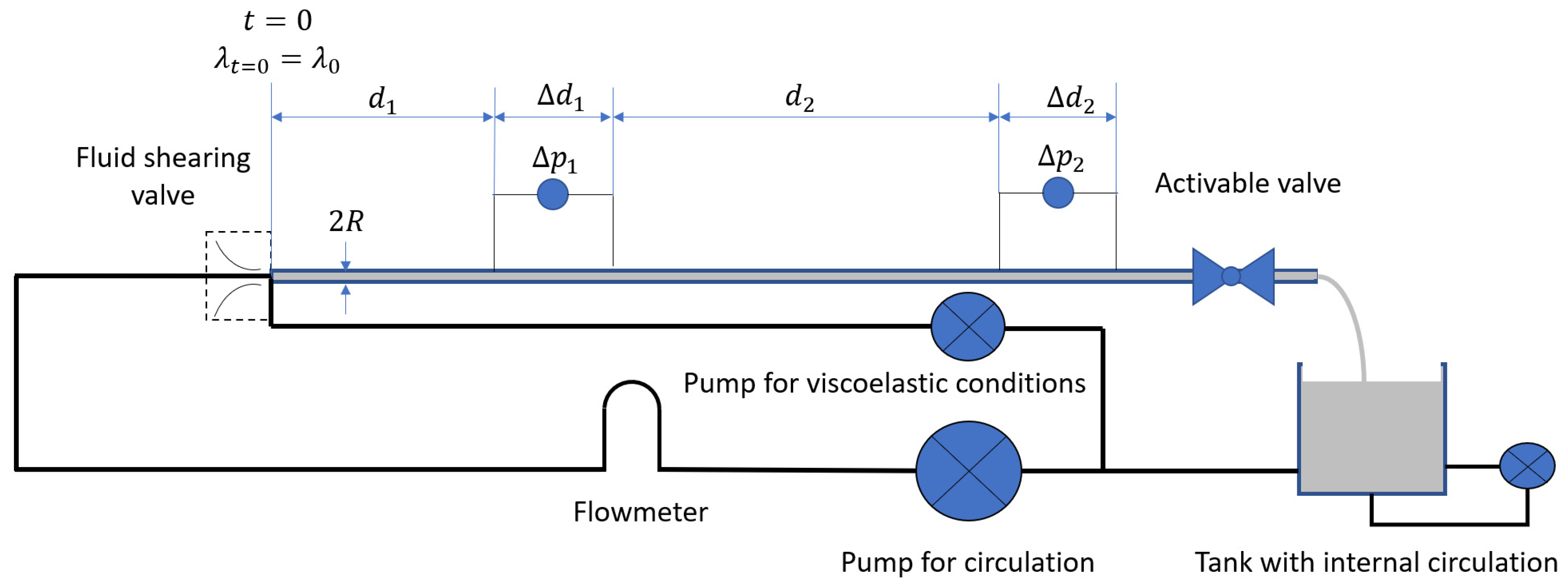
Knowing the viscosity and the shear rate at the wall at any position along the pipe, it is possible to calculate the pressure gradient at each location using Equation (1). In order to apply Equation (7), it is necessary to know the value of the structure parameter at the entrance of the pipe, ${\lambda }_{t=0}$. A possible solution is to ensure that the fluid is completely unstructured when it enters the pipe section. This can be achieved by placing a nozzle or a valve that creates a sufficient pressure drop to fully shear the fluid. In that case, ${\lambda }_{t=0}$ is equal to ${\lambda }_{\infty }$, i.e., the structure parameter is in complete unstructured conditions (see Figure 2).

In this condition, the effective viscosity is:

$$\begin{array}{ll}\eta =& {\eta }_F{\left(\left(1-\left(1+\kappa {\lambda }_{\infty }\right)\frac{\varphi }{{\varphi }_m}\right)e^{-K_1\left({\left(\frac{\dot{\gamma }}{{\dot{\gamma }}_c}\right)}^{n_Q}+1\right)t}\pm \sqrt{\frac{{\eta }_F}{{\eta }_{\infty }}}\frac{{\dot{\gamma }}^{n_Q}}{{\dot{\gamma }}_c^{n_Q}+{\dot{\gamma }}^{n_Q}}\left(e^{-K_1\left({\left(\frac{\dot{\gamma }}{{\dot{\gamma }}_c}\right)}^{n_Q}+1\right)t}-1\right)\right)}^{-2}⟺ \eta \\ & ={\eta }_F{(\left(1-\left(1+\left(\frac{{\varphi }_m}{\varphi }\left(1\pm \sqrt{\frac{{\eta }_F}{{\eta }_{\infty }}}\right)-1\right)\right)\frac{\varphi }{{\varphi }_m}\right)e^{-K_1\left({\left(\frac{\dot{\gamma }}{{\dot{\gamma }}_c}\right)}^{n_Q}+1\right)t}\pm \sqrt{\frac{{\eta }_F}{{\eta }_{\infty }}}\frac{{\dot{\gamma }}^{n_Q}}{{\dot{\gamma }}_c^{n_Q}+{\dot{\gamma }}^{n_Q}}\left(e^{-K_1\left({\left(\frac{\dot{\gamma }}{{\dot{\gamma }}_c}\right)}^{n_Q}+1\right)t}-1\right))}^{-2}⟺ \eta \\ & ={\eta }_F{\left(\pm \sqrt{\frac{{\eta }_F}{{\eta }_{\infty }}}{e}^{-K_1\left({\left(\frac{\dot{\gamma }}{{\dot{\gamma }}_c}\right)}^{n_Q}+1\right)t}\pm \sqrt{\frac{{\eta }_F}{{\eta }_{\infty }}}\frac{{\dot{\gamma }}^{n_Q}}{{\dot{\gamma }}_c^{n_Q}+{\dot{\gamma }}^{n_Q}}\left(e^{-K_1\left({\left(\frac{\dot{\gamma }}{{\dot{\gamma }}_c}\right)}^{n_Q}+1\right)t}-1\right)\right)}^{-2}⟺\eta \\ & ={\eta }_{\infty }{\left(\pm e^{-K_1\left({\left(\frac{\dot{\gamma }}{{\dot{\gamma }}_c}\right)}^{n_Q}+1\right)t}\pm \frac{{\dot{\gamma }}^{n_Q}}{{\dot{\gamma }}_c^{n_Q}+{\dot{\gamma }}^{n_Q}}\left(e^{-K_1\left({\left(\frac{\dot{\gamma }}{{\dot{\gamma }}_c}\right)}^{n_Q}+1\right)t}-1\right)\right)}^{-2},\end{array}$$

(26)

Consequently, by fully shearing the fluid at the entrance of the measuring pipe section, the thixotropic model will depend on only one parameter: $K_1$.

By placing several differential pressure sensors along the measuring pipe section, the impact of thixotropy on pressure losses can be estimated. Several flowrates are utilized, and the measured pressure gradients are used to calibrate the thixotropic Quemada model parameters ${\eta }_{\infty }$, ${\dot{\gamma }}_c$, $n_Q$ and $K_1$. A series of measurement is denoted by $\left\{\left(Q_1,\frac{d{p}_{11}}{ds},\dots , \frac{d{p}_{1k}}{ds} \right),\dots ,\left(Q_m,\frac{d{p}_{m1}}{ds},\dots , \frac{d{p}_{mk}}{ds} \right) \right\}$, where $m$ is the number of flowrates, and $k$ is the number of differential pressure sensors along the measuring pipe. The parameters of the thixotropic Quemada model are found by solving:

$$\left({\eta }_{\infty },{\dot{\gamma }}_c,n_Q,K_1\right)=\underset{{\eta }_{\infty },{\dot{\gamma }}_c,n_Q,{\eta }_F,\kappa ,K_1,\mathsf{\Phi }}{\mathrm{argmin}}\sum _{i=1}^m\sum _{j=1}^k{\left(\frac{d{p}_{ij}}{ds}-f_j\left(Q_i\right)\right)}^2,$$

(27)

where $f_j$ is the function that estimates the pressure gradient at position $j$ along the measuring section of the pipe as a function of the flowrate. This function is simply $f_j=\frac{2{\eta }_{j,Q_i}\dot{\gamma }}{R}$, where ${\eta }_{j,Q_i}$ is calculated using Equation (7) for the position $j$ along the pipe and the flowrate $Q_i$.

The minimization can be solved using a Levenberg–Marquardt method, for instance. Yet, it is necessary to find initial values for ${\eta }_{\infty },{\dot{\gamma }}_c,n_Q{ \mathrm{and} K}_1$ that are not too far from the correct solution.

The further away the measured pressure gradient is from the shearing element, the closer the value is to the one that would correspond to a measurement with no impact of thixotropy. The pressure gradients $\left\{\frac{d{p}_{1k}}{ds},\dots ,\frac{d{p}_{mk}}{ds}\right\}$ are used to estimate ${\eta }_{\infty },{\dot{\gamma }}_c,{ \mathrm{and} n}_Q$ using the method described in the previous section.

It remains to guess the initial values for $K_1$. A flowrate is chosen as well as a pressure gradient is measured as close as possible to the shearing element. This gives:

$${\eta }_{\infty }{\left(\pm e^{-K_1\left({\left(\frac{\dot{\gamma }}{{\dot{\gamma }}_c}\right)}^{n_Q}+1\right)t}\pm \frac{{\dot{\gamma }}^{n_Q}}{{\dot{\gamma }}_c^{n_Q}+{\dot{\gamma }}^{n_Q}}\left(e^{-K_1\left({\left(\frac{\dot{\gamma }}{{\dot{\gamma }}_c}\right)}^{n_Q}+1\right)t}-1\right)\right)}^{-2}=\frac{R}{2\dot{\gamma }}\frac{dp}{ds},$$

(28)

Using the estimated values of ${\eta }_{\infty },{\dot{\gamma }}_c,{ \mathrm{and}n}_Q$, the value of $t$ estimated with Equation (25) and the value of $\dot{\gamma }$ at the wall obtained from the fluid velocity calculated using steady-state conditions, Equation (28) is only a function of $K_1$. The equation is solved numerically using a Newton–Raphson method.

Equipped with the initial guess, the minimization problem described by Equation (27) is solved, and the four parameters ${\eta }_{\infty },{\dot{\gamma }}_c,n_Q,{ \mathrm{and} K}_1$ are estimated.

5. Calibration of the Viscoelastic Properties

To create conditions that are relevant for the estimation of the viscoelastic properties of a fluid, i.e., its elastic constants, the circulation in the flow loop is stopped, and then new fluid is slowly pushed into the measuring pipe section to allow estimating the elastic and viscous response of the fluid.

It should be noted that when the measuring pipe section has a return by gravity to the tank, even though the pump is stopped, the flow may continue for some time, simply because the tube tends to empty itself. To stop the flow precisely, it is necessary to have an activable valve that is closed just after the pump has stopped. Also, to have a slow movement of the fluid during the period for which both elastic and viscous behaviors are visible, a different injection system than the one used for full circulation may be used. This low flowrate injection system bypasses the fluid-shearing valve (see Figure 3).

When the fluid movement is reinstated after a resting period, the value of the structure parameter corresponds to the fully structured value, i.e., ${\lambda }_0$. When introducing its value from Equation (9) into the Quemada thixotropic model in Equation (7), the viscous behavior of the fluid is described by:

$$\begin{array}{ll}\eta =& {\eta }_F{\left(\left(1-\left(1+\kappa {\lambda }_{\infty }\right)\frac{\varphi }{{\varphi }_m}\right)e^{-K_1\left({\left(\frac{\dot{\gamma }}{{\dot{\gamma }}_c}\right)}^{n_Q}+1\right)t}\pm \sqrt{\frac{{\eta }_F}{{\eta }_{\infty }}}\frac{{\dot{\gamma }}^{n_Q}}{{\dot{\gamma }}_c^{n_Q}+{\dot{\gamma }}^{n_Q}}\left(e^{-K_1\left({\left(\frac{\dot{\gamma }}{{\dot{\gamma }}_c}\right)}^{n_Q}+1\right)t}-1\right)\right)}^{-2}⟺ \eta \\ & ={\eta }_F{(\left(1-\left(1+\left(\frac{{\varphi }_m}{\varphi }\left(1\pm \sqrt{\frac{{\eta }_F}{{\eta }_{\infty }}}\right)-1\right)\right)\frac{\varphi }{{\varphi }_m}\right)e^{-K_1\left({\left(\frac{\dot{\gamma }}{{\dot{\gamma }}_c}\right)}^{n_Q}+1\right)t}\pm \sqrt{\frac{{\eta }_F}{{\eta }_{\infty }}}\frac{{\dot{\gamma }}^{n_Q}}{{\dot{\gamma }}_c^{n_Q}+{\dot{\gamma }}^{n_Q}}\left(e^{-K_1\left({\left(\frac{\dot{\gamma }}{{\dot{\gamma }}_c}\right)}^{n_Q}+1\right)t}-1\right))}^{-2}⟺ \eta \\ & ={\eta }_F{\left(\pm \sqrt{\frac{{\eta }_F}{{\eta }_0}}{e}^{-K_1\left({\left(\frac{\dot{\gamma }}{{\dot{\gamma }}_c}\right)}^{n_Q}+1\right)t}\pm \sqrt{\frac{{\eta }_F}{{\eta }_{\infty }}}\frac{{\dot{\gamma }}^{n_Q}}{{\dot{\gamma }}_c^{n_Q}+{\dot{\gamma }}^{n_Q}}\left(e^{-K_1\left({\left(\frac{\dot{\gamma }}{{\dot{\gamma }}_c}\right)}^{n_Q}+1\right)t}-1\right)\right)}^{-2}⟺\eta \\ & ={\eta }_{\infty }{\left(\pm \sqrt{\frac{{\eta }_{\infty }}{{\eta }_0}}{e}^{-K_1\left({\left(\frac{\dot{\gamma }}{{\dot{\gamma }}_c}\right)}^{n_Q}+1\right)t}\pm \frac{{\dot{\gamma }}^{n_Q}}{{\dot{\gamma }}_c^{n_Q}+{\dot{\gamma }}^{n_Q}}\left(e^{-K_1\left({\left(\frac{\dot{\gamma }}{{\dot{\gamma }}_c}\right)}^{n_Q}+1\right)t}-1\right)\right)}^{-2},\end{array}$$

(29)

and since it was assumed that $\chi =\sqrt{\frac{{\eta }_{\infty }}{{\eta }_0}}$ can be considered null, the result is:

$$\eta ={\eta }_{\infty }{\left(\frac{{\dot{\gamma }}^{n_Q}}{{\dot{\gamma }}_c^{n_Q}+{\dot{\gamma }}^{n_Q}}\left(1-e^{-K_1\left({\left(\frac{\dot{\gamma }}{{\dot{\gamma }}_c}\right)}^{n_Q}+1\right)t}\right)\right)}^{-2},$$

(30)

Now, the structure parameter is evaluated using the initial condition:

$$\begin{array}{ll}\lambda \left(t\right)=& \frac{\left(\frac{1}{\kappa }\left(\frac{1}{\mathsf{\Phi }}\left(1\pm \sqrt{\frac{{\eta }_F}{{\eta }_{\infty }}}\right)-1\right){\left(\frac{\dot{\gamma }}{{\dot{\gamma }}_c}\right)}^n+{\lambda }_0\right)}{{\left(\frac{\dot{\gamma }}{{\dot{\gamma }}_c}\right)}^n+1}\\ & \hspace{1em}\hspace{1em}\hspace{1em}+\left(\frac{1}{\kappa }\left(\frac{1}{\mathsf{\Phi }}\left(1\pm \sqrt{\frac{{\eta }_F}{{\eta }_0}}\right)-1\right)-\frac{\left(\frac{1}{\kappa }\left(\frac{1}{\mathsf{\Phi }}\left(1\pm \sqrt{\frac{{\eta }_F}{{\eta }_{\infty }}}\right)-1\right){\left(\frac{\dot{\gamma }}{{\dot{\gamma }}_c}\right)}^n+{\lambda }_0\right)}{{\left(\frac{\dot{\gamma }}{{\dot{\gamma }}_c}\right)}^n+1}\right)e^{-K_1\left({\left(\frac{\dot{\gamma }}{{\dot{\gamma }}_c}\right)}^n+1\right)t},\end{array}$$

(31)

And considering that ${\eta }_0$ is supposed to tend to infinity, $\sqrt{\frac{{\eta }_F}{{\eta }_0}}\to 0$. Equation (31) is simplified to:

$$\begin{array}{ll}\lambda \left(t\right)=& \frac{\left(\frac{1}{\kappa }\left(\frac{1}{\mathsf{\Phi }}\left(1\pm \sqrt{\frac{{\eta }_F}{{\eta }_{\infty }}}\right)-1\right){\left(\frac{\dot{\gamma }}{{\dot{\gamma }}_c}\right)}^n+{\lambda }_0\right)}{{\left(\frac{\dot{\gamma }}{{\dot{\gamma }}_c}\right)}^n+1}\\ & \hspace{1em}\hspace{1em}\hspace{1em}+\left(\frac{1}{\kappa }\left(\frac{1}{\mathsf{\Phi }}-1\right)-\frac{\left(\frac{1}{\kappa }\left(\frac{1}{\mathsf{\Phi }}\left(1\pm \sqrt{\frac{{\eta }_F}{{\eta }_{\infty }}}\right)-1\right){\left(\frac{\dot{\gamma }}{{\dot{\gamma }}_c}\right)}^n+{\lambda }_0\right)}{{\left(\frac{\dot{\gamma }}{{\dot{\gamma }}_c}\right)}^n+1}\right)e^{-K_1\left({\left(\frac{\dot{\gamma }}{{\dot{\gamma }}_c}\right)}^n+1\right)t},\end{array}$$

(32)

It should be noted that $E_0$ in Equation (13) is constant when the fluid movement starts. However, its value changes during the gelation period. From the results showing that the stress overshoot is a logarithmic function of the gelling time, it seems reasonable to suppose that $E_0$ also is a logarithmic function of the gel duration:

$$E_0\left(t_{gel}\right)=E_0\left(t_{{gel}_1}\right)+\left(E_0\left(t_{{gel}_2}\right)-E_0\left(t_{{gel}_1}\right)\right)\frac{\ln t_{gel}-\ln t_{{gel}_1}}{\ln t_{{gel}_2}-\ln t_{{gel}_1}}, \forall t_{gel}\ge t_{{gel}_0},$$

(33)

Then, it is possible to calculate Equation (11) by introducing the expressions of viscosity, $\eta$, from Equation (30), the expression of the structure parameter, $\lambda$, from Equation (32) and the expression of the initial elastic modulus before fluid movement, $E_0$, using Equation (33). This provides the time evolution of the shear stress as a function of time and shear rate $\dot{\gamma }$.

Even though it was shown that, in non-steady-state conditions, the relationship in Equation (1) is not true [17], when working with very small flowrates and accelerations, the influence of inertial terms is negligeable, and Equation (1) is nevertheless an acceptable approximation of the relationship between shear stress and pressure gradient. Therefore, it is possible to observe the shear stress at flow initiation of the thixo-elastic fluid by monitoring the pressure gradient. Note that the measurements at the distributed differential pressure sensors are identical because the shear history, from the moment the fluid has stopped, is identical along the pipe because of the fluid incompressibility hypothesis.

As it is necessary to control precisely the acceleration, the velocity and the volume injected at very low values and since the total volume that shall be pumped under these conditions is relatively small, the pump used for thixo-elastic measurements can be replaced by a motorized syringe (see Figure 4).

The thixo-elastic testing procedure is the following:

• The circulation is stopped.
• The outlet valve is closed.
• The fluid is left to rest for a given time.
• The outlet valve is opened.
• The syringe is activated with a low acceleration to reach a low velocity.

This procedure is repeated two times with different rest durations. The two resulting pressure gradient time profiles are then used to calibrate the missing parameters $\kappa$, $\mathsf{\Phi }$, ${\eta }_F$, $E_0\left(t_{{gel}_1}\right)$ and $E_0\left(t_{{gel}_2}\right)$. This leads to the following minimization problem:

$$\left(\kappa ,\mathsf{\Phi },{\eta }_F, E_0\left(t_{{gel}_1}\right),E_0\left(t_{{gel}_2}\right)\right)=\underset{\kappa ,\mathsf{\Phi },{\eta }_F, E_0\left(t_{{\mathit{gel}}_1}\right),E_0\left(t_{{\mathit{gel}}_2}\right)}{\mathrm{argmin}}\sum _{i=1}^2\sum _{j=1}^{k_i}{\left(\frac{d{p}_{ij}}{ds}-\frac{2\tau \left(t_{ij}\right)}{R}\right)}^2,$$

(34)

where $i$ denotes the index of the procedure, $k_i$ is the number of measurements acquired during the test procedure $i$, $\frac{d{p}_{ij}}{ds}$ is the pressure gradient measured during the procedure $i$ at the time step $j$, and $\tau \left(t_{ij}\right)$ is the shear stress evaluated using Equation (11) at time $t_{ij}$. Note that the shear rate at the wall is estimated using the transient model described by Equation (17).

The first time the minimization needs to be solved, it is not easy to guess initial values that are close to the absolute minimum, which rules out the use of typical steepest descent or gradient minimization algorithms. Instead, a particle swarm optimization method is used to find the global minimum [23,24]. However, this method is slow and computer-intensive. After the first minimization has been performed, the obtained values are used as the initial guess for a minimization algorithm such as the Levenberg–Marquardt, which is much faster. Yet, the fluid characteristics may change through time, and it is therefore necessary to check if another global minimum can be found. This is achieved by running regularly the particle swarm optimization algorithm instead of the Levenberg–Marquardt algorithm.

6. Discussion

The impact of thixotropy and visco-elasticity of non-Newtonian fluids was used to propose a different design for a pipe rheometer. The new design allows making measurements in well-defined conditions. These conditions were chosen to facilitate the calibration of the various parameters of the model.

As a result of this analysis, the new pipe rheometer is equipped with two different pressure sensors that measure the pressure drop over a short distance, differently from the classical pipe rheometers for which the ports of the differential pressure sensor are usually close to each end of a long tube. This design change is essential because, when circulating thixotropic fluids, the pressure gradient is different at various positions along the pipe section. Furthermore, a shearing element was introduced at the start of the measuring pipe section. This element is also crucial to ensure that the structure parameter of the thixotropic fluid is known at the entrance of the section. By imposing a structure parameter equal to the one when the shear rate tends to infinity, several simplifications are possible for the thixotropic Quemada model, thereby thereby leading to a reduction in the dependence of the results on a single parameter relating to thixotropy, $K_1$. This in turn facilitates the calibration of the thixotropic Quemada model, as only four parameters are calibrated at that stage: ${\eta }_{\infty },{\dot{\gamma }}_c,n_Q,{ \mathrm{and} K}_1$. By changing the flowrate several times and recording the pressure gradients at two positions along the measuring section, a method was described to calibrate efficiently these four parameters.

To address the problem of finding the remaining thixo-elastic properties of the fluid, the new design includes a valve to close the outlet of the measuring section in order to ensure that there is no flow during the gelling period. Also, a syringe is used to obtain a precise control of the flow initiation after gelling. By repeating the procedure two times, it is then possible to calibrate five additional parameters of the thixo-elastic shear-thinning fluid model: $\kappa ,\mathsf{\Phi },{\eta }_F, E_0\left(t_{{gel}_1}\right),{ \mathrm{and} E}_0\left(t_{{gel}_2}\right)$. The calibration method is computer-intensive, at least for the first time or when a new fluid is run into the pipe rheometer. After the initial calibration has been performed, a lighter minimization algorithm can be used.

The proposed method relies on the fact that the fluid and the system are incompressible. To ensure that the system does not introduce any compressibility sources, all parts must be made of stiff materials like steel or glass. Rubber or elastomer hoses shall not be used. It may be more difficult to ensure that the fluid is incompressible, as sometime the liquid may contain bubbles. To reduce the impact of bubbles on the measurements, it may be useful to terminate the measuring section with a controllable valve that provides a back pressure. With a sufficient back pressure, the bubble size may be reduced to a very small volume, and therefore, the incompressibility hypothesis may be better respected.

Yet, the described design and method have some possible sources of uncertainties. The first one is linked to the effect of the shearing element. The flow behind it is not fully developed at some unknown distance. This can impact the development of the structure parameter of the fluid in this region and, therefore, influence the accuracy of the calibration of $K_1$. Second, it is hypothesized that the elastic modulus at zero shear rate, $E_0$, is a logarithm function of the gelling time. Even though this seems to be a reasonable hypothesis based on previous observations, this supposition was not verified. Third, it should be noted that this study only addressed the case of the Quemada shear-thinning rheological behavior for which the viscosity at zero shear rate tends to a very large value, i.e., ${\eta }_0\to \infty$. It is possible that the same principles can be applied to shear-thickening fluids and to fluid with a finite ${\eta }_0$, but that was not analyzed.

Despite the above-mentioned limitations, the described design and calibration method allow obtaining the nine parameters of a thixo-elastic shear-thinning Quemada rheological behavior. This enables to use such an advanced model for very dynamic conditions within which transient circulations alternate with resting periods.

7. Conclusions

Measuring the rheological properties of complex non-Newtonian fluids that exhibit thixotropic and viscoelastic effects is a difficult task. This paper investigated how a pipe rheometer can manage that challenge.

Here are the main results:

• Having a large distance between the ports of the differential pressure sensor along the measuring pipe section implies that the measurements are biased when circulating a thixotropic fluid.
• Utilizing a short distance between the two ports of the differential pressure sensor and two differential pressure measurements at a sufficient distance from each other allows assessing some of the thixotropic properties of the circulated fluid, considering that the initial shear conditions are imposed at the start of the pipe section. This can be achieved by using a fluid-shearing element.
• By closing the outlet of the pipe section with a valve during a resting period and then opening that valve and injecting fluid at low velocity, it is possible to acquire a characteristic pressure curve that can be used to calibrate the remaining thixotropic parameters and the elastic properties of the gelled fluid.

The proposed design is rather different from existing pipe rheometer solutions. The new design is justified by the analysis of the physical phenomena that influence the pressure gradient when circulating a viscoelastic and thixotropic fluid. It should allow obtaining more precise estimations of the steady-state properties of non-Newtonian fluids and, at the same time, provide the opportunity to acquire all the parameters that describe the thixo-elastic behavior of complex fluids.