The BMP model is described by the following equations [
21]:
where
is the upper-convected derivative of the stress tensor,
is the symmetric part of the rate of the strain tensor,
is the fluidity (inverse of the shear viscosity
),
is the zero-shear-rate fluidity,
is the fluidity at high shear rates,
is the shear modulus,
is the structural characteristic time, and
is a kinetic constant related to structure modification. The upper-convected derivative of the stress tensor is
where
is the velocity gradient tensor. Equations (1) and (2) reduce to the upper-convected Maxwell model when
. These equations express that the nonlinear viscoelastic processes contained in the Maxwell equation are coupled with an equation written in terms of the fluidity, which is itself a kinetic equation with a characteristic time related to structure formation
and a destruction term related to structure modification with a kinetic constant
proportional to the dissipation. Under simple shear flow, the above equations reduce to
where
is the shear rate and the nonlinear terms in Equation (3) are not considered, which implies that the normal stresses generated under flow are negligible. In steady state, both Equations (4) and (5) can be reduced to provide
Equation (6) predicts shear-thinning behavior when
, shear-thickening behavior when
, and Newtonian behavior when
. A plateau region is predicted in the limits of very low and very high shear rates, with a power-law behavior at the intermediate shear rates. In addition, a stress plateau is predicted when
. This implies a constant stress in the limit as the shear rate approaches zero. An apparent yield is predicted for very small values of
. The physical meaning of Equation (6) can be revealed if it is written in terms of the non-dimensional dissipation, as follows:
Upon increasing dissipation
, while for decreasing dissipation
. From Equation (6), the plateau stress can be calculated when
in the region of very small shear rates. This results in
The three independent parameters in Equation (9) can be evaluated from the flow curve itself in the form of the viscosity versus the shear rate. The fluidity at low strain rates
(inverse viscosity) is extracted from the first Newtonian plateau at vanishing shear rates, and the fluidity at an infinite shear rate
corresponds to the plateau at high shear rates. When the plateau stress is approached, the viscosity tends to a slope of
in a log–log plot. The usual form from which the plateau stress is evaluated considers the plateau that is exhibited as the shear rate tends to zero in a plot of the log stress versus log shear rate. In this context, the model does not contain fitting parameters. We can calculate the fluidity at the plateau stress by setting
; this provides
According to the model presented here, the pores are considered as capillaries with different diameters. The change in capillary radius is taken into account by modifying the tortuosity along the flow trajectories, and several results are shown in which changes in tortuosity or fractal dimensions are considered. Although transient flow exists in a real porous medium (i.e., complex expansion–contraction trajectories), in this model the change in geometry which modifies trajectories is considered as a change in tortuosity and a change in fractal dimensions. In other words, following the averaging procedures considered in the present model, the overall flow may be considered steady; however, locally it is intrinsically unsteady. This transient state is taken into account by the variation in thew tortuosity or fractal dimensions of the porous medium in time scales shorter than that of the global averaged macroscopic flow.
2.1. Calculation of Mobility
The procedure to calculate the mobility in a complex fluid is outlined in (the appendix of reference [
6]). A momentum balance on a differential element in cylindrical geometry leads to a relationship between the shear stress and the pressure gradient; in this case, the shear stress at wall in tortuous capillaries is provided by [
22,
23].
Following the fractal scaling method, the wall shear stress is [
6]
where
is the fractal dimension describing the tortuous length of the capillary. Darcy’s law may then be written in terms of the non-Newtonian mobility as follows:
where
As the capillaries in porous media are tortuous, the total shear stress in Equation (12) at all capillary walls is related to the fractal dimensions
and
, microstructual parameters, and pressure gradient (see [
6]). The resulting effective permeability is
The Newtonian permeability may be obtained as a particular case when
,
(Poiseuille’s law), yielding
In straight capillaries,
; therefore, we can obtain
This equation agrees with those of the current literature for Newtonian fluids. We obtained an analytical result for the permeability provided
can be calculated [
6]. This may be achieved assuming that the fluidity in the pore/capillary attains a minimum in the center of the geometry and reaches a maximum at the walls, i.e.,
Accordingly, the fluidity attains its minimum at the capillary center
, that is,
, and its maximum at the walls
,
. The fluidity at the wall requires the calculation of the wall stress according to Equation (11). Thus, the final result is [
6]
When
, next to the capillary center, the permeability tends to the Newtonian constant value provided by Equation (16). Near the wall,
tends to a maximum value and the permeability diminishes asymptotically to another constant value as a function of the maximum fluidity. By defining
Equation (19) can be expressed as
Clearly, within the limit
the permeability is constant, providing
In straight capillaries
,
which agrees with Equation (17). The non-Newtonian fluid mobility in Equation (14) becomes
which reduces to the Newtonian mobility
where
is the fluidity of the Newtonian fluid, while the mobility ratio becomes
In Equation (26), the ratio is
The limits of Equation (26) consider expressions at low and high stresses; in the low range,
and
. At the upper stress limit,
, and hence
In
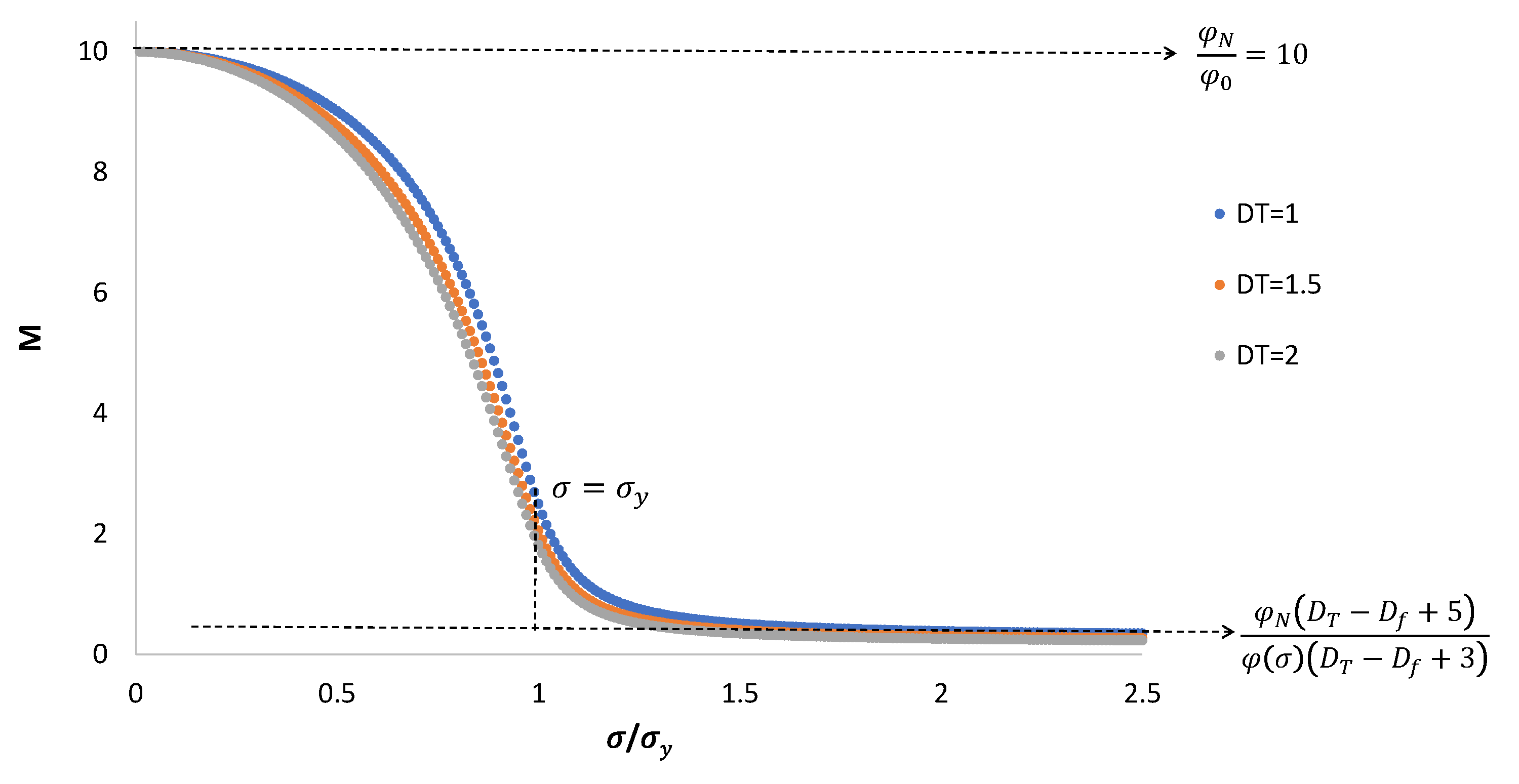
Figure 1, a plot of the normalized fluidity as a function of the stress normalized by the yield stress is disclosed. We consider a Newtonian fluid with viscosity ten times smaller than that of the non-Newtonian fluid at small stresses. As the stress increases, the fluidity of the non-Newtonian fluid increases as well, overtaking that of the Newtonian fluid. In
Figure 2, the mobility ratio is plotted with the applied stress.
We define the following relative permeabilities:
where
is the relative permeability of fluid
i and
is the characteristic permeability of fluid
i.
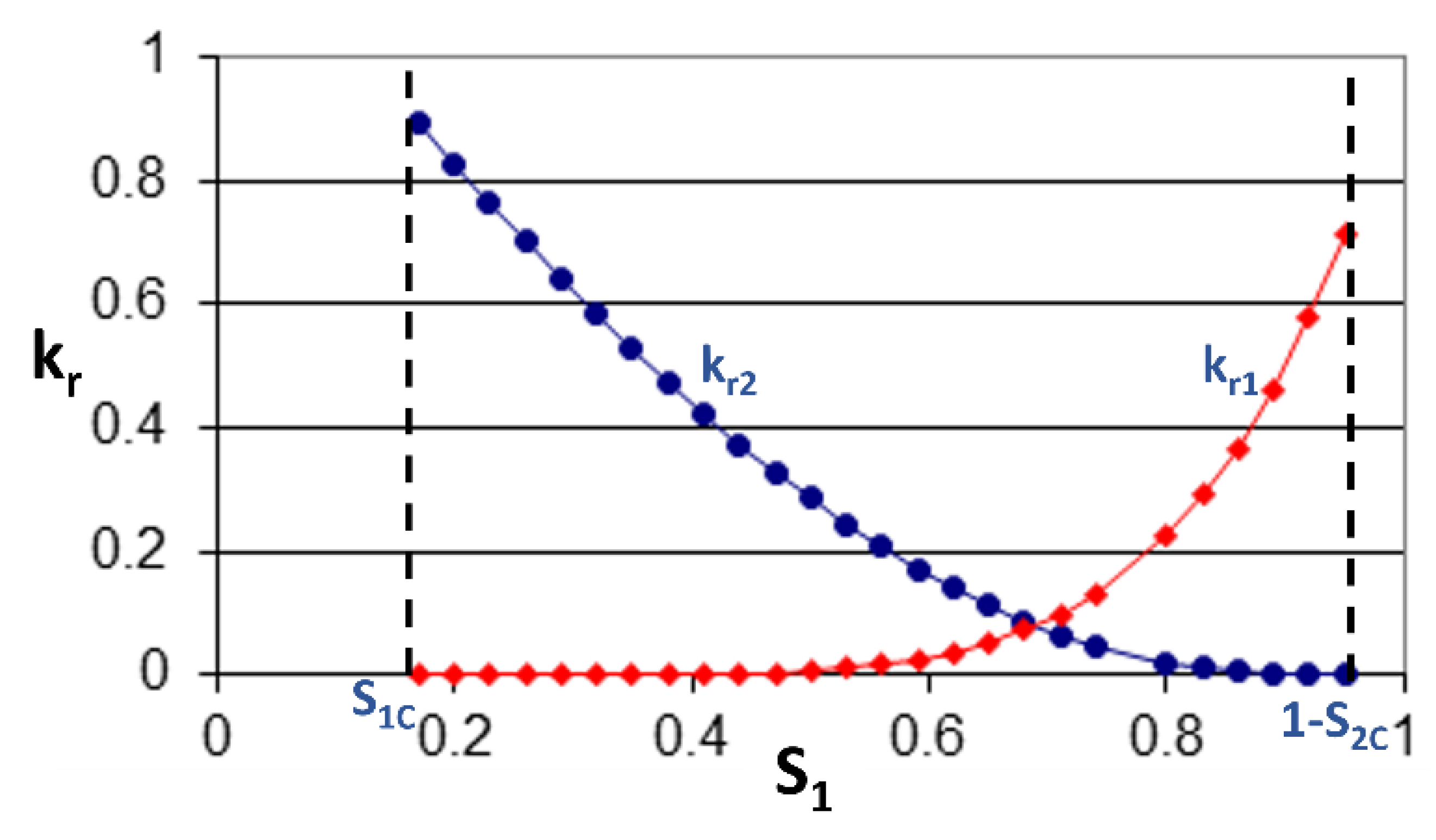
Figure 3 shows the variation of the relative permeabilities as a function of the saturation.
Saturation limits are
for Fluid 1 such that
is the maximum saturation of Fluid 1 and the minimum saturation of Fluid 2.
Figure 3 shows that there is a quadratic dependence of the relative permeability on the saturation, and therefore the following relations represent this variation:
from the material balance for the two fluids, namely,
Upon substitution of the above equations for those of Darcy’s law for each fluid provides the following displacement velocities in the porous medium:
considering that the capillary pressure depends only on saturation
and the flow fractions are defined as follows:
where
represents the sum of the flow rate fractions, as the flow area is the same for both fluids. Deriving Equation (37) with respect to
x and solving for the pressure gradients in Equations (35) and (36), upon substitution we obtain
Using Equations (32) and (33) and the definition of the mobility ratio
, we obtain
which can be expressed as
where
From the mass balance
the following equation is obtained:
2.1.1. The Buckley–Leverett Equation
Neglecting the capillary forces, Equation (46) reduces to
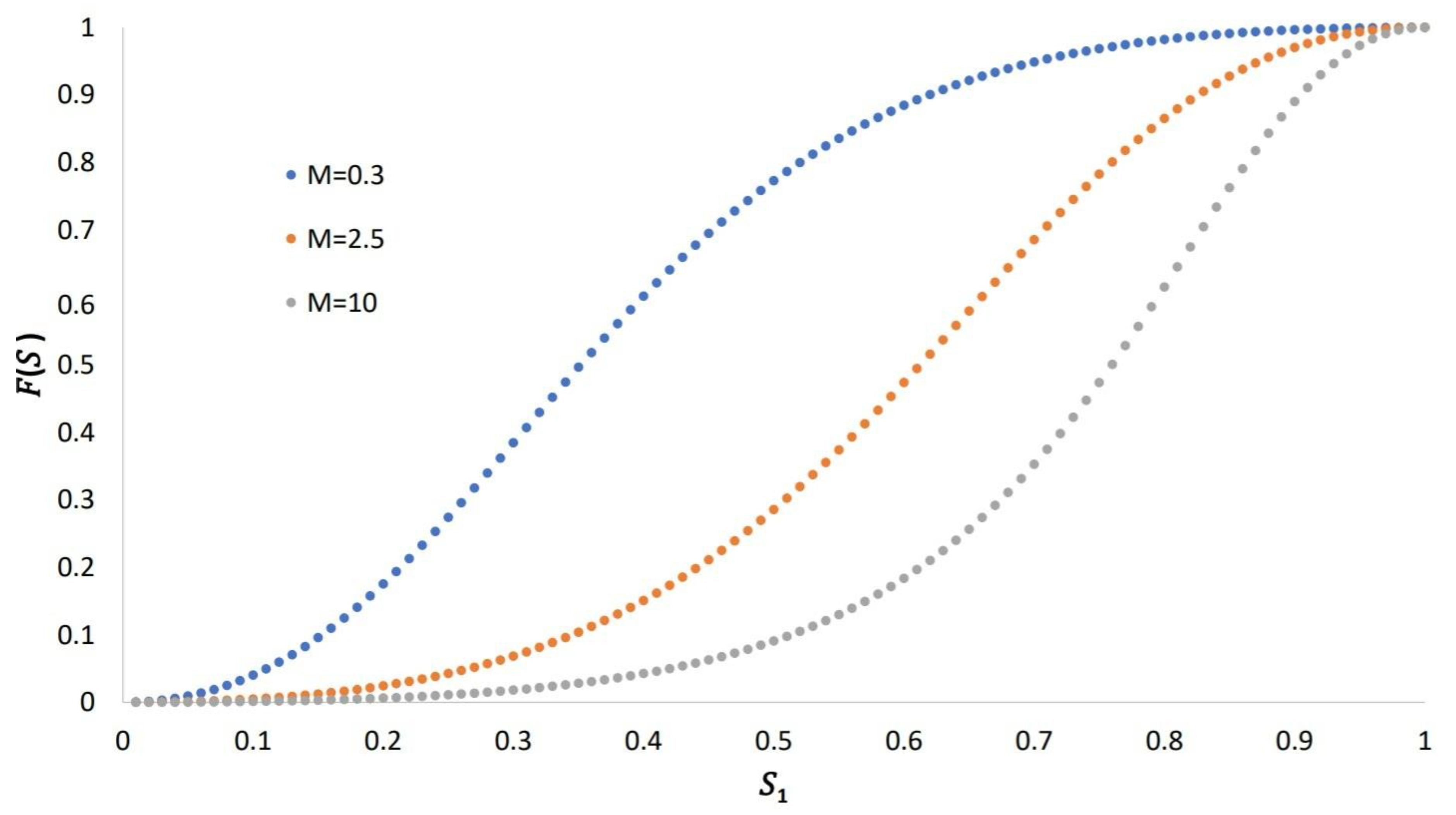
A plot of the flow fraction
as a function of the saturation
S for the three mobility ratios considering
is shown in
Figure 4.
Next, we make Equation (46) non-dimensional by defining the variables
and
. Dropping the sub-index, we can express Equation (46) as follows:
where
S refers to the saturation of Fluid 1. Up to first order in the derivatives and small capillary pressure contributions, Equation (48) leads to
The Buckley–Leverett problem does not consider capillary effects:
The material derivative of S in one dimension is
Comparing Equations (50) and (51), we obtain
where
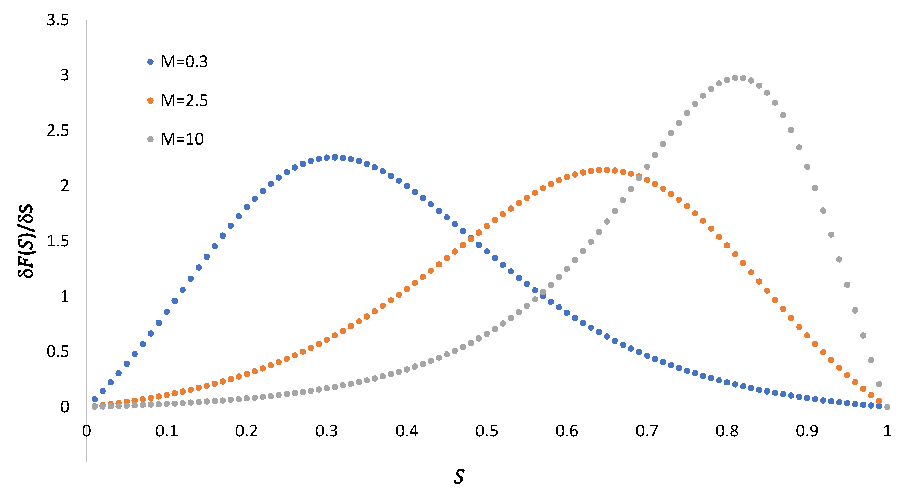
In
Figure 5, we plot Equation (53)
for the three mobility ratios.
We can integrate Equation (52) as follows:
Because the function
is not single-valued, the Buckley–Leverett analysis includes the calculation of the tangent to the flux function
and the presence of a shock. The tangent condition reads
A unique root of Equation (55) is obtained, namely,
which is the abscise of the point of intersection of the tangent and the function
. The slope of the tangent is found from the condition
and the mean saturation
is found if
, namely,
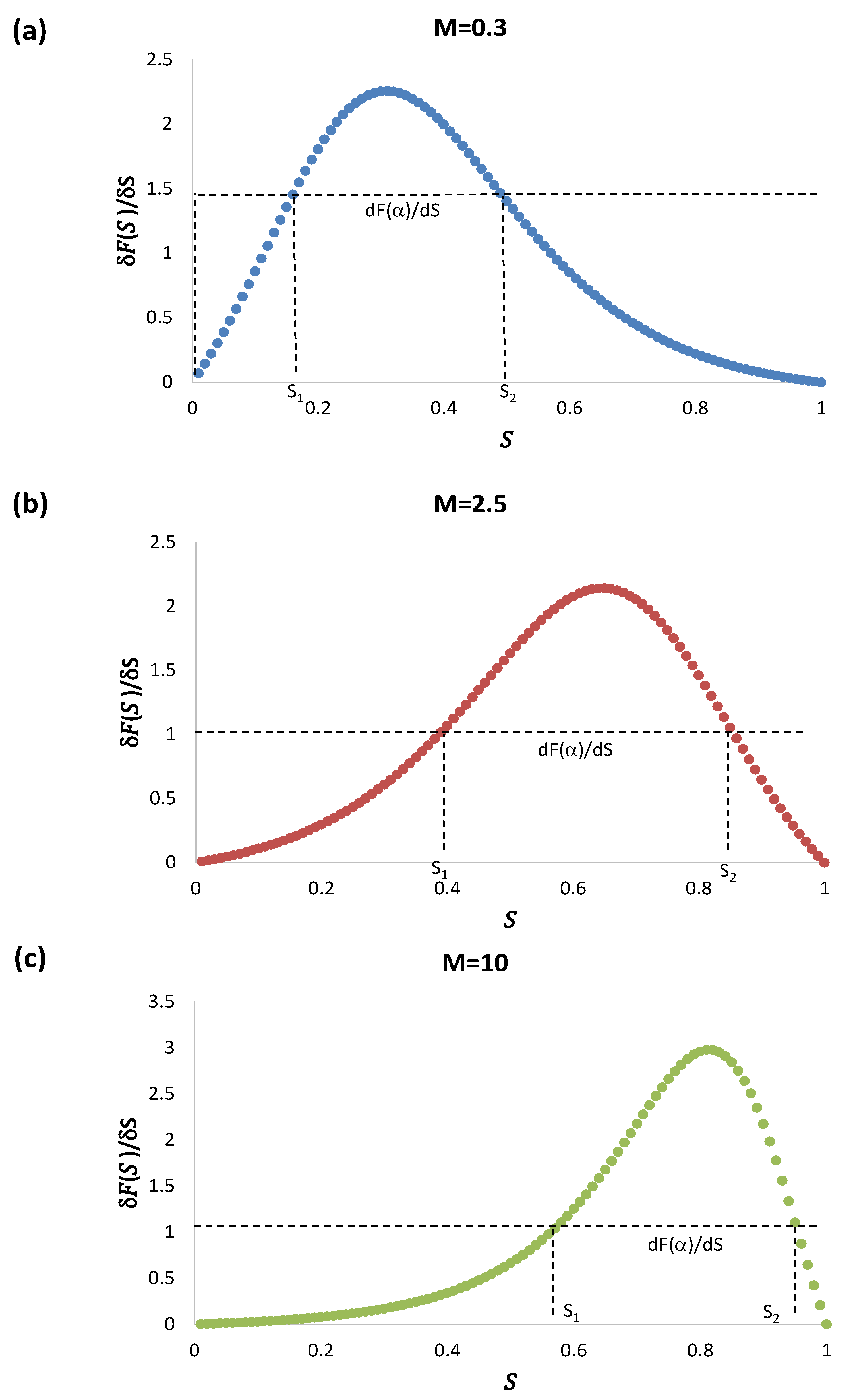
In
Figure 6a–c, we plot the flux function
and its derivative together with the tangent to locate the intersection point
.
As the mobility ratio increases, the intersection point of the tangent and the function
has ordinate
approaching one as well as
see
Figure 7, and hence the slope tends to
; see
Table 1.
In
Figure 1 and
Figure 2, it is clear that for low pressure gradients (namely, small stresses) the fluidity of the displacing fluid is small and the ratio of its fluidity with the fluidity of the Newtonian oil is large
. The plateau stress of the micellar fluid coincides with that of the oil, with a mobility ratio around 2. For high pressure gradients, the fluidity of the non-Newtonian fluid is large (close to that of water), even larger than that of the oil. In this case the displacing action of the displacing fluid decreases, which is convenient for actual enhanced oil recovery operations. It is worth mentioning that the viscosity of the displacing fluid should be properly adjusted along with the applied pressure gradient in order to provide the optimal oil displacement. This is one of the advantages of a complex non-Newtonian fluid, which provides multiple options for actual oil operations.
The equal area criterion is used to specify the value at which the shock should occur, namely,
where
denotes the ordinate at which the equal area criterion holds. Equation (59) is an illustration of the mean value theorem of integrals. In fact, if
and
, Equation (59) is satisfied. Therefore, the shock occurs at a value of the saturation equal to
and ordinate
, which is the speed of propagation according to Equation (52). In the
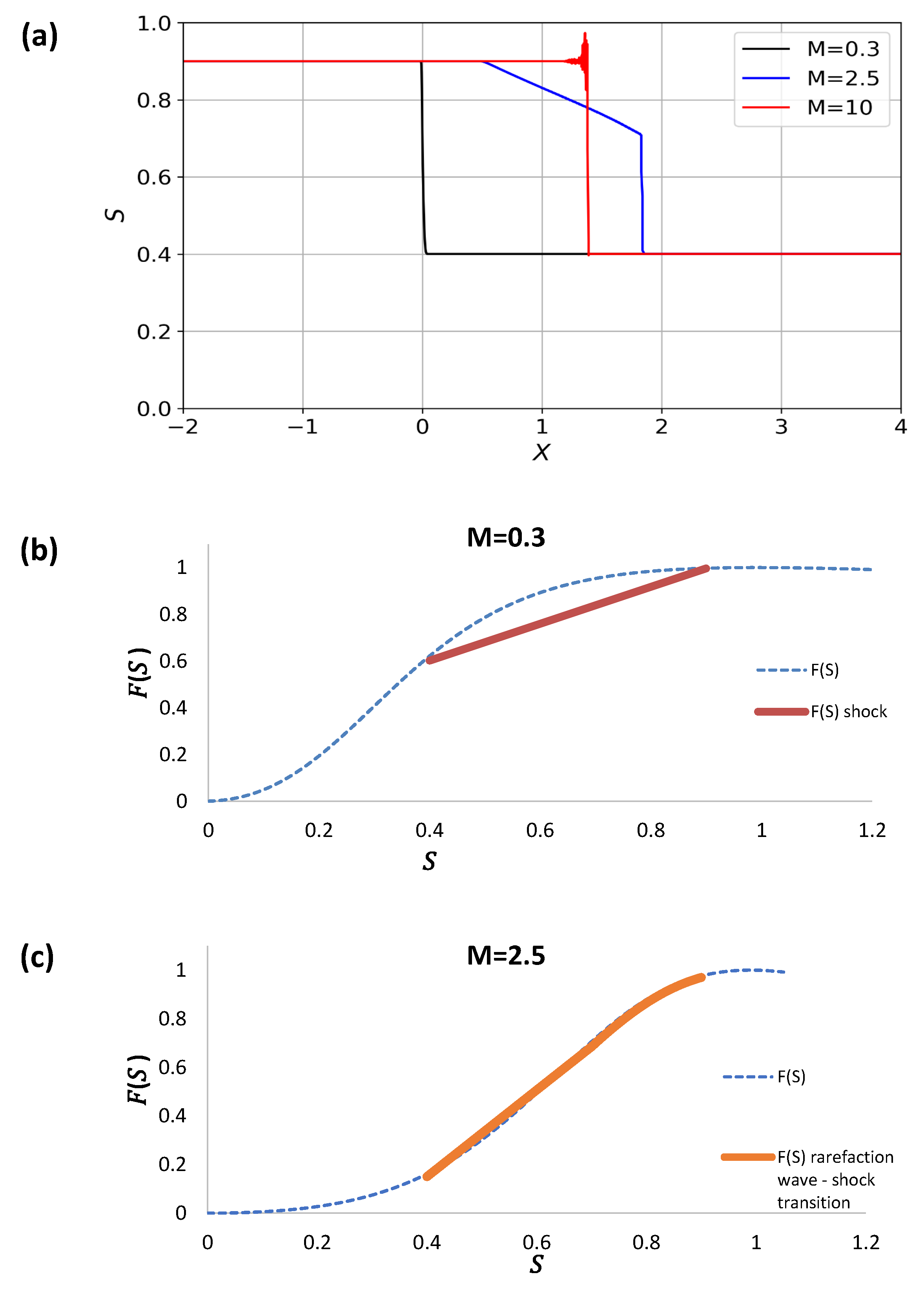
Figure 8a–c, the saturation is plotted as a function of the propagation speed for the three mobilities.
Figure 9a–c depict the speed of propagation of the shock profile as the mobility changes. The speed is higher as the mobility ratio decreases. This effect is expected, as the viscosity of the displacing non-Newtonian fluid is larger for
. For higher pressure gradients the displacing fluid viscosity diminishes, allowing for larger propagation speeds. In
Figure 10, the saturation is plotted with the propagation speed for the three fronts, exhibiting the effect of diminishing the viscosity of the non-Newtonian pushing fluid for large pressure gradients.
To further analyse the shock profiles, let
be the saturation value to the left of the shock and let
the value of the saturation to the right of the shock; moreover, let the boundary conditions be
The slope just before and after the shock corresponds to the Rankine–Hugoniot condition:
if
. Applying the boundary conditions, we obtain
which corresponds to the tangent condition. Furthermore, applying the Oleinik entropy condition
if
,
and
. Hence, the criterion of equal areas is sufficient to define the shock location according to the Oleinik criterion.
2.1.2. Capillary Pressure
Here, we consider the model by Hassanizadeh and Gray, in which the capillary pressure can be described according to the following expression:
where
is the static capillary pressure and
is a characteristic time. In this case, and considering that the capillary pressure in equilibrium is generally a decreasing function of saturation
, Equation (46) becomes:
We discuss an extension to the B-L equation which includes the third-order mixed derivatives term and models the capillary pressure. Travelling wave solutions exist in the extended model. The speed of the shock, , and are related through the Rankine–Hugoniot (RH) condition Equation (62). Experiments in two-phase flow in porous media reveal complex infiltration profiles with overshoots (i.e., non-monotone profiles). Solutions with the second derivative term exist if , , and satisfy the RH and Oleinik entropy conditions. In the limit , traveling waves converge to the shock .
If
, then a weak solution is composed of a rarefaction wave in the region where
and a shock that spans the range
. Focusing on the relation of
and
, we establish the existence of the function
where
is defined through the equal area criterion
in such a way that Equation (66) may possess a shock wave solution in which
in which case
is a bifurcation parameter when
. For the case in which
, the criterion
is not fulfilled, and new types of shock waves are admissible.
With as defined above, we establish the existence of a function defined for such that Equation (66) has a travelling wave solution with if and only if .
The solution of Equation (66) for various cases is illustrated in the following plots; here, .
A Fortran numerical code was developed using the finite difference scheme proposed by [
14]. This code was used to solve the model governing equation (see Equation (5.1) in [
14]). With same parameters used by them, the computations were performed on the interval
, with
for the rarefaction and rarefaction-under-compressive shock solutions and
in other cases. All solutions are shown at time
and with
. The numerical code was validated by comparing the cases reported by [
14]. The results showed that the present code qualitatively reproduces the same results as shown in their figures.


 ,
, 


