Single-Mode Solutions for Convection and Double-Diffusive Convection in Porous Media

Abstract

This work employs single-mode equations to study convection and double-diffusive convection in a porous medium where the Darcy law provides large-scale damping. We first consider thermal convection with salinity as a passive scalar. The single-mode solutions resembling steady convection rolls reproduce the qualitative behavior of root-mean-square and mean temperature profiles of time-dependent states at high Rayleigh numbers from direct numerical simulations (DNS). We also show that the single-mode solutions are consistent with the heat-exchanger model that describes well the mean temperature gradient in the interior. The Nusselt number predicted from the single-mode solutions exhibits a scaling law with Rayleigh number close to that followed by exact 2D steady convection rolls, although large aspect ratio DNS results indicate a faster increase. However, the single-mode solutions at a high wavenumber predict Nusselt numbers close to the DNS results in narrow domains. We also employ the single-mode equations to analyze the influence of active salinity, introducing a salinity contribution to the buoyancy, but with a smaller diffusivity than the temperature. The single-mode solutions are able to capture the stabilizing effect of an imposed salinity gradient and describe the standing and traveling wave behaviors observed in DNS. The Sherwood numbers obtained from single-mode solutions show a scaling law with the Lewis number that is close to the DNS computations with passive or active salinity. This work demonstrates that single-mode solutions can be successfully applied to this system whenever periodic or no-flux boundary conditions apply in the horizontal.

1. Introduction

The single-mode equations (‘single-$\alpha$ mean-field theory’) obtained from a severely truncated Fourier expansion in the horizontal were likely first proposed by J. Herring [1,2] in analyzing the thermal transport of Rayleigh–Bénard convection (RBC) with either stress-free or no-slip boundary conditions at the top and bottom. Such single-mode equations reduce the governing equations from three spatial dimensions to equations for the vertical solution profile associated with a prescribed horizontal planform. Although the single-mode approach significantly simplifies the horizontal structure, solution profiles in the vertical and the Nusselt number ($Nu$) from single-mode equations show the expected behavior when compared with experimental measurements [1,2]. The single-mode equations are not only able to provide a useful approximation to steady convection rolls, but their time-dependent behavior also provides a reasonable approximation to that observed in two-dimensional (2D) simulations [3]. The single-mode equations can also incorporate more general planforms such as hexagonal planforms by introducing appropriate self-interaction terms [4,5], again with qualitative agreement with experimental results.

Single-mode equations have also been applied to double-diffusive convection. For example, Gough and Toomre [6] focused on oscillatory double-diffusive convection (ODDC) characterized by the competition between a stabilizing salinity gradient and a destabilizing temperature gradient, a configuration that is subject to a diffusion-driven instability even when the fluid density is dynamically stable, and showed that the flux ratio is insensitive to the density ratio (called stability parameter there) consistent with experimental measurements [7,8,9]. Paparella et al. [10] employed single-mode equations allowing for the formation of large-scale shear, and described its interaction with oscillatory convection, producing intermittent overturning of the fluid with significant mixing. Single-mode equations can also be used to characterize the case where a destabilizing salinity gradient competes with a stabilizing temperature gradient, and used to demonstrate that the resulting salt-finger convection may trigger large-scale shear, producing a staircase-like profile in density [11] with mixed regions separated by an interface with a large density gradient. In fact such staircase profiles form even in the absence of shear instabilities, and their stability properties for Prandtl numbers relevant to both oceanographic and astrophysical conditions can be analyzed [12].

The severe truncation of the horizontal Fourier modes within the single-mode equations is expected to be valid for well-organized columnar structures associated with limited interaction between different horizontal harmonics. Such limited interaction between harmonics arises naturally when the dominant flow structures are associated with a small horizontal length scale. This is the case in the asymptotic limit of high wavenumber convection leading to tall and thin flow structures, a limit employed to provide insight into high Rayleigh number RBC [13], convection in a porous medium [14], and salt-finger convection [15]. This high wavenumber asymptotic limit corresponds to small horizontal domain size in two-dimensional numerical simulations. As a result, single-mode solutions show an excellent agreement with DNS results in a small horizontal domain as is the case in vertically confined salt-finger convection [12]. Well-organized columnar flow structures also arise in the presence of strong restraining body forces [16]. For example, rotation constrains the flow variation in the direction of the rotation axis as described by the Taylor–Proudman theorem [17,18]. In the rapidly rotating regime, single-mode solutions of the asymptotically reduced equations show a close agreement with direct numerical simulations (DNS) at moderate reduced Rayleigh numbers; see, e.g., Figures 12 and 13 from [19] and [16,20]. A strong imposed magnetic field plays a similar role, and DNS of rotating magnetoconvection also show results approaching the single-mode solutions [21] at moderate reduced Rayleigh numbers [22]. The stabilizing temperature gradient in salt-finger convection serves as large-scale damping [23,24], leading to well-organized columnar structures known as salt fingers, and single-mode solutions of vertically confined salt-finger convection agree well with DNS near the onset of instability and display scaling laws between the Sherwood number ($Sh$) and density ratio with a scaling exponent that agrees well with DNS [12].

In this work, we focus on convection in a porous medium modeled by a Darcy law, which also provides large-scale damping as compared with the Navier–Stokes equation describing pure fluids. In contrast to RBC, convection in a porous medium is dominated by well-organized columnar structures even at high Rayleigh numbers as shown in DNS in both 2D [25,26] and 3D [27,28] configurations; see the review [29]. Flow structures in the interior of convection in a porous medium are well approximated by a heat-exchanger model obtained by assuming no vertical variation of fluctuations and a constant mean temperature gradient [25,27,29]. Such well-organized structures are also characterized by a power spectrum density [27] and time-averaged Fourier coefficients [26] that both suggest that a single mode dominates in the interior. The horizontal wavenumber of the dominant flow structures in both the interior and near the boundaries increases with increasing Rayleigh number [25,27,29] leading to improved agreement with the heat-exchanger model at high Rayleigh numbers [27].

Convection and double-diffusive convection in a porous medium have a wide range of geophysical and engineering applications [30,31,32], for example, in understanding large-scale convection in a geothermal reservoir [33]. Convection in a porous medium driven by concentration gradients models groundwater transport in saline aquifers [34,35] and may be used to understand the possibility and risks of storing carbon dioxide (CO₂) in large porous underground reservoirs to mitigate CO₂ emissions [36,37].

Porous media convection is also widely studied in enclosures that are closer to an experimental setup [38,39,40,41,42,43,44,45]. Such an enclosure configuration typically adopts impermeable boundary conditions (B.C.) in the horizontal, with no horizontal thermal and salinity fluxes, a configuration that will be referred to as the no-flux case. One major difference between no-flux and periodic boundary conditions in the horizontal is that the latter allow well-defined traveling waves, while no-flux B.C. require a large horizontal domain in order to observe propagating disturbances [43]. Such traveling waves are typically associated with reduced heat transport compared with steady convection rolls [43]. Two-dimensional traveling waves in horizontally periodic domains have been widely studied theoretically in the context of oscillatory double-diffusive convection [46,47] and oscillatory binary fluid convection [48,49] as well as experimentally using Hele-Shaw geometry [50,51]. Moreover, standing waves that are unstable to perturbations in the form of traveling waves within a horizontally periodic domain become stable with no-flux B.C., suggesting that standing waves can also be observed in direct numerical simulations [43].

This work employs single-mode equations to analyze convection and double-diffusive convection in a porous medium and to explore the physics aspects that can be included within this approach. The single-mode equations preserve the nonlinear interaction between the horizontally averaged mode and a single Fourier mode while fully resolving the vertical direction leading to strongly nonlinear solutions. We first focus on thermal convection with salinity as a passive scalar. The single-mode solutions show qualitative agreements with DNS results for the root-mean-square (RMS) temperature, vertical velocity and horizontal velocity. The RMS values in the interior also exhibit certain trends with the Rayleigh number similar to the DNS results [25,27]. We demonstrate that the single-mode solutions are consistent with the heat-exchanger model, which describes well the mean temperature gradient in the interior obtained in DNS [25,27]. The Nusselt number $Nu$ scaling with the Rayleigh number obtained from the single-mode solutions is consistent with that for exact 2D steady convection rolls computed numerically [26] and respects upper bound theory [52].

We further employ single-mode solutions to analyze the influence of active salinity that provides an additional contribution to the buoyancy term, but with a smaller diffusivity than the temperature. The single-mode solutions are able to capture the stabilizing effect of the imposed salinity gradient with progressively lower $Nu$ and $Sh$ as the salinity gradient increases [40]. The single-mode solutions are also able to predict traveling and standing waves and the associated $Nu$ and $Sh$, both of which are reduced in comparison with steady convection rolls, a prediction also consistent with DNS observations [43]. The $Sh$ obtained from single-mode solutions shows a scaling law with the Lewis number ($Le$) close to the DNS observation for both active [40] and passive [39] salinity. Single-mode solutions also show agreement with DNS with no-flux boundary conditions in the horizontal [39,40,43] after mirroring the domain.

The remainder of this paper is organized as follows. Section 2 describes the formulation of the single-mode equations for double-diffusive convection in a porous medium. Section 3 then compares the single-mode solutions against a wide range of DNS results [25,26,27,28,39,40,43], exact 2D steady convection rolls [26] and upper bound theory [52]. We conclude the paper with a discussion of future directions in Section 4.

2. Single-Mode Solutions for Double-Diffusive Convection in a Porous Medium

We consider a fluid-saturated porous layer between two infinitely long parallel horizontal plates separated by a distance h. The temperature and salinity at these two plates are maintained at constant values with the lower plate maintained at a higher temperature and salinity. The equation of state $({\rho }_{*}-{\rho }_{r*})/{\rho }_{r*}=-\alpha (T_{*}-T_{r*})+\beta (S_{*}-S_{r*})$ is linear, with constant expansion/contraction coefficients $\alpha$, $\beta$ and reference density, temperature, and salinity ${\rho }_{r*},T_{r*},S_{r*}$, respectively. The subscript ${}_{*}$ indicates a dimensional quantity. In the following, we normalize the temperature $T_{*}$ by the temperature difference between the bottom and top layer, $T=T_{*}/\mathsf{\Delta }T$ ($\mathsf{\Delta }T=T_{\mathrm{bot}}-T_{\mathrm{top}}>0$), and likewise for the salinity, $S=S_{*}/\mathsf{\Delta }S$ ($\mathsf{\Delta }S=S_{\mathrm{bot}}-S_{\mathrm{top}}>0$). Spatial coordinates are normalized by the height h of the layer while time and velocity are normalized using the time $\sigma h^2/{\kappa }_T$ and the speed ${\kappa }_T/h$, respectively. Here, $\sigma$ is the saturated porous medium to fluid heat capacity ratio and ${\kappa }_T$ is the thermal diffusivity of the saturated porous medium, respectively. We decompose the temperature and salinity into a linear base state and deviation,

$$\begin{array}{c}\hfill T=1-z+\tilde{T},S=1-z+\tilde{S},\end{array}$$

(1)

and introduce the velocity field $\mathit{u}:=(u,v,w)$ in Cartesian coordinates $(x,y,z)$ with z as the upward vertical direction. Dropping the tildes and adopting the Darcy–Oberbeck–Boussinesq equations [30] in the infinite Darcy–Prandtl number limit, we arrive at the governing equations:

$$\begin{array}{cc}\hfill \mathit{u}=& \hfill -\mathbf{\nabla }p+R{a}_T(T-R_{\rho }S){\mathit{e}}_z,\end{array}$$

(2a)

$$\begin{array}{cc}\mathit{\nabla }\mathit{·}\mathit{u}=\hfill & 0,\hfill \end{array}$$

(2b)

$$\begin{array}{cc}\frac{\partial T}{\partial t}+\mathit{u}·\mathbf{\nabla }T-w=\hfill & {\nabla }^{2}T,\hfill \end{array}$$

(2c)

$$\begin{array}{cc}\epsilon \frac{\partial S}{\partial t}+\mathit{u}·\mathbf{\nabla }S-w=\hfill & \frac{1}{Le}{\nabla }^{2}S.\hfill \end{array}$$

(2d)

Here, the governing non-dimensional parameters include the Rayleigh–Darcy number $R{a}_T$, the density ratio $R_{\rho }$, the Lewis number $Le$ and the normalized porosity $\epsilon$ of the porous medium:

$$\begin{array}{c}\hfill R{a}_T:=\frac{g\alpha \mathsf{\Delta }TKh}{{\kappa }_T\nu },R_{\rho }:=\frac{\beta \mathsf{\Delta }S}{\alpha \mathsf{\Delta }T},Le:=\frac{{\kappa }_T}{{\kappa }_S},\epsilon :=\frac{ϵ}{\sigma },\end{array}$$

(3)

where g is the gravitational acceleration, K is the permeability of the porous medium, $\nu$ is the viscosity of the fluid, ${\kappa }_S$ is the salinity diffusivity, $ϵ$ is the porosity of the porous medium, and ${\mathit{e}}_z$ is the unit vector in the vertical direction. In this work, we fix the normalized porosity as $\epsilon =1$ and suppose that the top and bottom boundaries are impermeable and maintained at constant temperature and salinity, i.e., that w and the temperature and salinity deviations T and S satisfy

$$\begin{array}{cc}\hfill & w(x,y,z=0,t)=w(x,y,z=1,t)\hfill \end{array}$$

(4a)

$$\begin{array}{cc}\hfill =& T(x,y,z=0,t)=T(x,y,z=1,t)\hfill \end{array}$$

(4b)

$$\begin{array}{cc}\hfill =& S(x,y,z=0,t)=S(x,y,z=1,t)\hfill \end{array}$$

(4c)

$$\begin{array}{cc}\hfill =& 0.\hspace{1em}\hspace{1em}\hspace{1em}\hspace{1em}\hspace{1em}\hspace{1em}\hspace{1em}\hspace{1em}\hspace{1em}\hspace{1em} \hspace{1em}\hspace{1em}\hspace{1em}\hfill \end{array}$$

(4d)

We impose periodic boundary conditions in the horizontal on all variables.

We now formulate the single-mode equations following similar procedure in related problems [1,2,6,12,14]. We decompose the temperature into a horizontally averaged temperature deviation ${\overline{T}}_0(z,t)$ from the conduction state and a single harmonic in the horizontal direction associated with the wavenumber pair $(k_x,k_y)$ and a complex amplitude $\widehat{T}(z,t)$. The salinity, velocity and pressure are decomposed similarly:

$$\begin{array}{cc}\hfill \mathit{u}(x,y,z,t)=& {\overline{\mathit{u}}}_0(z,t)+\widehat{\mathit{u}}(z,t)e^{\mathrm{i}(k_{x}x+k_{y}y)}+c.c.,\hfill \end{array}$$

(5a)

$$\begin{array}{cc}\hfill T(x,y,z,t)=& {\overline{T}}_0(z,t)+\widehat{T}(z,t)e^{\mathrm{i}(k_{x}x+k_{y}y)}+c.c.,\hfill \end{array}$$

(5b)

$$\begin{array}{cc}\hfill S(x,y,z,t)=& {\overline{S}}_0(z,t)+\widehat{S}(z,t)e^{\mathrm{i}(k_{x}x+k_{y}y)}+c.c.,\hfill \end{array}$$

(5c)

$$\begin{array}{cc}\hfill p(x,y,z,t)=& {\overline{p}}_0(z,t)+\widehat{p}(z,t)e^{\mathrm{i}(k_{x}x+k_{y}y)}+c.c.,\hfill \end{array}$$

(5d)

where $c.c.$ indicates a complex conjugate. Equation (5) assumes a horizontal planform in the form of a square ($k_x=k_y$) or a roll ($k_y=0$), both motivated by the heat-exchanger model (Equation (3.2) from [27]), although more general planforms can be included within the single-mode approach [4,5].

We next substitute (5) into the governing equations (2) and balance the horizontally averaged component and the harmonic components, respectively. Using the boundary conditions in (4) and the momentum equation in (2a), we obtain ${\overline{\mathit{u}}}_0=0$, a major difference from the nonporous case described by Navier–Stokes equations where large-scale shear is allowed and may play an important role [10,11,12]. We eliminate the horizontally averaged pressure ${\partial }_z{\overline{p}}_0=R{a}_T({\overline{T}}_0-R_{\rho }{\overline{S}}_0)$ and the harmonic components of the horizontal velocity and pressure using the horizontal momentum equations and the continuity equation:

$$\begin{array}{c}\hfill \widehat{u}(z,t)=-\mathrm{i}{k}_x\widehat{p}(z,t),\widehat{v}(z,t)=-\mathrm{i}{k}_y\widehat{p}(z,t),\widehat{p}(z,t)=-\frac{{\partial }_z\widehat{w}(z,t)}{k_x^2+k_y^2}.\end{array}$$

(6)

Dropping all higher-order harmonics, we obtain the desired single-mode equations:

$$\begin{array}{cc}\hfill {\widehat{\nabla }}^2\widehat{w}=& {\widehat{\nabla }}_{\perp }^{2}R{a}_T(\widehat{T}-R_{\rho }\widehat{S}),\hfill \end{array}$$

(7a)

$$\begin{array}{cc}\hfill \frac{\partial \widehat{T}}{\partial t}+\widehat{w}{\partial }_z{\overline{T}}_0-\widehat{w}=& {\widehat{\nabla }}^2\widehat{T},\hfill \end{array}$$

(7b)

$$\begin{array}{cc}\hfill \epsilon \frac{\partial \widehat{S}}{\partial t}+\widehat{w}{\partial }_z{\overline{S}}_0-\widehat{w}=& \frac{1}{Le}{\widehat{\nabla }}^2\widehat{S},\hfill \end{array}$$

(7c)

$$\begin{array}{cc}\hfill \frac{\partial {\overline{T}}_0}{\partial t}+{\partial }_z({\widehat{w}}^{*}\widehat{T}+\widehat{w}{\widehat{T}}^{*})=& {\partial }_z^2{\overline{T}}_0,\hfill \end{array}$$

(7d)

$$\begin{array}{cc}\hfill \epsilon \frac{\partial {\overline{S}}_0}{\partial t}+{\partial }_z({\widehat{w}}^{*}\widehat{S}+\widehat{w}{\widehat{S}}^{*})=& \frac{1}{Le}{\partial }_z^2{\overline{S}}_0,\hfill \end{array}$$

(7e)

where ${\widehat{\nabla }}^2:={\partial }_z^2-(k_x^2+k_y^2)$, ${\widehat{\nabla }}_{\perp }^2:=-(k_x^2+k_y^2)$ and the superscript ${}^{*}$ denotes a complex conjugate. The corresponding boundary conditions obtained from (4) are:

$$\begin{array}{cc}\hfill & \widehat{w}(z=0,t)=\widehat{w}(z=1,t)\hfill \end{array}$$

(8a)

$$\begin{array}{cc}\hfill =& \widehat{T}(z=0,t)=\widehat{T}(z=1,t)=\widehat{S}(z=0,t)=\widehat{S}(z=1,t)\hfill \end{array}$$

(8b)

$$\begin{array}{cc}\hfill =& {\overline{T}}_0(z=0,t)={\overline{T}}_0(z=1,t)={\overline{S}}_0(z=0,t)={\overline{S}}_0(z=1,t)\hfill \end{array}$$

(8c)

$$\begin{array}{cc}\hfill =& 0.\hspace{1em}\hspace{1em}\hspace{1em}\hspace{1em}\hspace{1em}\hspace{1em}\hspace{1em}\hspace{1em}\hspace{1em}\hspace{1em}\hspace{1em}\hspace{1em}\hfill \end{array}$$

(8d)

The harmonic terms in the single-mode equations in (7a)–(7c) are closely related to the heat exchanger model that is an exact solution in a vertically periodic domain and that describes well the interior of the convecting state in a porous medium [25,27,29]. These harmonic components also resemble the elevator mode that plays an important role in double-diffusive convection; see. e.g., [53,54,55]. However, the single-mode equations in (7) also apply to a vertically confined domain with the nonperiodic B.C. (8) as well as to the nonlinear interaction between harmonic components and the horizontally averaged modes. As a result, the single-mode equations used here can be understood as an extension of the heat exchanger model to a vertically confined domain with the nonlinear interaction with the horizontally averaged mode included.

In the following, we use the numerical software pde2path [56,57] to compute strongly nonlinear solutions of the single-mode equations in (7) as a function of the system parameters. The vertical direction is discretized using the Chebyshev collocation method with derivatives computed using the Chebyshev differentiation matrix [58] implemented following Uecker [59]. The number of grid points used, including the boundary, is chosen as $N_z=257$ for the thermal convection results, while all other results use $N_z=129$. Selected solution profiles of steady convection rolls are validated against the nonlinear boundary value problem (NLBVP) solver in Dedalus [60] with grid points $N_z=1024$. In order to validate the single-mode equations and associated nonlinear solutions, we reproduce the steady convection rolls of single-mode equations for RBC [1,2,5] as well as the high wavenumber asymptotic single-mode solutions of RBC (Section 3 in [61]) and convection in a porous medium (Section 3 in [14]). We determine the stability of steady solutions and of traveling waves in a comoving frame from the eigenvalues of the associated Jacobian matrix computed with the eigs command focusing on a finite subset of the eigenvalues.

The horizontal translation symmetry in the governing Equation (2) corresponds to the observation that $\widehat{w}$, $\widehat{T}$ and $\widehat{S}$ in (7) multiplied by $e^{\mathrm{i}\theta }$ ($\theta$ is a constant phase angle) continue to satisfy the equations. The presence of horizontal translation symmetry within the single-mode equations requires a phase condition whenever $k_x\ne 0$ in order to fix the solution phase and obtain a unique solution. The implementation of this condition following Rademacher and Uecker [62] requires the predictor $\mathit{\varphi }(z,t)$ from a solution ${\mathit{\varphi }}_{\mathrm{old}}(z,t)$ to be orthogonal to $\mathrm{i}{\mathit{\varphi }}_{\mathrm{old}}(z,t)$:

$$\begin{array}{c}\hfill {\int }_0^1\mathrm{i}{\mathit{\varphi }}_{\mathrm{old}}(z,t){[\mathit{\varphi }(z,t)-{\mathit{\varphi }}_{\mathrm{old}}(z,t)]}^{*}dz=0,\end{array}$$

(9)

where

$$\begin{array}{c}\hfill \mathit{\varphi }(z,t):={\left[\begin{array}{c}\widehat{T}(z,t),\widehat{S}(z,t)\end{array}\right]}^{\mathrm{T}}.\end{array}$$

(10)

The horizontally averaged modes are not involved in setting the phase. The vertical velocity $\widehat{w}$ does not need to be involved in (9) because its phase is completely determined by the phase of $\widehat{T}$ and $\widehat{S}$; see Equation (7a).

To compute a steady nonlinear wave traveling in the x direction with speed c, we write Equations (7b)–(7c) in the comoving frame,

$$\begin{array}{cc}\hfill \frac{\partial \widehat{T}}{\partial t}-\mathrm{i}c{k}_x\widehat{T}+\widehat{w}{\partial }_z{\overline{T}}_0-\widehat{w}=& {\widehat{\nabla }}^2\widehat{T},\hfill \end{array}$$

(11a)

$$\begin{array}{cc}\hfill \epsilon \frac{\partial \widehat{S}}{\partial t}-\mathrm{i}c{k}_x\epsilon \widehat{S}+\widehat{w}{\partial }_z{\overline{S}}_0-\widehat{w}=& \frac{1}{Le}{\widehat{\nabla }}^2\widehat{S},\hfill \end{array}$$

(11b)

and set the time derivatives in these equations and in (7d)–(7e) to zero. With the phase condition in (9), the resulting problem has a unique nonlinear eigenvalue c and associated solution profile. Both are updated at each step of the continuation procedure. Steady solutions are associated with $c=0$.

To compute standing waves, we perform the numerical simulation of single-mode equation using the initial value problem (IVP) solver in Dedalus [60] with the additional assumption that $\widehat{w}$, $\widehat{T}$ and $\widehat{S}$ are real functions. This assumption breaks the horizontal translation symmetry and mimics no-flux boundary conditions in the horizontal. As a result, supercritical but unstable standing waves in a horizontally periodic domain are stabilized, allowing the use of DNS to compute such solutions.

3. Comparisons of Single-Mode Solutions with Direct Numerical Simulations

In this section, we compare the single-mode solutions with DNS for two types of boundary conditions in the horizontal. The first uses periodic boundary conditions [25,26,27,28,43,52], and thus the horizontal wavenumber $k_x=2\pi /L_x$ corresponds to a domain size $L_x$ whenever a single harmonic corresponding to a pair of counter-rotating convection rolls is present. If multiple horizontal modes are present, we use the wavenumber scaling law obtained from DNS data [25,27] as described later. We also compare the single-mode solutions with the corresponding results for an enclosure described by no-flux B.C. in the horizontal, i.e., impermeable boundaries with zero thermal and salinity fluxes corresponding to Neumann boundary conditions (NBC) [39,40,43]. Combining such a no-flux solution with a horizontally reflected solution generates a solution of the periodic B.C. case. Thus, the associated wavenumber is computed as $k_x=n\pi /L_{x,\mathrm{NBC}}$, where n is the number of convection cells in the enclosure and $L_{x,\mathrm{NBC}}$ is the enclosure domain size with no-flux horizontal B.C. Note that traveling wave solutions are excluded in no-flux cases. We also compare the single-mode solutions with exact 2D steady convection rolls computed by Newton–Kantorovich iteration [26] or reached by DNS [39,40,43]. The exact 2D steady convection rolls obtained by these methods include higher-order harmonics in the horizontal, an effect not included in the single-mode solutions.

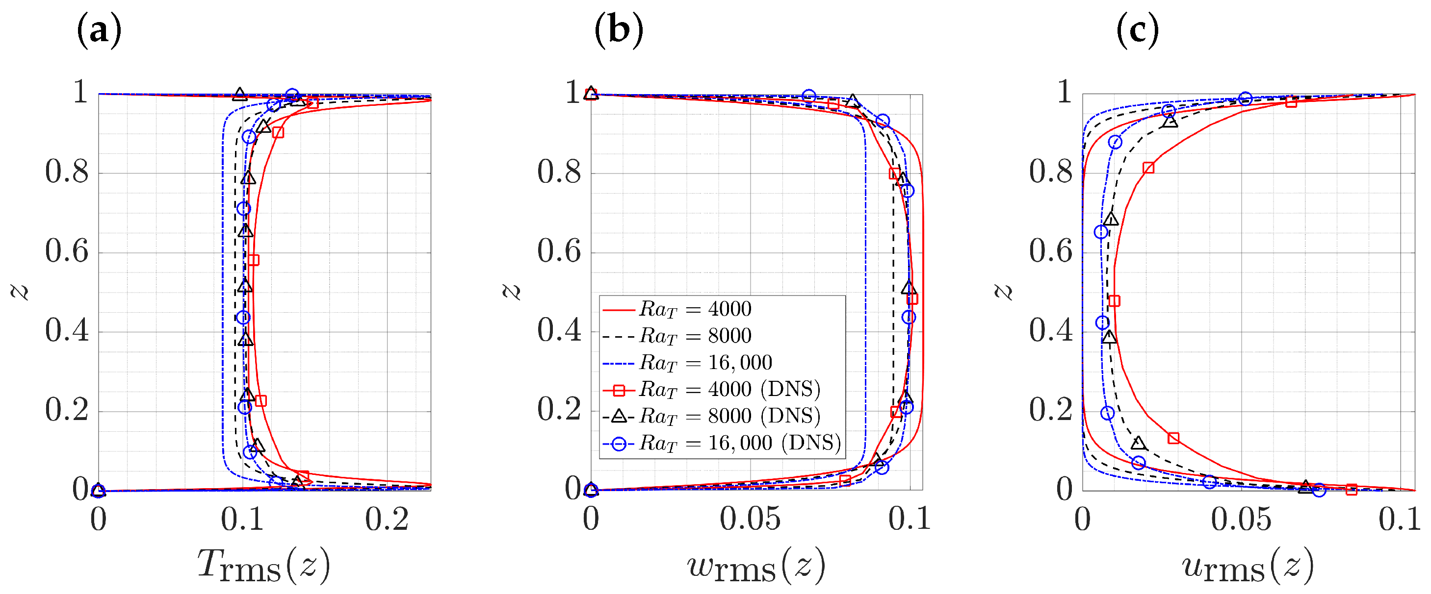
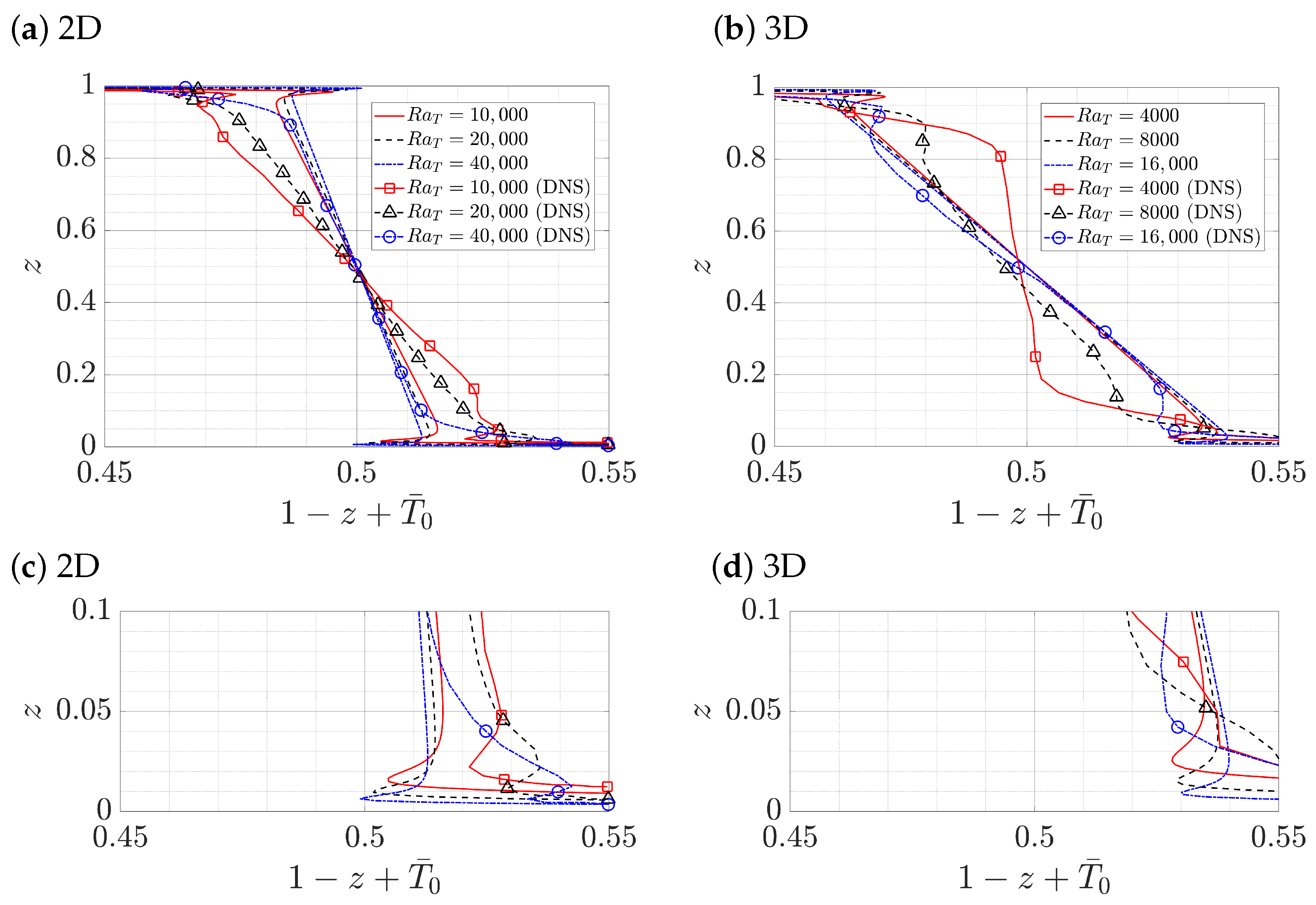
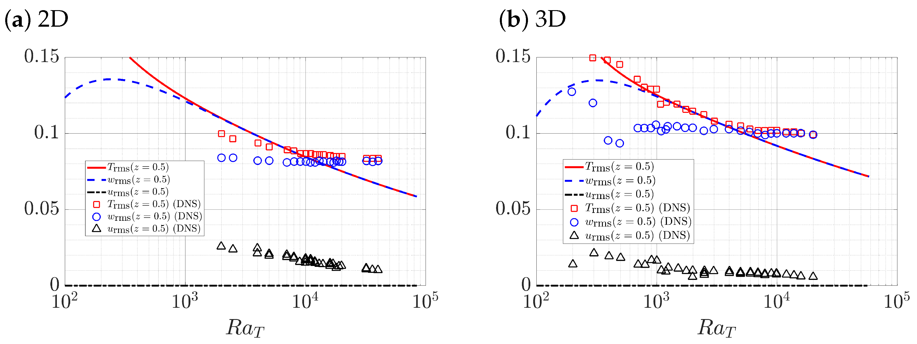
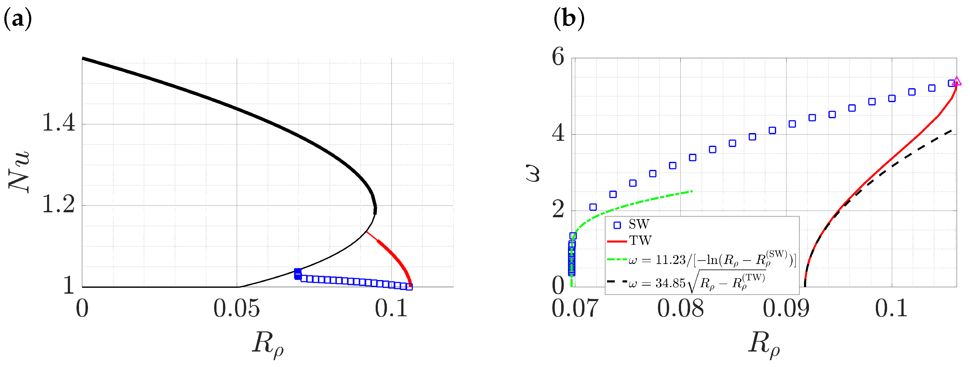
3.1. Thermal Convection with Passive Salinity $R_{\rho }=0$

In this subsection, we set $R_{\rho }=0$, indicating that the salinity is passive, in order to compare the results with thermal convection and transport of a passive scalar in a porous medium without additional contributions to the driving buoyancy term [25,26,27,28,39,52]. This subsection first compares the single-mode solutions with DNS results [25,26,27,28], as well as exact 2D steady convection rolls [26] and upper bound theory [52], all with periodic boundary conditions in the horizontal. We also compare the single-mode solutions with exact 2D steady convection rolls reached by DNS with no-flux B.C. in the horizontal [39].

Selecting a suitable wavenumber is the main difficulty of applying single-mode solutions [1,4]. Here, we choose $k_y=0$ to model a 2D flow and the wavenumber scaling $k_x=0.48R{a}_T^{0.4}$ obtained from the Fourier spectrum at $z=0.5$ in 2D DNS (Figure 10a in [27]) and (Figure 5 in [29]). For 3D results, we select the wavenumber $k_x=k_y=0.17R{a}_T^{0.52}$ based on measurement at $z=0.5$ in 3D DNS (Figure 10a in [27]). These scaling laws represent the best-fit power laws over the range of $R{a}_T$ accessible to DNS.

We first compare the harmonic components of single-mode solutions resembling steady convection rolls with the RMS temperature and velocity from DNS. We compute the RMS value over the horizontal direction from steady single-mode convection rolls using

$$\begin{array}{c}\hfill T_{\mathrm{rms}}\left(z\right)=\sqrt{2}|\widehat{T}\left(z\right)|,w_{\mathrm{rms}}\left(z\right)=\sqrt{2}|\widehat{w}\left(z\right)|/R{a}_T,u_{\mathrm{rms}}\left(z\right)=\sqrt{2}\left|\widehat{u}\left(z\right)\right|/R{a}_T,\end{array}$$

(12)

consistent with the corresponding DNS results [25,27], where the buoyancy velocity scale is employed to normalize velocities. Figure 1 shows that the RMS distribution over the vertical direction z of the single-mode solutions reproduces the qualitative behavior of the RMS values from 3D DNS (Figure 8b in [27]). For example, the temperature RMS values from both the single-mode solutions and the DNS results exhibit a peak near the top and bottom boundaries, and the location of this peak is closer to the boundary at a higher Rayleigh number. The RMS values of both temperature and vertical velocity show a nearly uniform profile in the interior ($z=0.5$) for both single-mode solutions and DNS results. For the RMS value of the horizontal velocity, the single-mode solutions also reproduce the peak values at the top and bottom boundaries as observed in the DNS. However, the single-mode solutions always predict a zero horizontal velocity RMS in the interior similar to the heat-exchanger model [25,27], although the DNS results indicate a non-zero value.

Figure 2 then compares the mean temperature $1-z+{\overline{T}}_0$ obtained from single-mode solutions with DNS results in both 2D (Figure 3a in [25]) and 3D (Figure 7 in [27]) at the corresponding Rayleigh number. Here, we observe that the single-mode solutions accurately reproduce the mean temperature gradient in the interior from DNS, in particular at high Rayleigh numbers. The heat-exchanger model which is an exact solution for unbounded convection in a porous medium was shown to describe well the mean temperature gradient in the interior; see 2D (Equations (3) and (4) in [25]) and 3D (Equation (3.2) in [27]). Considering the single-mode solutions satisfying (7) and making the reasonable assumption ${\partial }_z^2\widehat{w}(z=0.5)=0$ (cf. Figure 1), we notice that the single-mode solutions reduce to

$$\begin{array}{c}\hfill -1+{\partial }_z{\overline{T}}_0(z=0.5)=-\frac{k_x^2+k_y^2}{Ra}.\end{array}$$

(13)

The mean temperature gradient in (13) is the same as that within the heat-exchanger model [25,27]. Here, the single-mode solutions also reproduce the trend observed in DNS data [25,27] that the mean temperature gradient is closer to zero (isothermal interiors) at a larger Rayleigh number in 2D results (Figure 2a), but farther from zero in 3D results (Figure 2b), observations based on the assumed wavenumber scaling $k_x\sim R{a}_T^{0.4}$ in 2D [25] and $k_x=k_y\sim R{a}_T^{0.52}$ in 3D [27]. This wavenumber-Rayleigh-number scaling explains, in conjunction with (13), the different Rayleigh number trends of the interior mean temperature gradient observed in 2D and 3D using single-mode solutions.

The comparisons presented in Figure 2 also show that the single-mode solutions reproduce the mean temperature overshoot, a thin stably stratified layer near both boundaries. This overshoot appears closer to the boundary at higher Rayleigh numbers, a fact evident in both the single-mode solutions and DNS results; see the zoom near the bottom boundary in Figure 2c,d. Although the precise values of the overshoot temperature in the single-mode solutions are not fully accurate, this observation nonetheless suggests that the single-mode solutions preserve certain physical mechanisms responsible for this overshot, which is also present in single-mode solutions for RBC [1,2,3]. In the high Rayleigh number and high wavenumber asymptotic regime of porous media convection, an overshoot near the boundary is also found (Figure 3 in [14]), but is absent in the same asymptotic regime in RBC [13]. Such mixed convective-stably-stratified fluids are extensively studied in penetrative convection (Section 7.3.4 in [63]) using both numerical simulations [64,65,66,67] and experiments [67,68,69,70,71]; see the recent review [72].

In Figure 3, we compare the Rayleigh number trend of the RMS values in the interior, at $z=0.5$, obtained from single-mode solutions with DNS results in both 2D (Figure 3b in [25]) and 3D (Figure 8a in [27]). Evidently, the single-mode theory substantially underestimates $T_{\mathrm{rms}}(z=0.5)$ and $w_{\mathrm{rms}}(z=0.5)$ at large $R{a}_T$, which appear to saturate with increasing $R{a}_T$ in DNS results, but continue to decrease within single-mode theory, although the latter reproduces the DNS observation that these quantities approach one another at high $R{a}_T$. In fact, the single-mode quantities overlap at large $R{a}_T$, a direct consequence of (7a) and the assumption that ${\partial }_z^2\widehat{w}(z=0.5)=0$ at high $R{a}_T$, together with (12). However, this relation breaks down at low Rayleigh numbers as shown in both DNS and single-mode solutions. We also examined the profiles of the single-mode solutions at a low Rayleigh number (not shown here), and found that $\widehat{w}$ is no longer uniform in the interior, leading directly to the observed difference between $T_{\mathrm{rms}}(z=0.5)$ and $w_{\mathrm{rms}}(z=0.5)$. For high Rayleigh numbers, the DNS results indicate that both $T_{\mathrm{rms}}(z=0.5)$ and $w_{\mathrm{rms}}(z=0.5)$ tend to a constant value, which is not observed in the single-mode solutions. Moreover, in single-mode theory $u_{\mathrm{rms}}(z=0.5)$ remains zero at the Rayleigh numbers reported here, while the DNS data show a non-zero value with a slow decrease to zero as $R{a}_T$ increases.

We next analyze the heat transport by computing the Nusselt number

$$\begin{array}{c}\hfill Nu:=1-{\langle {\partial }_z{\overline{T}}_0(z=0,t)\rangle }_t.\end{array}$$

(14)

where ${\langle ·\rangle }_t$ is the average over time. Figure 4a shows $Nu$ as a function of $R{a}_T$ obtained from single-mode solutions with the 2D $k_x=0.48R{a}_T^{0.4}$ wavenumber scaling compared with 2D DNS data (Figure 2 in [25] and Figure 5b in [26]), exact 2D steady convection rolls (Figure 5b in [26]), and upper bound theory (Figure 5 in [52]). Figure 4b shows the corresponding results with the 3D $k_x=k_y=0.17R{a}_T^{0.52}$ wavenumber scaling compared with DNS data (Figure 2a in [27] and Table 1 in [28]) and upper bound theory (Figure 5 in [52]). Near onset, $R{a}_T\le 100$, the single-mode solutions deviate from the DNS results because the employed wavenumber scaling based on high $R{a}_T$ DNS data may not apply in this regime. Compared with DNS data [25,26,27], the single-mode solutions overpredict $Nu$ in the small Rayleigh number regime $R{a}_T\in [100,1000]$, but underestimate it in the high $R{a}_T$ regime. We also fit $Nu$ over $R{a}_T$ for $R{a}_T\in [{10}^3,8.4\times {10}^4]$ to obtain $Nu\approx 0.154R{a}_T^{0.666}$ for single-mode solutions with the 2D wavenumber scaling. For the 3D results, the $Nu$ scaling is $Nu\approx 0.108R{a}_T^{0.723}$ for $R{a}_T\in [{10}^3,5.8\times {10}^4]$. Here, we note that the scaling exponent $\eta$ of $Nu\sim R{a}_T^{\eta }$ is lower than that observed in DNS suggesting $Nu\sim R{a}_T$ at high $R{a}_T$ [25,26,27,28]. Such an inconsistent $Nu$ scaling may result from the underlying single-mode assumption precluding the presence of proto-plumes that emerge near the boundary [25,27] but display a different wavenumber scaling from that employed here (Figure 10 in [27]). The steady-state assumption may also lead to a difference in $Nu$ from DNS results: the exact 2D steady convection rolls involving higher order harmonics computed by Newton–Kantorovich iteration exhibit a scaling law $Nu\sim R{a}_T^{0.6}$ [26] that differs from the $Nu\sim R{a}_T$ scaling observed in DNS [25,26,27,28,52]. Moreover, the secondary Hopf bifurcation of exact 2D steady convection rolls present in DNS leads to secondary boundary modes [26,73,74,75], but such a secondary bifurcation is absent from the single-mode formulation. However, the $Nu$ scaling obtained from the single-mode solutions remains lower than the upper bound from upper bound theory [52], as shown in Figure 4.

The $Nu$ scaling obtained from single-mode solutions also depends on the assumed wavenumber, and the single-mode solutions of RBC suggest a suitable wavenumber resulting in $Nu$ close to experimental measurement [5]. Here, we further investigate the wavenumber influence on $Nu$ to identify the parameter regime in which the single-mode solutions provide a valid description of the system, focusing on 2D results ($k_y=0$). Figure 5 shows $Nu$ for a range of $k_x$ and $R{a}_T$. These values are then compared with the $Nu$ of exact 2D steady convection rolls reached in DNS (Figure 6 and Table 3 in [39]), where the domain size of the enclosure is varied. Note that the enclosure is associated with no-flux horizontal boundary conditions, and thus the associated wavenumber is computed as $k_x=n\pi /L_{x,\mathrm{NBC}}$. In the high wavenumber regime corresponding to a narrow convection cell, the single-mode solutions predict $Nu$ close to the DNS results, but the prediction begins to deviate for larger horizontal domain sizes (smaller $k_x$). This deviation can be traced to the interaction between different horizontal harmonics present in larger domains that lead to non-sinusoidal solution profiles in the horizontal (Figure 5 in [39]). A similar result is found in salt-finger convection when the corresponding single-mode solutions are compared against DNS results (Figures 2, 6 and 11 in [12]). At lower $R{a}_T$, closer to the onset, the agreement between the single-mode solutions and DNS improves; see Figure 5b, as also found in salt-finger convection (Figure 18 in [12]).

Figure 6 shows isocontours of the streamfunction $\psi$, the total temperature $1-z+T$ and the total salinity $1-z+S$. Here, the streamfunction for a two-dimensional flow is constructed as

$$\begin{array}{cc}\hfill \psi (x,z,t)=& \widehat{\psi }(z,t)e^{\mathrm{i}{k}_{x}x}+c.c.\mathrm{with}\hfill \end{array}$$

(15a)

$$\begin{array}{cc}\hfill \widehat{\psi }=& \widehat{w}/\left(\mathrm{i}{k}_x\right).\hfill \end{array}$$

(15b)

The total temperature and total salinity are both constructed from the single-mode ansatz in (5) and adding the background linear profile as in Equation (1). Figure 6 reproduces the qualitative behavior in the parameter regime of Figure 5 in [39] despite its sinusoidal structure in the horizontal. In fact, the nonsinusoidal nature of the streamfunction of the exact 2D steady convection rolls reached in DNS accounts for the $Nu$ difference between the single-mode equations and DNS shown in Figure 5. The total salinity at the higher Lewis number $Le=20$ shown in Figure 6d displays a relatively well-mixed interior compared with the corresponding result at $Le=4$ in Figure 6c, as also found in DNS observations (Figure 5 in [39]).

We now turn to the properties of the Sherwood number quantifying salinity transport and defined as

$$\begin{array}{c}\hfill Sh:=1-{\langle {\partial }_z{\overline{S}}_0(z=0,t)\rangle }_t.\end{array}$$

(16)

Figure 7 shows $Sh$ as a function of $Le$ for passive salinity ($R_{\rho }=0$) for a range of $R{a}_T$, compared with the DNS results (Figure 6 and Table 3 in [39]), on the assumption that $k_x=\pi$, $1.25\pi$, $2\pi$, $3\pi$ and $5.83\pi$ for $R{a}_T=50$, 100, 200, 400 and 1000, respectively, based on the expression $k_x=n\pi /L_{x,\mathrm{NBC}}$ with n and $L_{x,\mathrm{NBC}}$ obtained from [39]. Here, the single-mode solutions predict $Sh$ that overlaps with the DNS results at $R{a}_T=50$ over a wide range of $Le$. For high $R{a}_T$ and $Le\gtrsim 1$ the single-mode equations over-predict $Sh$ in comparison with the DNS. The single-mode solutions show a scaling law $Sh\sim L{e}^{\eta }$ with $\eta =0.52$ for $R{a}_T=50$ and $\eta =0.51$ for $R{a}_T=100$, 200, 400 and 1000 fitted within $Le\in [10,100]$. This scaling law is close to the scaling law $Sh\sim L{e}^{0.5}$ observed in DNS results [39].

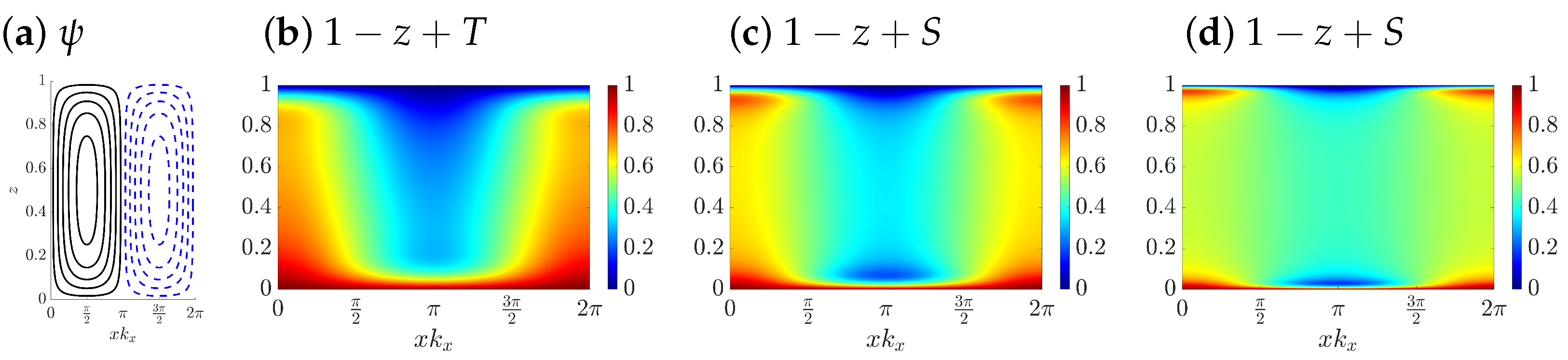
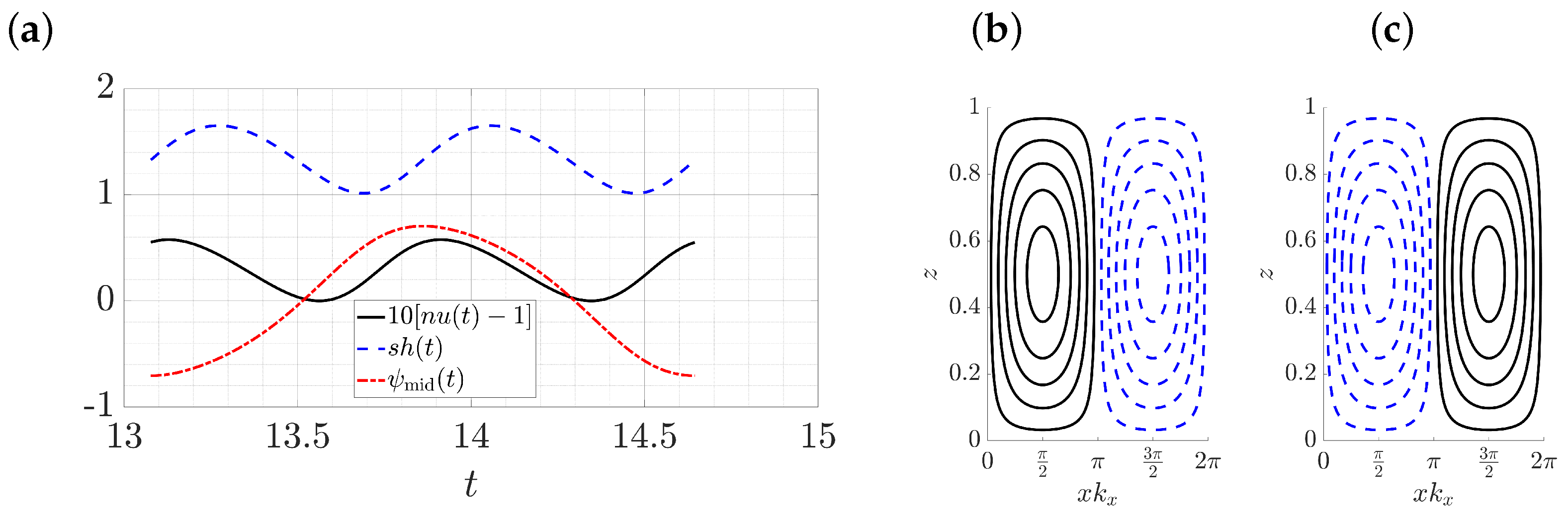
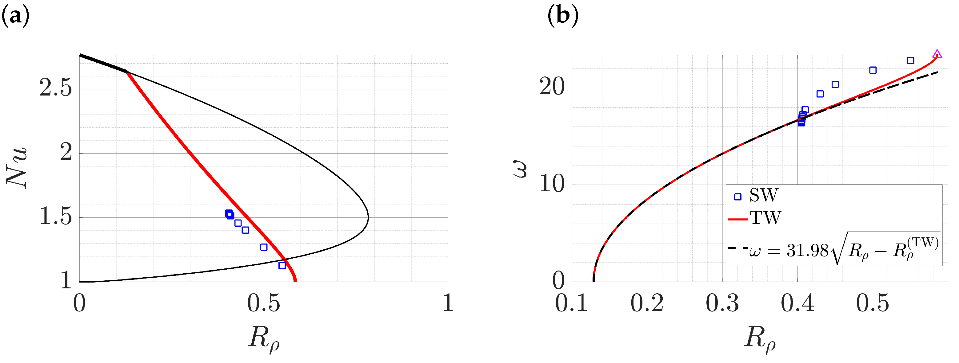
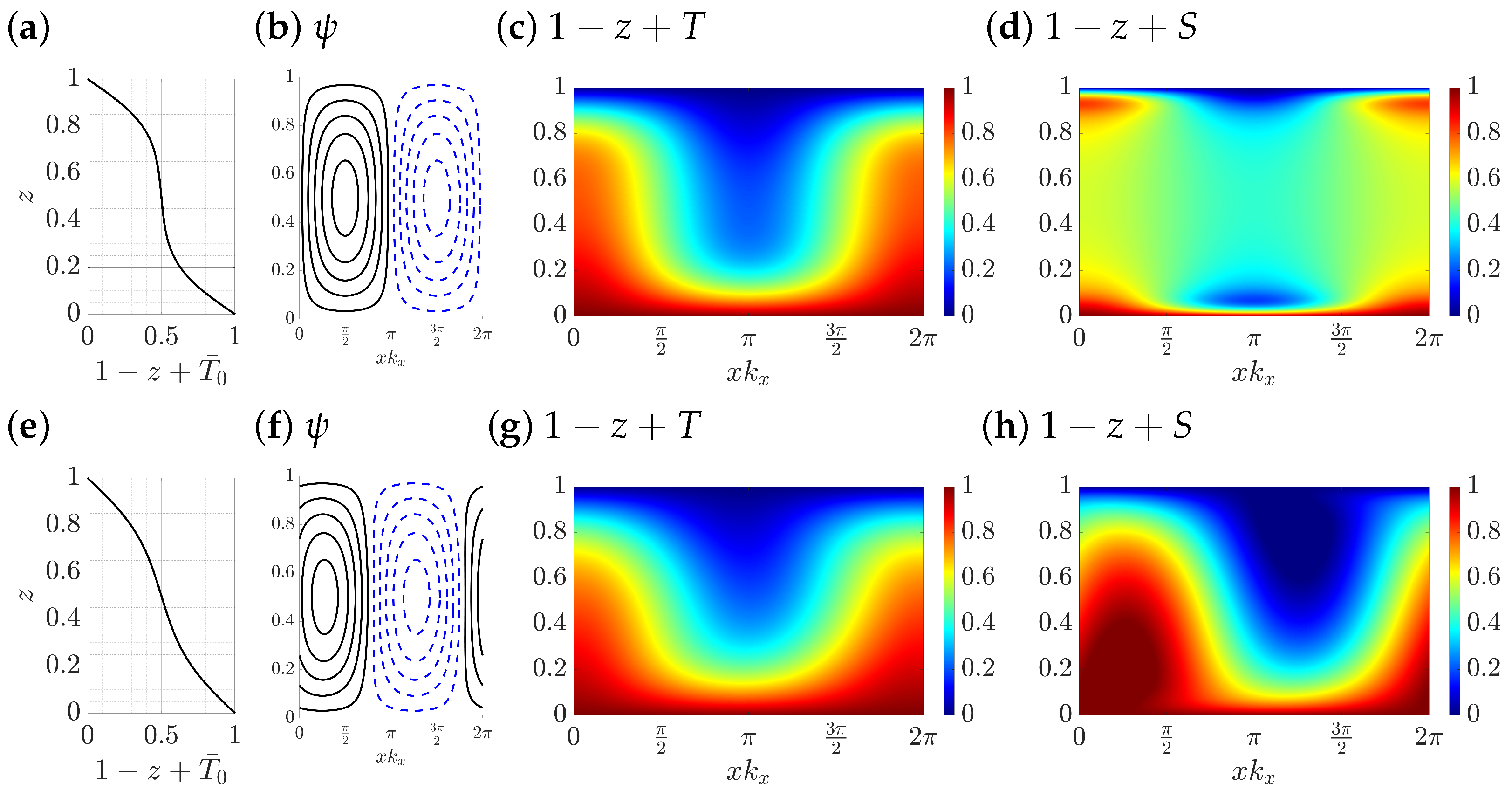
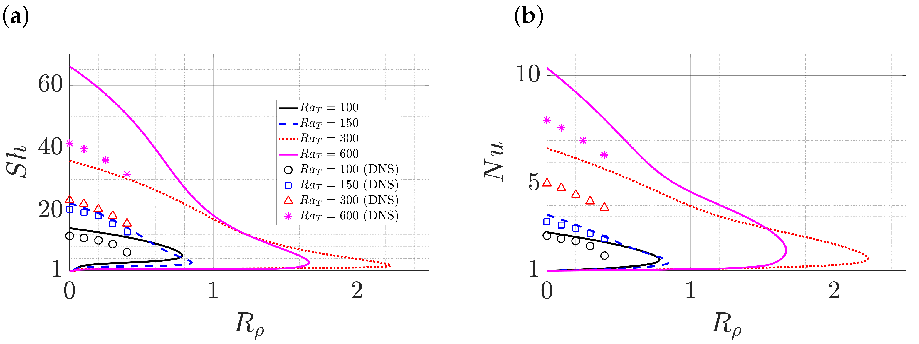
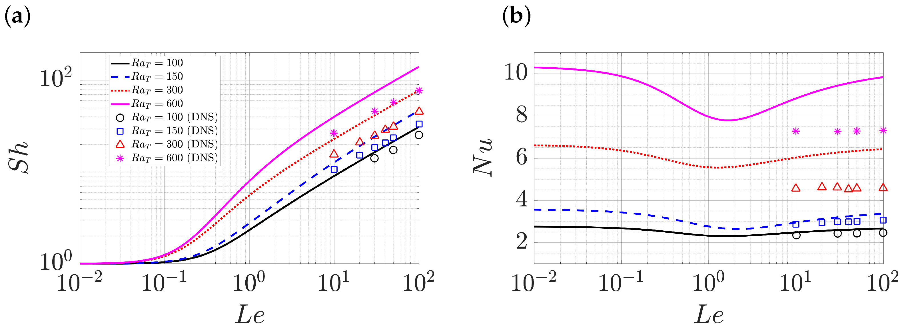
3.2. Double-Diffusive Convection with $R_{\rho }\ne 0$

In this subsection, we investigate the effect of an active salinity that also contributes to the buoyancy ($R_{\rho }\ne 0$). Here, $R_{\rho }>1$ corresponds to an overall stably stratified (bottom-heavy) configuration. The resulting configuration differs substantially from the passive case $R_{\rho }=0$ in that it admits oscillations about the conduction state. This overstable case manifests itself in the presence of a Hopf bifurcation that precedes the steady onset studied in the preceding section. In this subsection we compare the resulting standing waves, traveling waves and steady convection rolls computed from the single-mode equations with the corresponding 2D DNS results using both no-flux and periodic B.C. in the horizontal [40,43].

Figure 8a shows a standing wave (SW) over one oscillation period obtained from a simulation of the single-mode equations with real $[\widehat{w},\widehat{T},\widehat{S}]$ in terms of the quantities

$$\begin{array}{cc}\hfill nu\left(t\right):=& 1-{\partial }_z{\overline{T}}_0(z=0,t),\hfill \end{array}$$

(17a)

$$\begin{array}{cc}\hfill sh\left(t\right):=& 1-{\partial }_z{\overline{S}}_0(z=0,t),\hfill \end{array}$$

(17b)

$$\begin{array}{cc}\hfill {\psi }_{\mathrm{mid}}\left(t\right):=& \underset{x}{\max }\psi (x,z=0.5,t),\hfill \end{array}$$

(17c)

displaying values close to the 2D DNS results with no-flux B.C. in the horizontal (Figure 5 in [43]) as compared in

Table 1. Comparison of $\underset{t}{\max }{\psi }_{\mathrm{mid}}\left(t\right)$, $\underset{t}{\max }nu\left(t\right)$, $\underset{t}{\max }sh\left(t\right)$ and the oscillation period $T_p$ of standing waves obtained from the single-mode equations and DNS (Figure 5 and p. 77 in [43]) at $R{a}_T=55$, $R_{\rho }=0.1$ and $Le=5$. The single-mode solutions are associated with $k_x=\pi$, $k_y=0$ while the DNS results [43] are computed with no-flux B.C. in a horizontal domain of size $L_{x,\mathrm{NBC}}=\pi /k_x=1$.

	$\underset{\mathit{t}}{\mathit{max}}{\mathit{\psi }}_{\mathit{mid}}\left(\mathit{t}\right)$	$\underset{\mathit{t}}{\mathit{max}}\mathit{nu}\left(\mathit{t}\right)$	$\underset{\mathit{t}}{\mathit{max}}\mathit{sh}\left(\mathit{t}\right)$	Period ${\mathit{T}}_{\mathit{p}}$
Standing waves from DNS [43]	0.670	1.052	1.594	1.535
Standing wave from single-mode	0.705	1.058	1.652	1.568

. The oscillation period from the single-mode equations is $T_p=1.568$, which is also close to the DNS observation of $T_p=1.535$ [43], p. 77. Figure 8b,c show isocontours of the streamfunction at the minima and maxima of ${\psi }_{\mathrm{mid}}\left(t\right)$, indicating a complete flow reversal between these instants, in agreement with DNS results (Figure 6 in [43]) and SW observed in related problems [47,76]; the quantities $nu\left(t\right)$ and $sh\left(t\right)$ are quadratic and so oscillate with half the oscillation period.

Figure 9a shows the bifurcation diagram for the single-mode equations at $R{a}_T=53$, $Le=5$, $k_x=2\pi /L_x=\pi$ corresponding to $L_x=2$. This parameter regime displays traveling waves (TW) in DNS with periodic B.C. in the horizontal at $R_{\rho }=0.1$ (Figure 8b in [43]). Here, the single-mode solutions also show a branch of TW (in red) and the TW branch is stable at $R_{\rho }=0.1$, consistent with DNS observation [43]. The TW branch loses stability at $R_{\rho }=0.0954$ through a secondary Hopf bifurcation prior to its termination on the lower branch of steady convection (in black). Figure 9a shows that both TW and SW bifurcate supercritically from the trivial solution, and that the TW branch displays a larger $Nu$ than the SW branch. This is consistent with the prediction that a stable branch emerges from a Hopf bifurcation with $O\left(2\right)$ symmetry whenever both TW and SW branches bifurcate supercritically and that the larger amplitude branch measured by $Nu$ is then stable [46,48,77].

Figure 9b displays the oscillation frequency $\omega =2\pi /T_p$ for both TW and SW. Both start at ${\omega }_{\mathrm{Hopf}}=5.36981$ at the Hopf bifurcation point $R_{\rho }=0.10615$ from the trivial solution, and both decrease to zero with decreasing $R_{\rho }$, at which point they terminate on the lower branch of (unstable) steady rolls. The TW terminate in a local parity-breaking bifurcation at $R_{\rho }^{\left(\mathrm{TW}\right)}=0.0918$ and do so as $\omega \sim \sqrt{R_{\rho }-R_{\rho }^{\left(\mathrm{TW}\right)}}$[49,79,80] while the SW terminate at $R_{\rho }^{\left(\mathrm{SW}\right)}=0.06966838$ in a global bifurcation and do so as $\omega \sim 1/[-ln(R_{\rho }-R_{\rho }^{\left(\mathrm{SW}\right)})]$, cf. [48,78]. The resulting bifurcation diagram resembles those found in [47,49,79].

At the slightly different Rayleigh number $R{a}_T=55$, the other parameters being the same ($Le=5$, $R_{\rho }=0.1$, $L_x=2$), DNS with periodic B.C. in the horizontal instead shows the existence of steady convection rolls (Figure 8a in [43]), while the single-mode solutions also give steady convection rolls, as shown in the top row of Figure 10. For comparison, the bottom row of Figure 10 shows the corresponding solution profiles for the TW at $R{a}_T=53$. Here, both steady convection rolls and traveling waves show streamlines resembling counter-rotating rolls, but the isocontours of the total temperature and total salinity of the traveling waves reveal profiles that are less well-mixed than in steady convection, as also found in DNS (Figure 8 in [43]). The left-right asymmetry of the TW profiles is indicative of propagation.

Table 2. Comparison of ${\psi }_{\max }$, $Nu$, $Sh$ and c between single-mode solutions and DNS for steady convection rolls at $R{a}_T=55$ and traveling waves at $R{a}_T=53$. Other parameters are $R_{\rho }=0.1$, $Le=5$, $k_x=\pi$ and $k_y=0$; the DNS results are computed with periodic B.C. in the horizontal with period $L_x=2\pi /k_x=2$ (Figure 8 and p. 79 in [43]).

	${\mathit{\psi }}_{\mathbf{max}}$	$\mathit{Nu}$	$\mathit{Sh}$	c
Steady convection rolls from DNS $(R{a}_T=55)$ [43]	1.924	1.371	3.320	0
Steady convection rolls from single-mode $(R{a}_T=55)$	1.812	1.341	3.387	0
Traveling wave from DNS $(R{a}_T=53)$ [43]	0.869	1.087	1.865	−1.03
Traveling wave from single-mode $(R{a}_T=53)$	0.848	1.083	1.828	−1.07

further reports the maximum value of streamfunction ${\psi }_{\max }:=\underset{x,z,t}{\max }\psi (x,z,t)$, $Nu$ and $Sh$ of steady convection rolls and traveling waves obtained from single-mode solutions. These values are then compared with the DNS values reported in Figure 8 in [43]. Table 2 also includes the phase speed c of traveling waves obtained from single-mode solutions for comparison with DNS results [43], p. 79. Note that $c=0$ for steady solutions by definition. The comparison in Table 2 shows that the single-mode solutions quite accurately predict the correct values of ${\psi }_{\max }$, $Nu$, $Sh$ and c for both steady convection rolls and traveling waves.

Figure 11a shows the bifurcation diagram for $R{a}_T=100$, $Le=20$, $k_x=\pi$ and $k_y=0$. Here, the stable TW branch connects to the upper branch of steady convection rolls instead of the lower branch. The connection stabilizes steady rolls for $R_{\rho }<R_{\rho }^{\left(\mathrm{TW}\right)}$. A similar bifurcation diagram with the TW branch terminating at the upper branch was computed for binary fluid convection (Figure 1 in [81]). The transition between the diagrams in Figure 9 and Figure 11 is the result of increasing $R{a}_T$ and $Le$ and occurs when the TW termination point $R_{\rho }^{\left(\mathrm{TW}\right)}$ passes through the fold on the branch of steady rolls, cf. Figure 3 in [49]. Figure 11a also shows $Nu$ for the unstable SW but these may undergo a fold at lower $R_{\rho }$ that renders them unstable even with no-flux B.C. Figure 11b displays $\omega =2\pi /T_p$ for SW and $\omega =\left|c\right|k_x$ for TW, both of which start from ${\omega }_{\mathrm{Hopf}}=23.40889$ at the Hopf bifurcation point $R_{\rho }=0.58548$ from the trivial solution and decrease with decreasing $R_{\rho }$. Near $R_{\rho }^{\left(\mathrm{TW}\right)}=0.129$, where the TW branch connects to the upper branch of steady convection rolls, the TW branch once again displays the $c\sim \sqrt{R_{\rho }-R_{\rho }^{\left(\mathrm{TW}\right)}}$ behavior consistent with theoretical analysis [49,79,80].

Figure 12 shows the solution profile at $R_{\rho }=0.4$ for both unstable steady convection rolls and stable traveling waves. Here, the mean temperature of the traveling waves is closer to a linear profile, a fact that is consistent with the lower $Nu$ of traveling waves shown in Figure 11. The isocontours of total temperature and salinity of traveling waves also show profiles that are less well-mixed in the interior than in the corresponding steady convection rolls, cf. Figure 10.

Figure 13 shows $Sh$ and $Nu$ for single-mode solutions in the form of steady convection rolls as a function of $R_{\rho }$ for $R{a}_T=100$, 150, 300 and 600 with wavenumbers $k_x=n\pi /L_{x,\mathrm{NBC}}=\pi$, $2\pi$, $2\pi$, and $4\pi$, respectively. We select these wavenumbers based on $L_{x,\mathrm{NBC}}=1$ and the number of convection cells observed in the DNS [40], p. 1266. Here, single-mode solutions also reproduce the qualitative trend observed in DNS (Figure 5 in [40]), namely that $Sh$ and $Nu$ decrease as $R_{\rho }$ increases, corresponding to a stronger stabilizing effect of the salinity gradient. In particular, the single-mode solutions predict $Nu$ and $Sh$ larger than or equal to those of steady convection rolls reached by DNS for these $R{a}_T$ values, similar to the observations in Figure 5 and Figure 7 as well as the comparison in salt-finger convection [12]. Single-mode solutions in the form of steady convection rolls also exist in the stably stratified regime $R_{\rho }>1$ as a result of diffusivity difference between temperature and salinity. The single-mode solutions fold at $R_{\rho }=1.665$ when $R{a}_T=600$, which is consistent with DNS observation showing that the final state at $R_{\rho }=3$ is the conduction state (Figure 7 in [40]).

Finally, Figure 14 fixes $R_{\rho }=0.2$ and presents $Sh$ and $Nu$ as a function of $Le$. The wavenumber $k_x$ employed for each $R{a}_T$ is selected in the same way as in Figure 13 to facilitate direct comparison with the corresponding DNS results (Figure 4 in [40]). We see that for the single-mode solutions $Sh\sim L{e}^{\eta }$ within $Le\in [10,100]$ with $\eta =0.53$, 0.56, 0.53 and 0.54 for $R{a}_T=100$, 150, 300 and 600, respectively. These scaling laws closely follow the trend $Sh\sim L{e}^{0.5}$ observed in the DNS data [40], although a slight difference exists. The influence of $Le$ on $Nu$ is also relatively smaller compared with $Sh$, as also found in DNS [40]. Moreover, the plot of $Nu$ as a function of $Le$ within the range $Le\in [{10}^{-2},{10}^2]$ shows a minimum near $Le\approx 1$ similar to the trend $\psi \sim Le$ at $R_{\rho }=0.1$ (Figure 11b in [43]). This is undoubtedly a consequence of the fact that when $Le=1$ the system ceases to be double-diffusive.

4. Conclusions and Future Work

This work employs single-mode equations to analyze both convection and double-diffusive convection in a porous medium where the Darcy law provides large-scale damping. The single-mode equations are obtained from a severely truncated Fourier expansion in the horizontal, but preserve the nonlinear interaction between horizontally averaged mode and a single harmonic mode of the convective state. The single-mode equations fully resolve the vertical direction providing strongly nonlinear solutions. Despite the shortcomings of this approach, we found the single-mode solutions reproduce much of the observed phenomenology identified in high Rayleigh number simulations.

We first considered thermal convection where salinity can be viewed as a passive scalar ($R_{\rho }=0$). In this case, convection sets via a steady state bifurcation. The resulting steady convection rolls are well captured by steady solutions of the single-mode equations, which reproduce the qualitative behavior of the RMS profiles (vertical velocity, horizontal velocity and temperature), and the mean temperature profile of the time-dependent state at high Rayleigh numbers, obtained using DNS [25,27]. The single-mode solutions are also consistent with the heat-exchanger model that describes well the mean temperature gradient in the interior [25,27]. The $Nu$ predicted by the single-mode solutions lies below the theoretical upper bound [52] and reveals a scaling law with Rayleigh number close to that followed by exact 2D steady convection rolls [26]. This prediction differs from large aspect ratio DNS results [25,26,27,28] where the presence of additional degrees of freedom apparently enhances heat transport but agrees with DNS in small horizontal domains [39] where such degrees of freedom are suppressed.

When the salinity gradient is stabilizing ($R_{\rho }\ne 0$) the situation is quite different: the system becomes overstable and the conduction state loses stability to oscillations. The resulting traveling and standing waves can still be computed within single-mode theory and both are found to bifurcate supercritically and terminate on the subcritical branch of steady rolls as predicted by theory [78,79,80]. Of the two competing states, TW and SW, the larger amplitude state as measured by the Nusselt number, is stable, also in agreement with theoretical prediction [48] and consistent with DNS observations [43]. The $Sh$ obtained from single-mode solutions shows a scaling law over $Le$ close to DNS observation for both active [40] and passive [39] salinity. The single-mode solutions are derived with the assumption of horizontal periodic boundary conditions, but also show agreement with DNS using no-flux boundary conditions in the horizontal [39,40,43] after mirroring the domain.

The results here suggest the promise of this computationally tractable single-mode approach and open up new directions for future work. For example, single-mode solutions may be further applied to other flow configurations where columnar coherent structures are dominant due to inherent or imposed large-scale damping. The single-mode equations also have the potential to be further improved by systematically including higher-order harmonics in a computationally efficient manner. For example, DNS results show a wavenumber scaling near the boundary different from that in the interior in high Rayleigh number convection [27], directly motivating a "two-mode" reduced-order model. Including higher order harmonics may also suffice to capture the secondary Hopf bifurcation of exact 2D steady convection rolls leading to wall modes [26,73,74,75], promising further improvement in the predictive power of this approach.

References

1. Herring, J.R. Investigation of problems in thermal convection. J. Atmos. Sci. 1963, 20, 325–338. [Google Scholar] [CrossRef]
2. Herring, J.R. Investigation of problems in thermal convection: Rigid boundaries. J. Atmos. Sci. 1964, 21, 277–290. [Google Scholar] [CrossRef]
3. Elder, J.W. The temporal development of a model of high Rayleigh number convection. J. Fluid Mech. 1969, 35, 417–437. [Google Scholar] [CrossRef]
4. Gough, D.O.; Spiegel, E.A.; Toomre, J. Modal equations for cellular convection. J. Fluid Mech. 1975, 68, 695–719. [Google Scholar] [CrossRef]
5. Toomre, J.; Gough, D.O.; Spiegel, E.A. Numerical solutions of single-mode convection equations. J. Fluid Mech. 1977, 79, 1–31. [Google Scholar] [CrossRef]
6. Gough, D.O.; Toomre, J. Single-mode theory of diffusive layers in thermohaline convection. J. Fluid Mech. 1982, 125, 75–97. [Google Scholar] [CrossRef]
7. Turner, J.S. The coupled turbulent transports of salt and and heat across a sharp density interface. Int. J. Heat Mass Transf. 1965, 8, 759–767. [Google Scholar] [CrossRef]
8. Crapper, P.F. Measurements across a diffusive interface. Deep Sea Res. Oceanogr. Abstr. 1975, 22, 537–545. [Google Scholar] [CrossRef]
9. Marmorino, G.O.; Caldwell, D.R. Heat and salt transport through a diffusive thermohaline interface. Deep Sea Res. Oceanogr. Abstr. 1976, 23, 59–67. [Google Scholar] [CrossRef]
10. Paparella, F.; Spiegel, E.A.; Talon, S. Shear and mixing in oscillatory doubly diffusive convection. Geophys. Astrophys. Fluid Dyn. 2002, 96, 271–289. [Google Scholar] [CrossRef]
11. Paparella, F.; Spiegel, E.A. Sheared salt fingers: Instability in a truncated system. Phys. Fluids 1999, 11, 1161–1168. [Google Scholar] [CrossRef]
12. Liu, C.; Julien, K.; Knobloch, E. Staircase solutions and stability in vertically confined salt-finger convection. J. Fluid Mech. 2022, 952, A4. [Google Scholar] [CrossRef]
13. Blennerhassett, P.J.; Bassom, A.P. Nonlinear high-wavenumber Bénard convection. IMA J. Appl. Math. 1994, 52, 51–77. [Google Scholar] [CrossRef]
14. Lewis, S.; Rees, D.A.S.; Bassom, A.P. High wavenumber convection in tall porous containers heated from below. Q. J. Mech. Appl. Math. 1997, 50, 545–563. [Google Scholar] [CrossRef]
15. Proctor, M.R.E.; Holyer, J.Y. Planform selection in salt fingers. J. Fluid Mech. 1986, 168, 241–253. [Google Scholar] [CrossRef]
16. Julien, K.; Knobloch, E. Reduced models for fluid flows with strong constraints. J. Math. Phys. 2007, 48, 065405. [Google Scholar] [CrossRef] [Green Version]
17. Taylor, G.I. Motion of solids in fluids when the flow is not irrotational. Proc. R. Soc. Lond. Ser. A 1917, 93, 99–113. [Google Scholar]
18. Proudman, J. On the motion of solids in a liquid possessing vorticity. Proc. R. Soc. Lond. Ser. A 1916, 92, 408–424. [Google Scholar]
19. Sprague, M.; Julien, K.; Knobloch, E.; Werne, J. Numerical simulation of an asymptotically reduced system for rotationally constrained convection. J. Fluid Mech. 2006, 551, 141–174. [Google Scholar] [CrossRef]
20. Grooms, I.; Julien, K.; Weiss, J.B.; Knobloch, E. Model of convective Taylor columns in rotating Rayleigh-Bénard convection. Phys. Rev. Lett. 2010, 104, 224501. [Google Scholar] [CrossRef]
21. Calkins, M.A.; Julien, K.; Tobias, S.M.; Aurnou, J.M.; Marti, P. Convection-driven kinematic dynamos at low Rossby and magnetic Prandtl numbers: Single mode solutions. Phys. Rev. E 2016, 93, 023115. [Google Scholar] [CrossRef] [PubMed] [Green Version]
22. Calkins, M.A.; Long, L.; Nieves, D.; Julien, K.; Tobias, S.M. Convection-driven kinematic dynamos at low Rossby and magnetic Prandtl numbers. Phys. Rev. Fluids 2016, 1, 083701. [Google Scholar] [CrossRef]
23. Yang, Y.; van der Poel, E.P.; Ostilla-Mónico, R.; Sun, C.; Verzicco, R.; Grossmann, S.; Lohse, D. Salinity transfer in bounded double diffusive convection. J. Fluid Mech. 2015, 768, 476–491. [Google Scholar] [CrossRef] [Green Version]
24. Xie, J.H.; Julien, K.; Knobloch, E. Jet formation in salt-finger convection: A modified Rayleigh–Bénard problem. J. Fluid Mech. 2019, 858, 228–263. [Google Scholar] [CrossRef]
25. Hewitt, D.R.; Neufeld, J.A.; Lister, J.R. Ultimate regime of high Rayleigh number convection in a porous medium. Phys. Rev. Lett. 2012, 108, 224503. [Google Scholar] [CrossRef] [Green Version]
26. Wen, B.; Corson, L.T.; Chini, G.P. Structure and stability of steady porous medium convection at large Rayleigh number. J. Fluid Mech. 2015, 772, 197–224. [Google Scholar] [CrossRef] [Green Version]
27. Hewitt, D.R.; Neufeld, J.A.; Lister, J.R. High Rayleigh number convection in a three-dimensional porous medium. J. Fluid Mech. 2014, 748, 879–895. [Google Scholar] [CrossRef] [Green Version]
28. Pirozzoli, S.; De Paoli, M.; Zonta, F.; Soldati, A. Towards the ultimate regime in Rayleigh–Darcy convection. J. Fluid Mech. 2021, 911, R4. [Google Scholar] [CrossRef]
29. Hewitt, D.R. Vigorous convection in porous media. Proc. R. Soc. A 2020, 476, 20200111. [Google Scholar] [CrossRef]
30. Nield, D.A.; Bejan, A. Convection in Porous Media; Springer: Berlin/Heidelberg, Germany, 2006. [Google Scholar]
31. Vafai, K. Handbook of Porous Media; CRC Press: Boca Raton, FL, USA, 2015. [Google Scholar]
32. Mojtabi, A.; Charrier-Mojtabi, M.C. Double-diffusive convection in porous media. In Handbook of Porous Media; CRC Press: Boca Raton, FL, USA, 2005; pp. 287–338. [Google Scholar]
33. Cheng, P. Heat transfer in geothermal systems. In Advances in Heat Transfer; Elsevier: Amsterdam, The Netherlands, 1979; Volume 14, pp. 1–105. [Google Scholar]
34. Wooding, R.A.; Tyler, S.W.; White, I. Convection in groundwater below an evaporating salt lake: 1. Onset of instability. Water Resour. Res. 1997, 33, 1199–1217. [Google Scholar] [CrossRef]
35. Wooding, R.A.; Tyler, S.W.; White, I.; Anderson, P.A. Convection in groundwater below an evaporating salt lake: 2. Evolution of fingers or plumes. Water Resour. Res. 1997, 33, 1219–1228. [Google Scholar] [CrossRef]
36. Huppert, H.E.; Neufeld, J.A. The fluid mechanics of carbon dioxide sequestration. Annu. Rev. Fluid Mech. 2014, 46, 255–272. [Google Scholar] [CrossRef]
37. Neufeld, J.A.; Hesse, M.A.; Riaz, A.; Hallworth, M.A.; Tchelepi, H.A.; Huppert, H.E. Convective dissolution of carbon dioxide in saline aquifers. Geophys. Res. Lett. 2010, 37, L22404. [Google Scholar] [CrossRef]
38. Caltagirone, J.P. Thermoconvective instabilities in a horizontal porous layer. J. Fluid Mech. 1975, 72, 269–287. [Google Scholar] [CrossRef]
39. Trevisan, O.V.; Bejan, A. Mass and heat transfer by high Rayleigh number convection in a porous medium heated from below. Int. J. Heat Mass Transf. 1987, 30, 2341–2356. [Google Scholar] [CrossRef]
40. Rosenberg, N.D.; Spera, F.J. Thermohaline convection in a porous medium heated from below. Int. J. Heat Mass Transf. 1992, 35, 1261–1273. [Google Scholar] [CrossRef]
41. Goyeau, B.; Songbe, J.P.; Gobin, D. Numerical study of double-diffusive natural convection in a porous cavity using the Darcy-Brinkman formulation. Int. J. Heat Mass Transf. 1996, 39, 1363–1378. [Google Scholar] [CrossRef]
42. Mamou, M.; Vasseur, P.; Bilgen, E. Double-diffusive convection instability in a vertical porous enclosure. J. Fluid Mech. 1998, 368, 263–289. [Google Scholar] [CrossRef]
43. Mamou, M.; Vasseur, P. Thermosolutal bifurcation phenomena in porous enclosures subject to vertical temperature and concentration gradients. J. Fluid Mech. 1999, 395, 61–87. [Google Scholar] [CrossRef]
44. Mahidjiba, A.; Mamou, M.; Vasseur, P. Onset of double-diffusive convection in a rectangular porous cavity subject to mixed boundary conditions. Int. J. Heat Mass Transf. 2000, 43, 1505–1522. [Google Scholar] [CrossRef]
45. Bahloul, A.; Boutana, N.; Vasseur, P. Double-diffusive and Soret-induced convection in a shallow horizontal porous layer. J. Fluid Mech. 2003, 491, 325–352. [Google Scholar] [CrossRef]
46. Knobloch, E.; Deane, A.E.; Toomre, J.; Moore, D.R. Doubly diffusive waves. Contemp. Math. 1986, 56, 203–216. [Google Scholar]
47. Deane, A.E.; Knobloch, E.; Toomre, J. Traveling waves and chaos in thermosolutal convection. Phys. Rev. A 1987, 36, 2862–2869. [Google Scholar] [CrossRef] [PubMed]
48. Knobloch, E. Oscillatory convection in binary mixtures. Phys. Rev. A 1986, 34, 1538–1549. [Google Scholar] [CrossRef]
49. Knobloch, E.; Moore, D.R. Minimal model of binary fluid convection. Phys. Rev. A 1990, 42, 4693–4709. [Google Scholar] [CrossRef]
50. Predtechensky, A.A.; McCormick, W.D.; Swift, J.B.; Rossberg, A.G.; Swinney, H.L. Traveling wave instability in sustained double-diffusive convection. Phys. Fluids 1994, 6, 3923–3935. [Google Scholar] [CrossRef] [Green Version]
51. Predtechensky, A.A.; McCormick, W.D.; Swift, J.B.; Noszticzius, Z.; Swinney, H.L. Onset of traveling waves in isothermal double diffusive convection. Phys. Rev. Lett. 1994, 72, 218–221. [Google Scholar] [CrossRef]
52. Otero, J.; Dontcheva, L.A.; Johnston, H.; Worthing, R.A.; Kurganov, A.; Petrova, G.; Doering, C.R. High-Rayleigh-number convection in a fluid-saturated porous layer. J. Fluid Mech. 2004, 500, 263–281. [Google Scholar] [CrossRef] [Green Version]
53. Stern, M.E. Collective instability of salt fingers. J. Fluid Mech. 1969, 35, 209–218. [Google Scholar] [CrossRef]
54. Holyer, J.Y. The stability of long, steady, two-dimensional salt fingers. J. Fluid Mech. 1984, 147, 169–185. [Google Scholar] [CrossRef]
55. Radko, T. Double-Diffusive Convection; Cambridge University Press: Cambridge, MA, USA, 2013. [Google Scholar]
56. Uecker, H.; Wetzel, D.; Rademacher, J.D.M. pde2path-A Matlab package for continuation and bifurcation in 2D elliptic systems. Numer. Math. Theory Methods Appl. 2014, 7, 58–106. [Google Scholar] [CrossRef]
57. Uecker, H. Numerical Continuation and Bifurcation in Nonlinear PDEs; Springer: Berlin/Heidelberg, Germany, 2021. [Google Scholar]
58. Weideman, J.A.; Reddy, S.C. A MATLAB differentiation matrix suite. ACM Trans. Math. Software 2000, 26, 465–519. [Google Scholar] [CrossRef] [Green Version]
59. Uecker, H. pde2path without Finite Elements. 2021. Available online: http://www.staff.uni-oldenburg.de/hannes.uecker/pde2path/tuts/modtut.pdf (accessed on 12 December 2021).
60. Burns, K.J.; Vasil, G.M.; Oishi, J.S.; Lecoanet, D.; Brown, B.P. Dedalus: A flexible framework for numerical simulations with spectral methods. Phys. Rev. Res. 2020, 2, 023068. [Google Scholar] [CrossRef]
61. Bassom, A.P.; Zhang, K. Strongly nonlinear convection cells in a rapidly rotating fluid layer. Geophys. Astrophys. Fluid Dyn. 1994, 76, 223–238. [Google Scholar] [CrossRef]
62. Rademacher, J.D.M.; Uecker, H. Symmetries, Freezing, and Hopf Bifurcations of Traveling Waves in pde2path. 2017. Available online: https://www.staff.uni-oldenburg.de/hannes.uecker/pde2path/tuts/symtut.pdf (accessed on 15 December 2021).
63. Turner, J.S. Buoyancy Effects in Fluids; Cambridge University Press: Cambridge, UK, 1979. [Google Scholar]
64. Lecoanet, D.; Le Bars, M.; Burns, K.J.; Vasil, G.M.; Brown, B.P.; Quataert, E.; Oishi, J.S. Numerical simulations of internal wave generation by convection in water. Phys. Rev. E 2015, 91, 063016. [Google Scholar] [CrossRef] [Green Version]
65. Lecoanet, D.; Quataert, E. Internal gravity wave excitation by turbulent convection. Mon. Not. R. Astron. Soc. 2013, 430, 2363–2376. [Google Scholar] [CrossRef] [Green Version]
66. Lecoanet, D.; Schwab, J.; Quataert, E.; Bildsten, L.; Timmes, F.X.; Burns, K.J.; Vasil, G.M.; Oishi, J.S.; Brown, B.P. Turbulent chemical diffusion in convectively bounded carbon flames. Astrophys. J. 2016, 832, 71. [Google Scholar] [CrossRef]
67. Couston, L.A.; Lecoanet, D.; Favier, B.; Le Bars, M. Dynamics of mixed convective–stably-stratified fluids. Phys. Rev. Fluids 2017, 2, 094804. [Google Scholar] [CrossRef]
68. Le Bars, M.; Lecoanet, D.; Perrard, S.; Ribeiro, A.; Rodet, L.; Aurnou, J.M.; Le Gal, P. Experimental study of internal wave generation by convection in water. Fluid Dyn. Res. 2015, 47, 045502. [Google Scholar] [CrossRef] [Green Version]
69. Couston, L.A.; Lecoanet, D.; Favier, B.; Le Bars, M. The energy flux spectrum of internal waves generated by turbulent convection. J. Fluid Mech. 2018, 854, R3. [Google Scholar] [CrossRef] [Green Version]
70. Bouffard, M.; Favier, B.; Lecoanet, D.; Le Bars, M. Internal gravity waves in a stratified layer atop a convecting liquid core in a non-rotating spherical shell. Geophys. J. Int. 2022, 228, 337–354. [Google Scholar] [CrossRef]
71. Léard, P.; Favier, B.; Le Gal, P.; Le Bars, M. Coupled convection and internal gravity waves excited in water around its density maximum at 4° C. Phys. Rev. Fluids 2020, 5, 024801. [Google Scholar] [CrossRef]
72. Le Bars, M.; Couston, L.A.; Favier, B.; Léard, P.; Lecoanet, D.; Le Gal, P. Fluid dynamics of a mixed convective/stably stratified system—A review of some recent works. Comptes Rendus. Phys. 2020, 21, 151–164. [Google Scholar] [CrossRef]
73. Aidun, C.K.; Steen, P.H. Transition to oscillatory convective heat transfer in a fluid-saturated porous medium. J. Thermophys. Heat Transf. 1987, 1, 268–273. [Google Scholar] [CrossRef]
74. Graham, M.D.; Steen, P.H. Plume formation and resonant bifurcations in porous-media convection. J. Fluid Mech. 1994, 272, 67–90. [Google Scholar] [CrossRef]
75. Graham, M.D.; Steen, P.H. Strongly interacting travelling waves and quasiperiodic dynamics in porous medium convection. Phys. D 1992, 54, 331–350. [Google Scholar] [CrossRef]
76. Julien, K.; Knobloch, E. Fully nonlinear oscillatory convection in a rotating layer. Phys. Fluids 1997, 9, 1906–1913. [Google Scholar] [CrossRef] [Green Version]
77. Knobloch, E.; Silber, M. Travelling wave convection in a rotating layer. Geophys. Astrophys. Fluid Dyn. 1990, 51, 195–209. [Google Scholar] [CrossRef]
78. Knobloch, E.; Proctor, M.R.E. Nonlinear periodic convection in double-diffusive systems. J. Fluid Mech. 1981, 108, 291–316. [Google Scholar] [CrossRef]
79. Dangelmayr, G.; Knobloch, E. The Takens-Bogdanov bifurcation with O(2)-symmetry. Philos. Trans. R. Soc. Lond. Ser. A 1987, 322, 243–279. [Google Scholar]
80. Greene, J.M.; Kim, J.S. The steady states of the Kuramoto-Sivashinsky equation. Phys. D 1988, 33, 99–120. [Google Scholar] [CrossRef]
81. Batiste, O.; Knobloch, E.; Alonso, A.; Mercader, I. Spatially localized binary-fluid convection. J. Fluid Mech. 2006, 560, 149–158. [Google Scholar] [CrossRef]
Figure 1. RMS profiles of (a) T rms ( z ) , (b) w rms ( z ) and (c) u rms ( z ) at R a T = 4000 , 8000, 16,000 associated with the 3D wavenumber k x = k y = 0.17 R a T 0.52 obtained from single-mode solutions (lines) compared with DNS results (Figure 8b in [27]) (lines with markers). Legend for all three panels is provided in panel (b).
Fluids 07 00373 g001
Figure 2. Comparisons of the mean temperature profiles obtained from single-mode solutions (lines) with DNS (lines with markers). Panel (a) displays 2D results at R a T = 10 , 000 , 20,000 and 40,000 using k x = 0.48 R a T 0.4 and k y = 0 compared with 2D DNS (Figure 3a in [25]). Panel (b) shows 3D results at R a T = 4000 , 8000 and 16,000 using k x = k y = 0.17 R a T 0.52 compared with 3D DNS (Figure 7 in [27]). Panels (c) and (d) show zooms of panels (a) and (b) near the bottom boundary, respectively.
Fluids 07 00373 g002
Figure 3. Comparisons of the RMS values at z = 0.5 obtained from single-mode solutions (lines) with DNS (markers). Panel (a) shows 2D results with DNS data obtained from Figure 3b in [25], while panel (b) displays 3D results with DNS data obtained from Figure 8a in [27].
Fluids 07 00373 g003
Figure 4. N u as a function of R a T from single-mode solutions (black lines). Panel (a) shows 2D results with k x = 0.48 R a T 0.4 , k y = 0 compared with DNS data (Figure 2 in [25] and Figure 5b in [26]), exact 2D steady convection rolls (Figure 5b in [26]), and upper bound theory (Figure 5 in [52]). Panel (b) displays 3D results with k x = k y = 0.17 R a T 0.52 compared with DNS data (Figure 2a in [27] and Table 1 [28]) as well as upper bound theory (Figure 5 in [52]). The single-mode solutions are stable within this severe truncation.
Fluids 07 00373 g004
Figure 5. N u as a function of the horizontal wavenumber k x for R a T = 50 , 100, 200, 400, 1000 and 2000 (from bottom to top) obtained from single-mode solutions (lines) and compared with DNS results (black squares) with k x = n π / L x , NBC using n and L x , NBC appropriate to no-flux horizontal B.C. (Figure 4 and Table 2 in [39]). Panel (b) is a zoom of panel (a).
Fluids 07 00373 g005
Figure 6. Solution profile of single-mode solutions displaying isocontours of (a) streamfunction ψ , (b) total temperature 1 z + T and (c) total salinity 1 z + S at R a T = 200 , k x = 1.89 π , and L e = 4 . Panel (d) shows the isocontours of total salinity 1 z + S at L e = 20 with other parameters unchanged. This figure is to be compared with the corresponding DNS results (Figure 5 in [39]).
Fluids 07 00373 g006
Figure 7. S h as a function of L e from single-mode solutions (lines) with R ρ = 0 compared with DNS (markers) from Figure 6 and Table 3 in [39]. The horizontal wavenumbers are chosen as k x = π , 1.25 π , 2 π , 3 π , 5.83 π for R a T = 50 , 100, 200, 400, 1000 based on k x = n π / L x , NBC with n and L x , NBC as in [39].
Fluids 07 00373 g007
Figure 8. (a) One period of a standing wave computed from the single-mode equations at R a T = 55 , R ρ = 0.1 , L e = 5 , k x = π and k y = 0 displaying 10 [ n u ( t ) 1 ] , s h ( t ) and ψ mid ( t ) as a function of t [ 13.077 , 14.645 ] with oscillation period T p = 1.568 . Panels (b) and (c) show the isocontours of the streamfunction at t = 13.077 and t = 13.861 , respectively. This figure is to be compared with the corresponding DNS results (Figures 5 and 6 in [43]).
Fluids 07 00373 g008
Figure 9. (a) Bifurcation diagram of single-mode solutions at R a T = 53 , L e = 5 , k x = π and k y = 0 , showing steady convection rolls (—), SW () and TW (). Thick lines indicate stable solutions and thin lines represent unstable solutions. (b) The temporal frequency ω = 2 π / T p of SW () and TW (), the latter computed from ω = | c | k x . The Hopf frequency is ω Hopf = 5.36981 at the Hopf bifurcation point R ρ = 0.10615 (Δ) from the trivial solution. Near the termination of the SW branch, the frequency ω decreases to zero at R ρ ( SW ) as ω 1 / [ ln ( R ρ R ρ ( SW ) ) ] (−·−) as predicted theoretically [78]. Near the termination of the TW branch, the phase velocity c of the waves decreases to zero at R ρ ( TW ) as c R ρ R ρ ( TW ) (− −) as also predicted theoretically [79,80].
Fluids 07 00373 g009
Figure 10. Top: solution profiles for steady convection rolls from the single-mode equations at R a T = 55 with isocontours of (a) streamfunction ψ , (b) total temperature 1 z + T and (c) total salinity 1 z + S . Bottom: solution profiles for a left traveling wave with c = 1.07 in the comoving frame from the single-mode equations at R a T = 53 with isocontours of (d) streamfunction ψ , (e) total temperature 1 z + T and (f) total salinity 1 z + S . Other parameters are R ρ = 0.1 , L e = 5 , k x = π and k y = 0 as used in 2D DNS with periodic B.C. in the horizontal and period L x = 2 π / k x = 2 (Figure 8 in [43]).
Fluids 07 00373 g010
Figure 11. (a) Bifurcation diagram of single-mode solutions at R a T = 100 , L e = 20 , k x = π and k y = 0 showing steady convection rolls (—) of SW () and TW (). Thick lines indicate stable solutions and thin lines represent unstable solutions. (b) The temporal frequency ω = 2 π / T p of SW () and TW (), the latter computed from ω = | c | k x . The Hopf frequency is ω Hopf = 23.40889 at the Hopf bifurcation point R ρ = 0.58548 (Δ) from the trivial solution. Near the termination of the TW branch the phase velocity c of the waves decreases to zero at R ρ ( TW ) as c R ρ R ρ ( TW ) (− −) as predicted theoretically [79,80].
Fluids 07 00373 g011
Figure 12. Top: unstable steady convection rolls from single-mode equations showing (a) mean temperature 1 z + T ¯ 0 and isocontours of (b) streamfunction ψ , (c) total temperature 1 z + T and (d) total salinity 1 z + S . Bottom: stable left traveling wave convection in the comoving frame with phase speed c = 5.31 from single-mode equations showing (e) mean temperature 1 z + T ¯ 0 and isocontours of (f) streamfunction ψ , (g) total temperature 1 z + T and (h) total salinity 1 z + S . The parameters are R a T = 100 , R ρ = 0.4 , L e = 20 , k x = π and k y = 0 .
Fluids 07 00373 g012
Figure 13. (a) S h and (b) N u , both as a function of R ρ from the single-mode equations (lines) at L e = 20 , k y = 0 and R a T = 100 , 150, 300 and 600 with wavenumbers k x = n π / L x , NBC = π , 2 π , 2 π , 4 π , respectively, compared with the corresponding DNS results (markers) (Figure 5 in [40]).
Fluids 07 00373 g013
Figure 14. (a) S h and (b) N u , both as a function of L e , from the single-mode equations (lines) at R ρ = 0.2 , k y = 0 , and R a T = 100 , 150, 300 and 600 and wavenumbers k x = n π / L x , NBC = π , 2 π , 2 π , 4 π , respectively, compared with the corresponding DNS results (markers) (Figure 4 in [40]).
Fluids 07 00373 g014