All the computational results are obtained in MATLAB
® version R2017a on a virtual machine equipped with two Intel
® Xeon
® E7-8890 v4 Processors with twenty-four cores per processor and 64GB of RAM. MATLAB’s Parallel Computing Toolbox is used to parallelize the computations. Default parameters are given in
Table 1 and do not vary throughout the numerical experiments. Using a different set of values will only affect the evaluation of the objective function and does not affect how the optimization methods described in
Section 2.4 will be implemented. The design parameters are chosen to be the phase shifts and
coordinates of the bases of the helices, and we aim to determine their optimal values that achieve maximal pumping using the methods in
Section 2.4. We consider carpets made up of a single helix (
Section 3.1), a pair of helices (
Section 3.2), and multiple helices (
Section 3.3).
Applying the hybrid method described in
Section 2.4.3 to the optimization problem (
11) entails evaluating the objective function
and its surrogate
repeatedly at different
’s. As shown in
Table 1, the spatial and temporal discretization used in
s is about ten times as coarse as the discretization used in
f. For flow meters of various sizes and carpets consisting of various numbers of helices, we compare the runtimes required to evaluate
and
. Specifically, we consider three values of the width
W of the flow meter (
7):
, 5, and 10 as well as cases of one, two, and four helices. The runtimes entailed by evaluating
and
for each combination of
W and number of helices are listed in
Table 2. Here, and for the rest of the paper, runtimes are measured in seconds by MATLAB’s
tic and
toc commands. Recall that a double integral must be evaluated to calculate
or
(see (
9)). We use MATLAB’s function
integrate2 with its default setting to approximate this integral numerically.
3.1. A Single Helix
We first consider the case of a single helix by investigating the following question: Where should the helix be placed to maximize pumping? We fix all design parameters of the helix except for the
coordinates of its base point, that is,
in the optimization problem (
11).
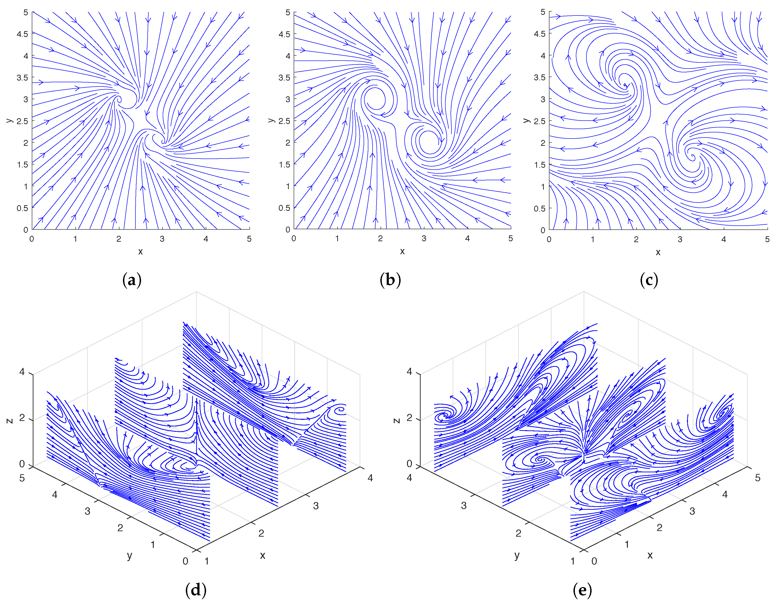
In
Figure 2, we show the streamlines drawn based on the instantaneous fluid velocity around a rotating helix. As can be seen in
Figure 2d,e, the helix moves the fluid near its tip upward while rotating, and there are also regions of downward flow away from the helix. A more detailed experimental analysis of the flow field around a single rotating helix can be found in [
31] and a numerical study was performed in [
12,
13].
Since we consider an incompressible Newtonian fluid, as the width
W of the flow meter (
7) approaches infinity, the volume of the fluid pumped through the meter goes to zero regardless of the values of the design parameters. However, in applications, only flow meters of finite sizes are of interest, and the volume of fluid that is transported through a finite flow meter does change depending on the placement of the helix relative to the flow meter.
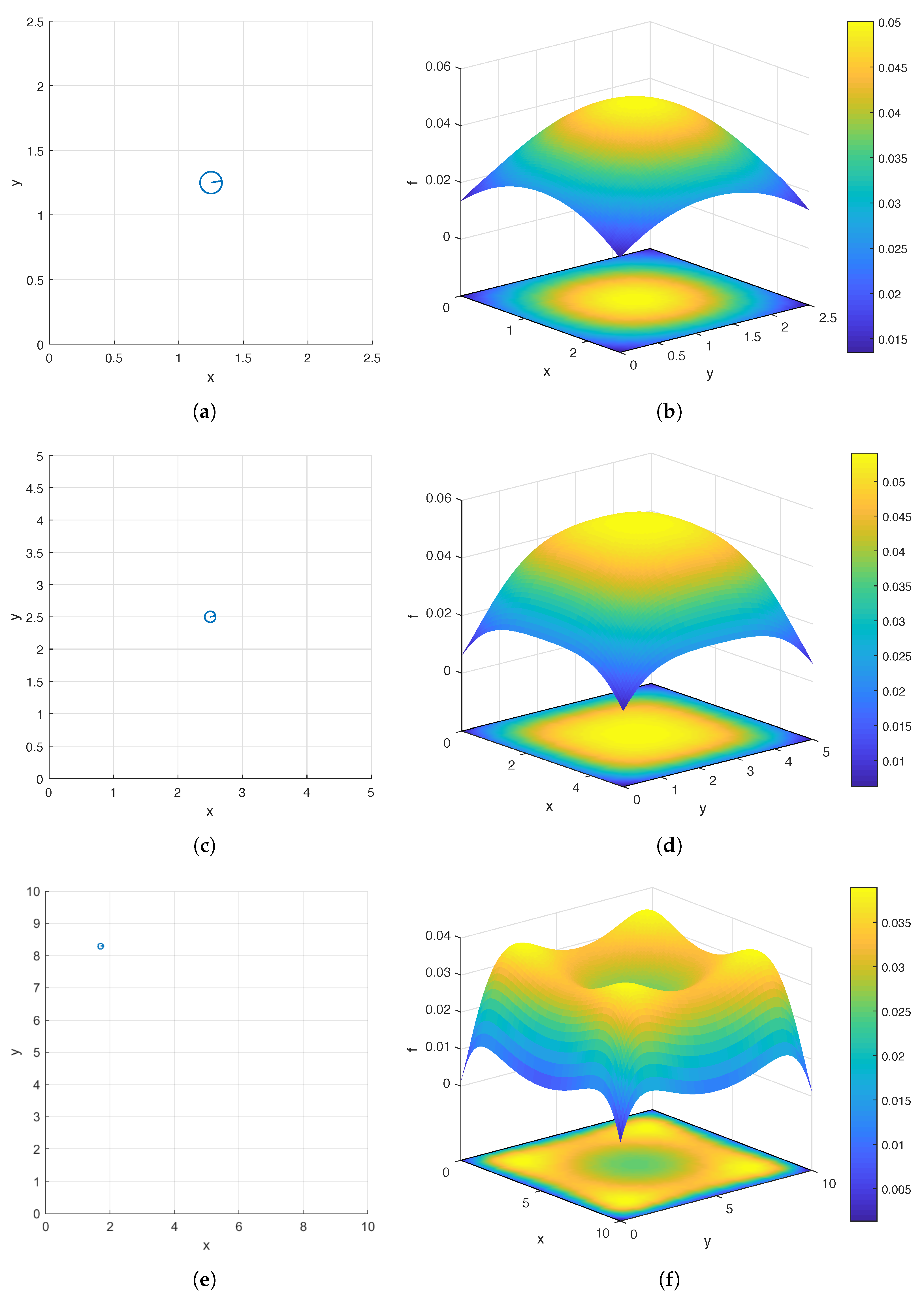
We consider a square flow meter defined by (
7) and three values of
W:
, 5, and 10. In
Figure 3b,d,f, we show the surface and contour plots of
over the domain
corresponding to
, 5, and 10, respectively. For each
W, in order to produce the pair of plots, we sample
f at the following uniformly distributed grid points:
As can be seen in
Figure 3b,d,f, for all three values of
W, global maximizers of
f lie on the diagonals of the domain. It is interesting to note that while the global maximizer is the center
of the domain and unique when
or 5, there are four global maximizers located near the four corners of the domain when
. While intuition might lead one to expect the center to be the global maximizer, in fact, it is a local minimizer when
, and the global maximum (
) is considerably larger than this local minimum (
). This clearly demonstrates the importance of quantitative analysis when searching for an optimal design of a bacterial carpet.
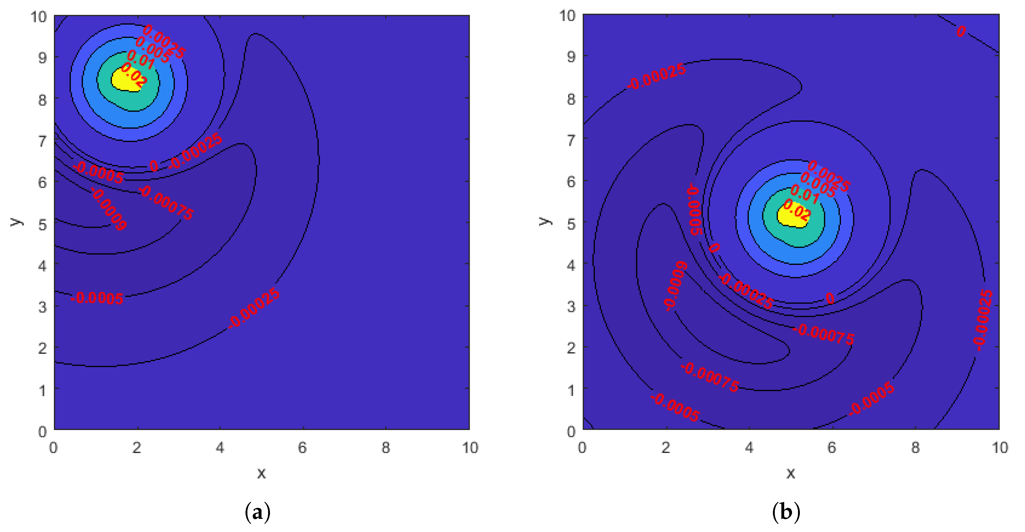
To further investigate why the optimal location of the helix is near the corners instead of the center of the domain when the width of the flow meter is 10, in
Figure 4, we draw the contour plots of the instantaneous
z-direction fluid velocity on the flow meter when the helix is based at one of the four optimal locations (
Figure 4a) and when it is based at the center of the domain (
Figure 4b). Comparing the two contour plots, we observe that when the helix is based at the center, a considerably larger region on the flow meter has small negative
z-direction velocity. More precisely, the areas enclosed by the level curves corresponding to
z-direction velocities
,
,
, and
in
Figure 4b are almost twice as large as their counterparts in
Figure 4a. In addition,
Figure 4 also helps explain why the optimal location of the helix is at the center when the width of the flow meter is
or 5: both flow meters are small enough that placing the helix at the center maximizes the region with large positive
z-direction velocity while creating no region or only a negligible region where the
z-direction velocity is negative.
We apply both the hybrid method described in
Section 2.4.3 and a GA to solve (
11) and compare their performance. In Step 1 of the hybrid method, we apply a GA to find a maximizer
of
, the surrogate model of
(see
Table 1 and
Table 2 for a comparison of the two functions); and in Step 2 of the hybrid method, we apply the BFGS algorithm with initial guess
to find a maximizer
of
. In
Table 3, we list the maximizers
and
found in the hybrid method for flow meters (
7) of widths
, 5, and 10. In
Figure 3a,c,e, we also display the top views of the optimal carpets corresponding to the three flow meters respectively.
Table 4 and
Table 5 contain the numbers of iterations, the numbers of function evaluations, and the runtimes of the hybrid method and a GA, respectively. We use MATLAB’s
ga function, an implementation of a GA, to find maximizers for both
and
. The default setting of
ga is used except that parallel computing is enabled and the range of the initial generation of candidate solutions is set to
. We note that GAs are not deterministic (see
Section 2.4.1). Thus, for reproducibility of the results presented in
Table 3,
Table 4 and
Table 5, we reset the seed of MATLAB’s random number generators to 0 using the command
rng default before calling the function
ga. We use MATLAB’s
fminunc function with its default setting, which implements the BFGS algorithm, to find a maximizer of
in Step 2 of the hybrid method (Both MATLAB functions
ga and
fminunc are for the minimization of a given objective function. Since we wish to maximize
or
instead, in our MATLAB implementation, we use
or
as the objective function).
As seen in
Table 4 and
Table 5, for all three flow meters, the hybrid method is significantly more efficient than the GA, requiring
less runtime. Although the GA requires about three thousand function evaluations to converge whether it is applied to
or
, since
is considerably cheaper to evaluate (see
Table 2), applying the GA to
is also considerably cheaper. In the hybrid method, once the estimate
is found by the GA in Step 1, the BFGS algorithm, which starts with
, converges quickly to the maximizer
in Step 2, requiring only two or three iterations and less than 20 function evaluations. Moreover, we can see that the hybrid method is more accurate than the GA by comparing the maximizers
and
found by the two methods, respectively (see
Table 3 and
Table 5). We also observe that the runtimes of both the hybrid method and GA increase with the size of the flow meter. Note that since the initial candidate solutions are randomly chosen in the GA, in the case where the flow meter is
, both the hybrid method and GA may find different maximizers in different runs if we do not reset the seed of the random number generators to the same number.
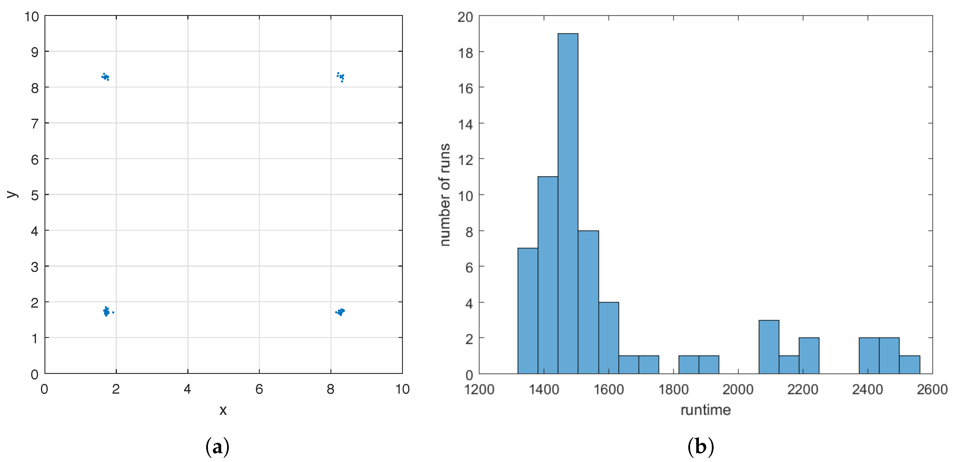
To demonstrate the robustness of the GA at finding a good initial guess in Step 1 of the hybrid method, for the case where the flow meter is
, we apply the GA to
sixty-four times and initialize the random number generators based on the current time using the command
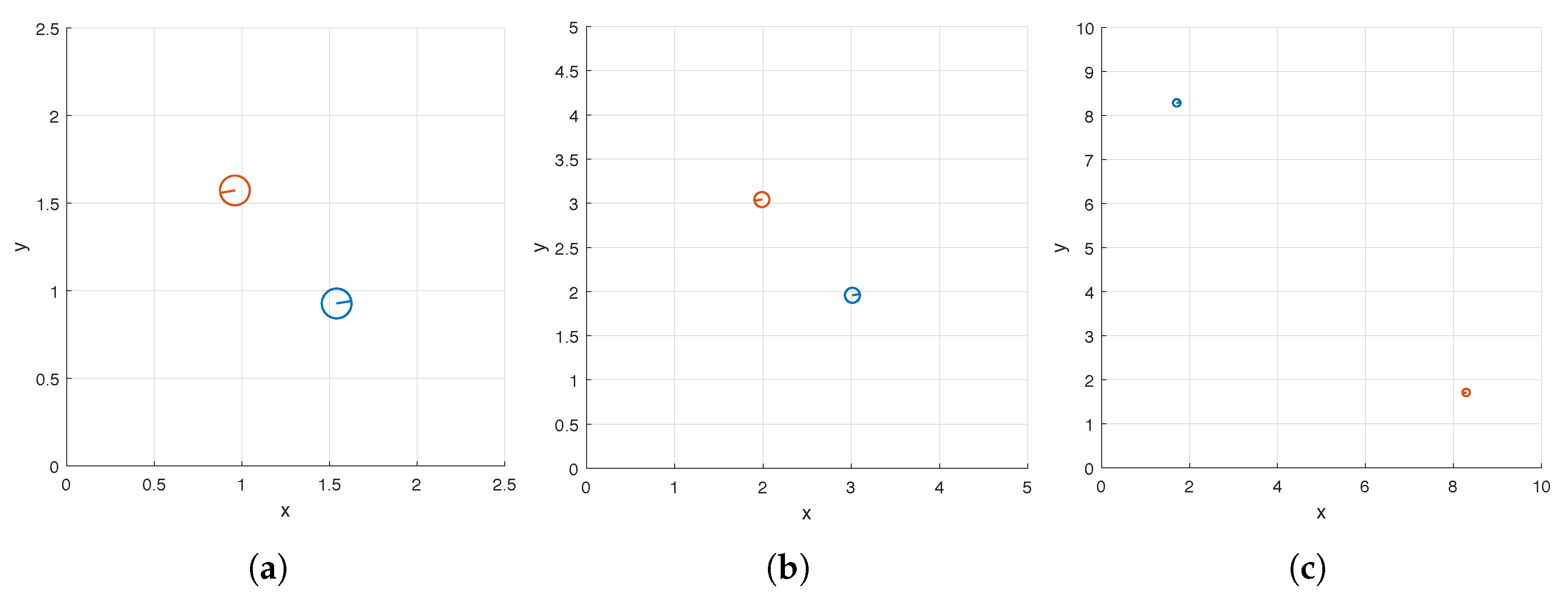
rng shuffle before each run. The GA uses a different sequence of random numbers in each run due to the re-initialization. In
Figure 5a, we display all sixty-four
’s found by the GA. They form four clusters around the four maximizers of
(see
Figure 3f), and the sizes of the clusters are 20, 19, 10, and 15. This demonstrates that the GA applied to
always finds an initial guess
close to one of the maximizers of
, although the maximizer may differ from run to run depending on the sequence of random numbers used. Runtime of the GA varies with the seed of the random number generators as well. In
Figure 5b, we show a histogram of the sixty-four runtimes, the majority of which is less than 1800 s.
3.2. A Pair of Helices
We now apply the hybrid method to find an optimal design of a carpet consisting of two helices for fluid pumping. We set the phase shift of the first helix to zero (
) and let the design parameters be the
coordinates of the base points of the two helices and the phase shift of the second helix. That is,
This optimization problem (
11) is significantly more difficult to solve than the one in
Section 3.1, not only because there are more design parameters (five instead of two) but also because the computational cost of evaluating
and
increases with the number of helices (see (
10)) as is shown in
Table 2.
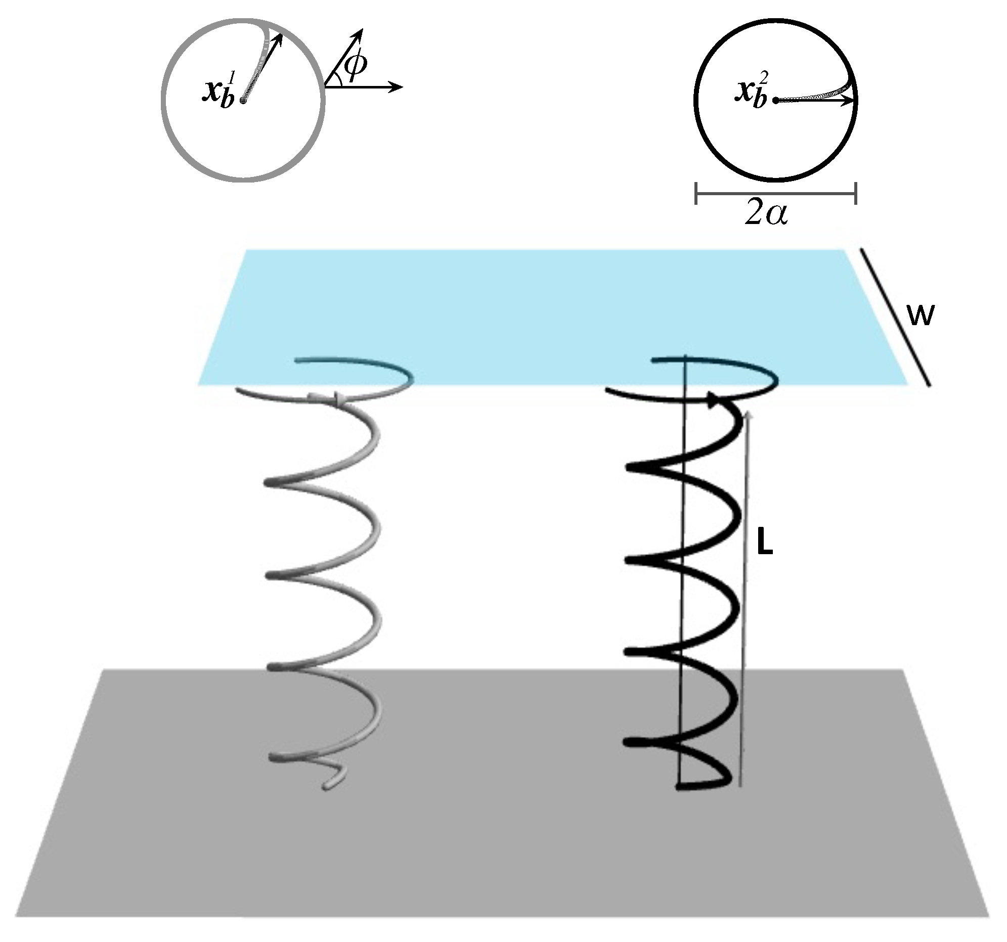
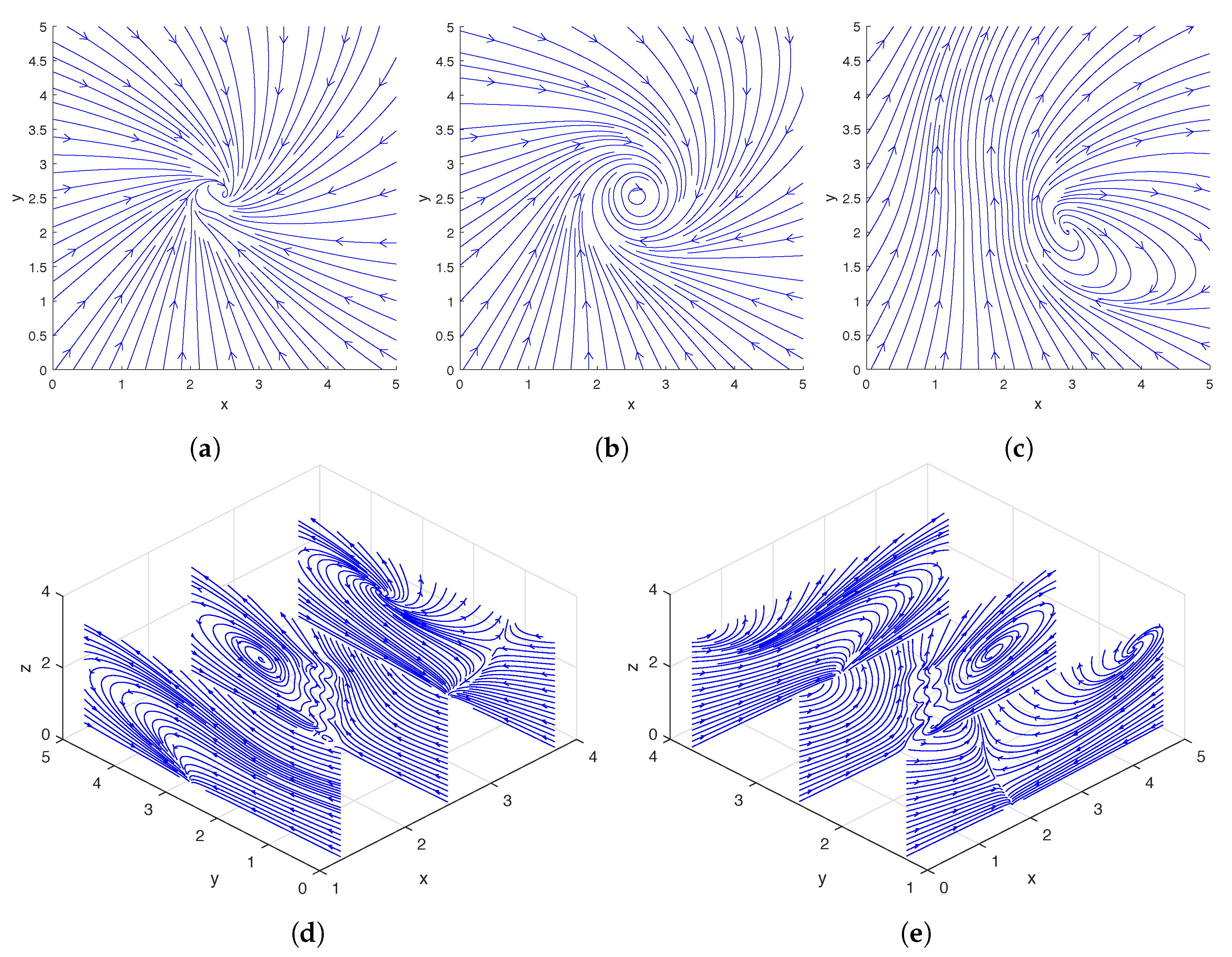
In
Figure 6, we show the streamlines drawn based on the instantaneous fluid velocity around a pair of rotating helices. As can be seen in
Figure 6d,e, the helices move the fluid near their tips upward while rotating. A more detailed analysis of the flow field around a pair of rotating helices can be found in [
13].
We again consider a square flow meter (
7) and three values of
W, as in
Section 3.1. The maximizers found by the hybrid method are listed in
Table 6 and the top views of the corresponding optimal carpets are displayed in
Figure 7. We use
to denote the maximizer of
found by the GA and
to denote the maximizer of
found by the BFGS algorithm using
as its initial guess. The iteration counts, numbers of function evaluations, and runtimes of the GA and BFGS algorithm are reported in
Table 7.
As can be seen in
Table 6 and
Figure 7, the hybrid method suggests that in order to maximize pumping, we should place the pair of helices along the diagonal of the domain
and set the phase shift of the second helix to
(recall that the phase shift of the first helix is fixed at 0). These results are consistent with what was observed in [
13] in that pumping was maximized when the difference between the phase shifts is
. However, we note that while this does maximize pumping, the distance between the optimal locations of the helices is sufficiently large so that when they are placed at these locations, the choice of phase shifts has a minimal impact on pumping. (For a pair of helices, the effect of the difference between their phase shifts on pumping has been studied in [
13], where they were placed at various distances apart.) This is similarly observed for the cases of three and four helices considered in
Section 3.3. We conjecture that the choice of phase shifts will play a greater role when the optimal locations of the helices are forced to be closer to one another, such as when there are more helices or when the flow meter is smaller.
Table 7 shows that, like in the case of a single helix, although a large number of iterations and function evaluations are needed for the GA to find the initial guess,
, once it is found, the BFGS algorithm only requires a relatively small number of iterations and function evaluations to converge to the maximizer,
. Additionally, the total runtime of the hybrid method increases with the size of the flow meter.
In the case with one helix, because we were optimizing over only two parameters, the
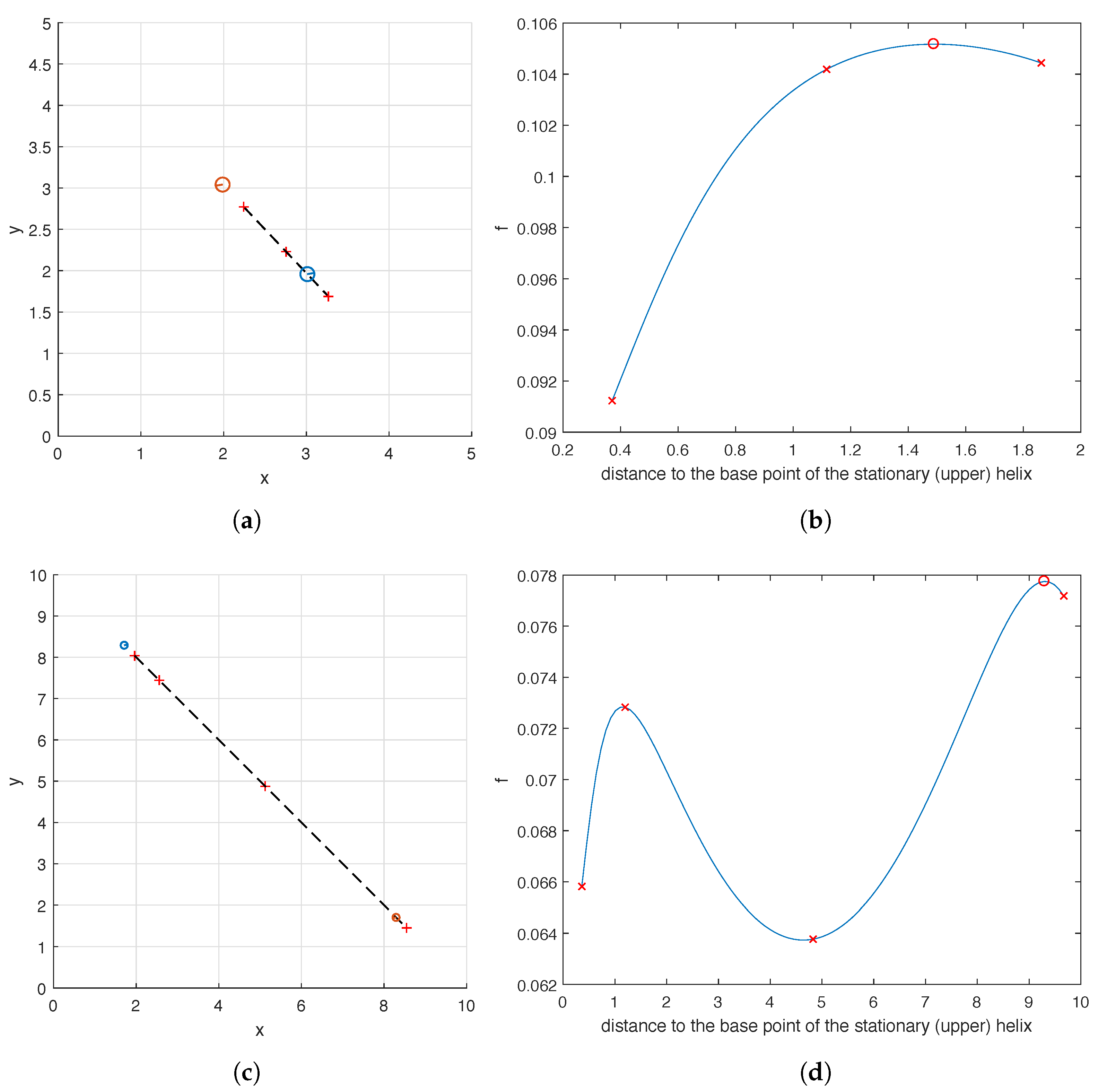
coordinates of the base of the helix, we could easily visualize the objective function. Now however, we are optimizing over five parameters (the base coordinates of each helix, and the phase shift of the second) so it is more difficult to visualize our objective function in a useful way. In order to investigate how the placement of the pair of helices affects the carpet’s performance at pumping, for the flow meters (
7) with widths
and 10, we fix the phase shifts of both helices, the location of one of the them and calculate
as the location of the other helix is varied. To be more precise, we fix all the design parameters of the optimal carpets shown in
Figure 7b,c except for the location of the lower helix. We then examine the value of
as we move the lower helix along the dashed line shown in
Figure 8a,c. This line goes through the base points
and
of the two helices in the optimal carpet found by the hybrid method. As can be seen in
Figure 8b, when
, the pumping capability of the carpet first grows as the distance increases, peaks as the moving helix reaches its optimal position
found by the hybrid method, and then starts to decline as the distance increases further. For the case
, the graph of
is quite similar and not shown here. As shown in
Figure 8d, the graph of
is even more interesting in the case of
. As the distance increases, the value of
first increases to reach a local maximum and then decreases to reach a local minimum, before it increases again to the global maximum when the moving helix is at its optimal position
calculated by the hybrid method. In
Figure 8, a few sample locations of the moving helix as well as the corresponding values of
are marked for reference.
3.3. Multiple Helices
We also apply the hybrid method to determine optimal designs that maximize pumping for carpets consisting of three and four helices. The design parameters are the
coordinates of the base points and phase shifts of the helices. (The phase shift of the first helix is fixed at 0, as in
Section 3.2). Thus, there are eight and eleven design parameters in these two cases respectively.
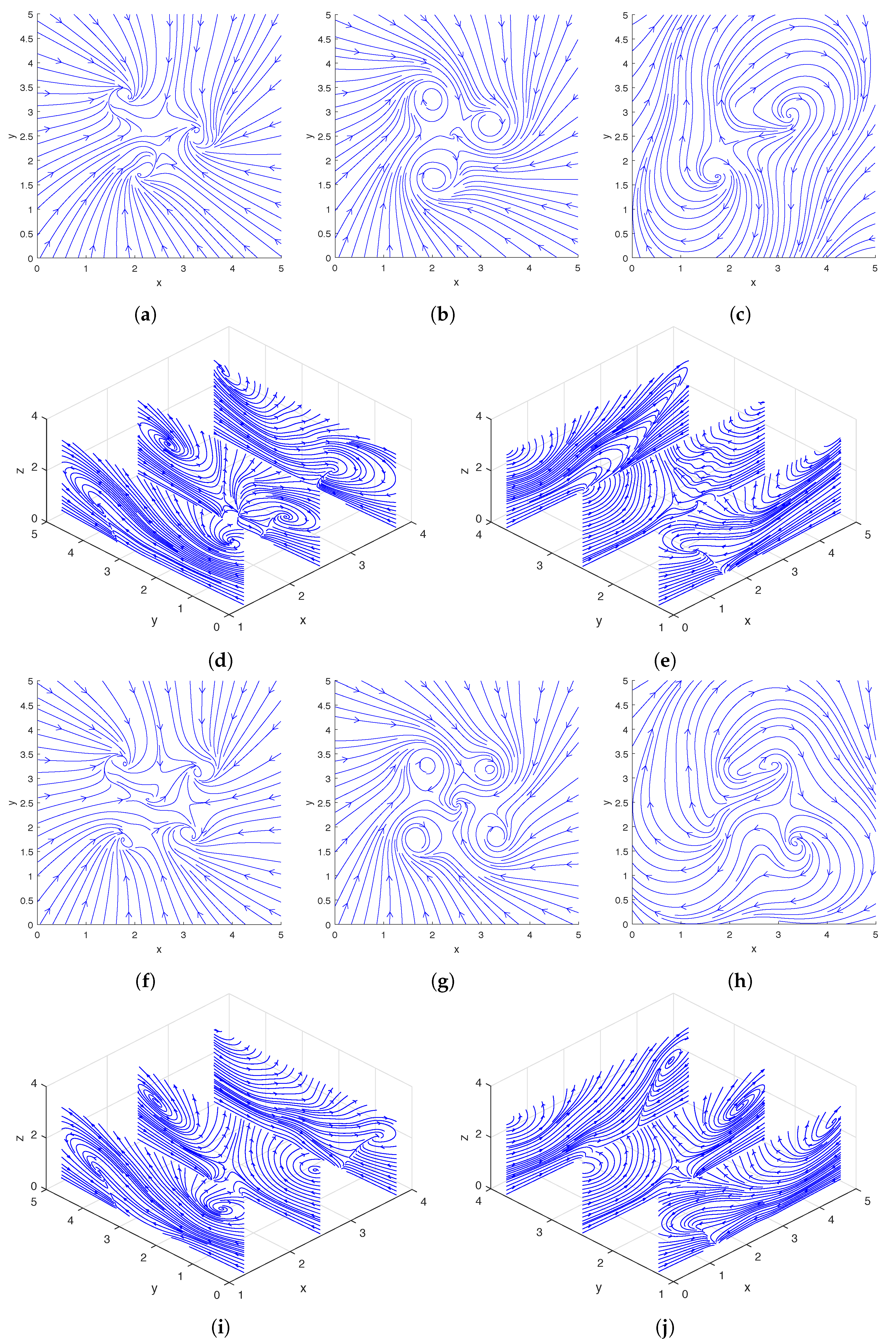
In the top two rows and bottom two rows of
Figure 9, we show the streamlines drawn based on the instantaneous fluid velocity around three and four rotating helices, respectively. As can be seen in
Figure 9d,e,i,j, the helices move the fluid near their tips upward while rotating.
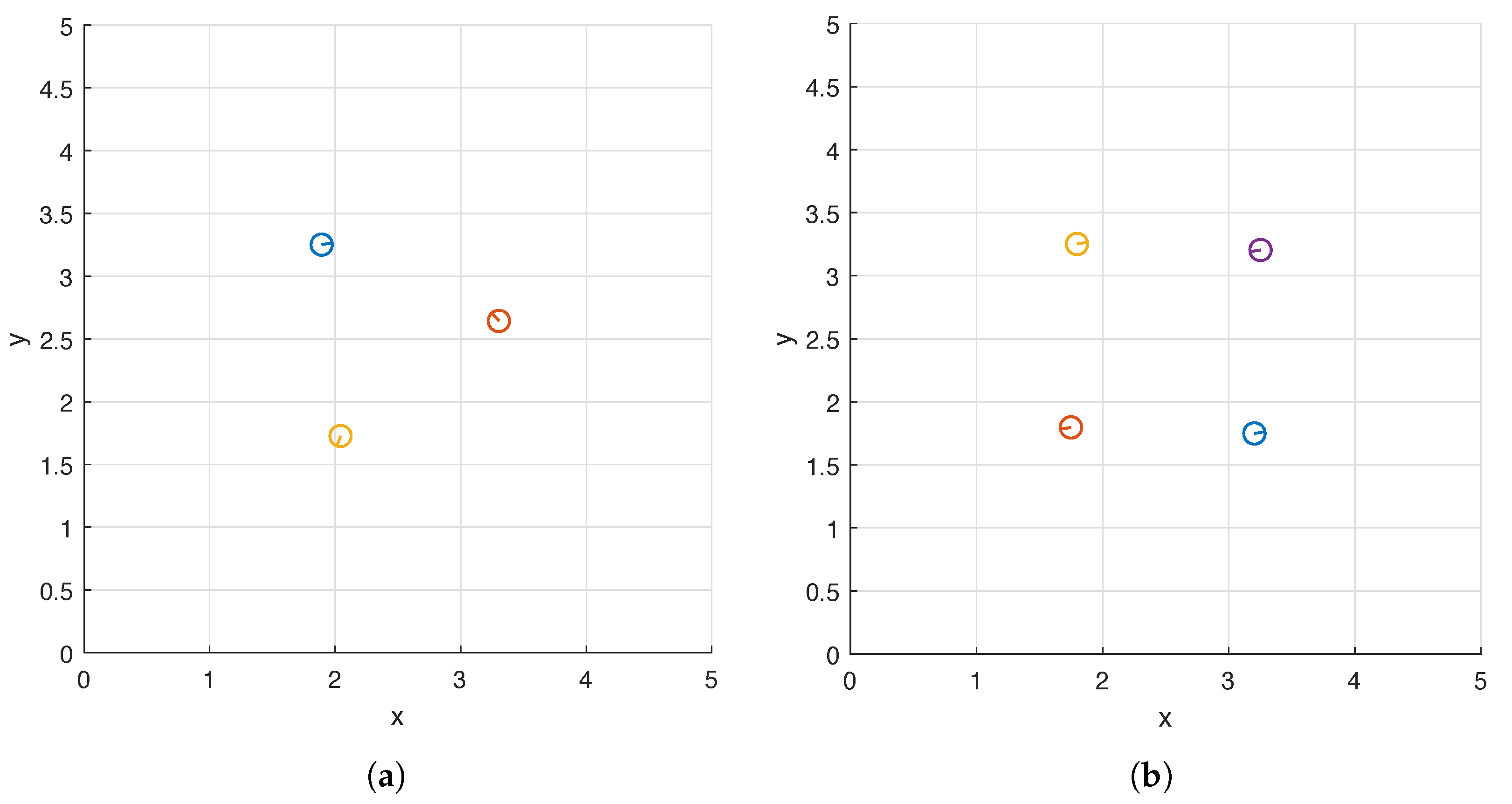
We again consider the square flow meter (
7) whose width is
and display the top views of the optimal carpets in
Figure 10. Interestingly, the helices approximately form an equilateral triangle when there are three of them (
Figure 10a) and a square when there are four (
Figure 10b) and both shapes are centered at
. The differences between the phase shifts of two helices located on adjacent vertices are
and
in the two cases respectively.
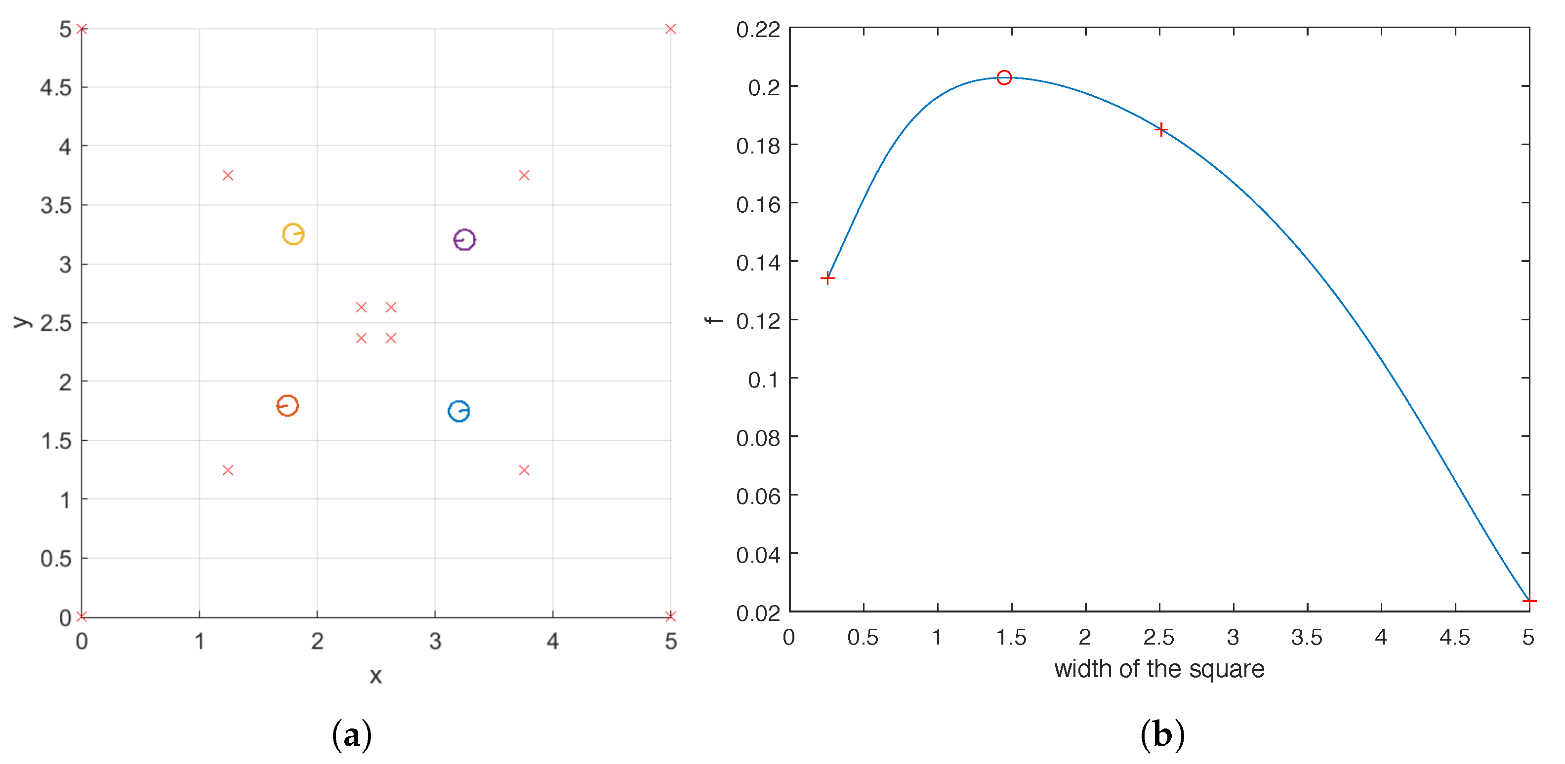
For the case of four helices, we also examine the objective function
for a family of carpets which includes the optimal one found by the hybrid method. They share the following properties: the base points of the four helices form a square centered at
, each of its four edges is parallel to the
x or
y axis, and the difference in the phase shifts of two helices located on adjacent vertices is
. In
Figure 11a, we illustrate three such carpets whose base points are marked by crosses. The optimal carpet found by the hybrid method is also plotted for reference. For this family of carpets, we plot the value of
against the width of the square in
Figure 11b, which indicates that as the square becomes larger, the ability of the carpet to pump first increases and then decreases, reaching its maximum at the width predicted by the hybrid method. One key observation can be made from
Figure 11 that when the four helices are uniformly distributed within the domain
, that is, when the width of the square is
, the pumping is sub-optimal. Once again, this shows that intuition does not necessarily lead to optimal carpet design.
In
Table 8, we report the numbers of iterations, numbers of function evaluations as well as runtimes of the hybrid method. Comparing
Table 4,
Table 7 and
Table 8, we note that the computational cost of the hybrid method increases progressively with the number of helices. This is again due to the growing number of design parameters and cost of evaluating
and
(see (
10) and
Table 2).


