A Model of Two Quantum Fluids for the Low Energy Excited States of the Systems with Entities That Mimic the Magnetic Monopoles

Abstract

The low energy excitation states in frustrated magnetic structures can generate quasiparticles that behave as if they were magnetic charges. These excited states produce, in the so-called spin-ice materials, two different peaks of specific heat at temperatures less than 1.5 K. In this paper, we consider that the first structure is caused by the formation of fluid of magnetic dipoles configured by the dumbbell model with a boson nature in consonance with that described by Witten for mesons. The second structure, wider than the first one, corresponds to a plasma state that comes from the breaking of a great number of dipoles, which provokes the appearance of free magnetic charges, which constitute a cool magnetic plasma fluid. In this paper, we determine thermodynamic analytical functions: the thermo-potential and internal energy and their respective derivative physical magnitudes: entropy, and magnetic specific heat. We obtain results in a good concordance with the experimental data, which allow us to explain the phase transitions occurred in these spin-ice materials at very low temperatures.

1. Introduction

At the present time, evidence of the existence of elementary particles with magnetic charges in a vacuum seems to be null both in high energy physics and in Cerenkov particles that come from outer cosmological space. Magnetic monopoles are theoretical conceptual objects introduced in high-energy theories to adjust the standard model and theories beyond it, which pursue the formulation of the possible great unification of the four forces of nature [1,2,3,4,5,6]. The pristine Dirac idea [1] of the existence of quantized magnetic charges, preconized by Dirac in 1931, has not been experimentally confirmed with any empirical evidence; only the known results of the Stanford experiment have been [7] presented as a possible indication of the monopole existence. Much more recently, Dusad et al. [8] may have been inspired by the Cabrera measurements, and some other experiments in pirocholore crystals [9,10,11,12,13,14] have recovered the squid superconductivity device for detecting entities that can be defined as magnetic monopoles” since their behavior mimic those associated with the magnetic charges.

Therefore, these entities arising from the excited magnetic states are not elementary particles in freedom but quasiparticle states within the matter. The behavior of these quasiparticles is as that of the magnetic charges. Consequently, henceforth, we will name these quasiparticles either magnetic charges or magnetic monopoles. In a recent paper [8], the authors report “the development flux noise spectrometer and measurements of the frequency and temperature dependence of magnetic-flux noise generated by Dy2Ti2O7 crystals”. These effects are justified by the presence of these cited quasiparticles whose behavior is as a fluid in a plasma-like state. Thirteen years ago, the recurrent issue of the existence of magnetic charges saw an important breakthrough, although in a different sense to that which Dirac, Hooft, and Poliakov and Cabrera attempted to design.

In the so-called “spin-ices”, structural modifications of the magnetic lattices produce excited global states, whose corresponding quasiparticles generate a bosonic particle condensation at very low temperatures. These quasiparticles are magnetic dipoles, which, under light increases of temperature, break, leaving in freedom the magnetic charges [11,12,13,14,15,16,17]. A theoretical model designed in 2008 [12] named the dumbbell model allows us to explain the low energy excitation states as quasi-free magnetic charges in the spin-ices.

These many-body states generated via increases of temperature are produced via spin-flips among contiguous tetrahedra, which constitute the well-known crystal structure of these materials [9,10,11,12,13,14,15,16,17,18,19,20,21,22,23]. The seminal idea is that the constitution of these excitation states creates both the magnetic dipoles and the free magnetic charges. These free magnetic charges are generated when the attractive interaction of Coulombian nature [18] between the two magnetic charges of the dipoles is broken via the increase in temperature. The existence of free magnetic charges in freedom and with kinetic energy [12,13] constitutes the cool magnetic plasma.

Moreover, at present time, several artificial structures manifest similarities with magnetic charges at ligth higher temperatures. Additionally, other different structures as the topological insulators [24] present image states, which can be conceived as dyons and systems within artificial magnetic fields [25]. All these cited cases present a rich phenomenology due to the possibility of movement of the magnetic charges: movement that can be produced by a magnetic field in its own parallel direction, which can be treated as a magnetohydrodynamic fluid when the density of magnetic monopoles is great enough.

In all these scenarios, the constant volume specific heat and the magnetic susceptibility [26,27,28,29,30,31,32,33,34] have been measured. These experimental results allow us to compare our theoretical results with the experimental data, as well as to give consistency to nature regarding the phase transitions occurred in these compounds approximately between 0.08 and 1 kelvin. On the other hand, some relatively recent experiments in changes in the speed of sound have been interpreted as the existence of a possible phase transition of the first kind [35] in these spin-ice systems. As usual in these transitions, entropy and specific heat can undergo anomalies, which implies a coexistence of two phases without changing temperature. In the specific heat measurements, two clear peaks appear in the experimental results. The first peak is presented at a very low temperature, and it appears in the initial tenths of kelvin which may be coherent with the existence of a bosonic condensation. The other peak, wider than the first, announces an increase in free magnetic charges, which constitute a clear magnetic plasma state with null total charge.

We analyze these structures of excited states by means of a pseudospin symmetry model in a certain phenomenological similarity to that existing in hadronic mesons [36]. These bosons that configure a condensate as an excited global state at the lowest temperature are responsible for the first peak in the specific heat. Each of these bosons are a linear combination of a quantum superposition, of s = 0 and s = 1 states consisting of pole–antipole dimers [37,38,39,40,41,42,43,44]. These dimers can break when the temperature rises and leave two free charges for each of the dipoles, which constitute a magnetic plasma [45] that is responsible for the peak that is the second widest and of less intensity in the specific heat. The model described in this paper has been inspired, on one hand, by the works published by Itoh et al. [37], in which a fermion nature is assigned to the magnetic monopoles, and on the other hand, by Witten [36], who established the analogy between the magnetic pole–antipole pairs with the hadronic mesons. However, although the inspiration in Witten‘s paper is clear, we recognize the differences in the two cases as well as the possible similarities. For instance, there are differences between the relativistic particle plasmas with respect to those studied here, which concern effective magnetic charges. One of these differences is that, in the case of charged particles in relativistic plasmas, a Bose–Einstein condensate arises due to photons that can induce a mass effect [46]. These photons come from the electromagnetic interactions between the relativistic charges. The authors “show that photon condensation is possible in an unbounded plasma because, in contrast with other optical media, plasmas introduce an effective photon mass”. Meanwhile, in this case of the spin-ices, the plasma is produced when each magnetic dipole of the bosonic condensation is broken into two free charges: a positive charge and a negative charge. Therefore, the plasma is generated when the magnetic bosonic condensation disappears and is converted in a magnetic and cool neutral plasma state [45].

2. Hamiltonian and Isospin Structure

There have been many keys for a long time with which we can justify the plausibility of the fermionic character of the magnetic monopoles and, in turn, the bosonic for the magnetic dipoles coming from the dumbbell model [12]. We can consider the intuitions of high-energy physicists such as Hootf [3] and Polyakov [4] working 50 years or more ago; 25 years ago, Witten [36]; and even more recently, Itoh et al. [37], each of whom can give support our analysis. In addition, some experimental studies have obtained data compatible with the fermionic nature of the monopoles and the bosonic nature of the dipoles evidenced via the coherence of theoretical results with the experimental ones. These experimental results and those intuitions endorse the assignment of this spin nature to the one-body components of the excited low energy many-body states within the materials called spin-ices. In addition, the inclusion of this pseudospin character in the individual states substituting the magnetic structures in virtue of the dumbbell model allow us to obtain free energies or thermodynamic potentials using the Bose–Einstein and Fermi Dirac statistics for the individual components of the global excitation states of lowest energy. These thermodynamic potentials or Helmholtz functions lead us to results of the entropy and specific heat corresponding to these magnetic entities, which can be fitted to the experimental data obtained over the last 13 years. We start from the following formulation of a many-body Hamiltonian, already used in our previous paper of 2018 [47]:

$$\mathbf{H} = {\mathbf{H}}_{\mathbf{0}} + {\mathbf{H}}_{\mathbf{I}} = {\displaystyle \sum _{\mathbf{j}}}\left(\mathsf{\epsilon }{\prime }_{\mathbf{j}} - \mathsf{\mu }\right)\left({\mathbf{p}}_{\mathbf{j}}^{†}{\mathbf{p}}_{\mathbf{j}} + {\mathbf{a}}_{\mathbf{j}}^{†}{\mathbf{a}}_{\mathbf{j}}\right) + {\displaystyle \sum _{\mathbf{i}\mathbf{j}}{\mathbf{V}}_{\mathbf{i}\mathbf{j}}}{\mathbf{p}}_{\mathbf{j}}^{†}{\mathbf{a}}_{\mathbf{j}}^{†}{\mathbf{a}}_{\mathbf{i}}{\mathbf{p}}_{\mathbf{i}} + \mathbf{U}{\displaystyle \sum _{\mathbf{i}}{\mathbf{n}}_{\mathbf{i}}^{\mathbf{p}}}{\mathbf{n}}_{\mathbf{i}}^{\prime \mathbf{p}} + \mathbf{U}{\displaystyle \sum _{\mathbf{i}}{\mathbf{n}}_{\mathbf{i}}^{\mathbf{a}}}{\mathbf{n}}_{\mathbf{i}}^{\prime \mathbf{a}}$$

(1)

where ${\mathbf{H}}_{\mathbf{0}}$ is the Hamiltonian of the non-interacting system; $\mathsf{\epsilon }{\prime }_{\mathbf{j}}$ is the energy for a magnetic charge in the j site of the magnetic structure whose energy is given below in Equation (2); $\mathsf{\mu }$ is the chemical potential; ${\mathbf{p}}_{\mathbf{j}}^{†}({\mathbf{p}}_{\mathbf{j}})$ is a creation (annihilation) operator of a positive magnetic charge and ${\mathbf{a}}_{\mathbf{j}}^{†}({\mathbf{a}}_{\mathbf{j}})$ is a creation (annihilation) operator of a negative magnetic charge; ${\mathbf{H}}_{\mathbf{I}}$ is the interaction Hamiltonian, where the first term of ${\mathbf{H}}_{\mathbf{I}}$ is the interaction between the magnetic charges of the dumbbell-type magnetic dipoles located in two different contiguous tetrahedra of the crystal structure of the spin-ices; and the $\mathbf{U}$ of the two Hubbard-like terms is the repulsive interaction among two charges of the same sign located in the same tetrahedron. Correspondingly, we have the following commutation rules, $\left[{\mathbf{H}}_{\mathbf{0}},{\mathbf{S}}_{\mathbf{z}}\right] = \left[{\mathbf{H}}_{\mathbf{0}},{\mathbf{S}}^{\mathbf{2}}\right] = \mathbf{0}$ and the corresponding algebraic relations $\left\{{\mathbf{a}}_{\mathbf{i}}^{†},{\mathbf{a}}_{\mathbf{j}}^{†}\right\} = \left\{{\mathbf{p}}_{\mathbf{i}}^{†},{\mathbf{p}}_{\mathbf{j}}^{†}\right\} = \mathbf{0}$ and $\left\{{\mathbf{a}}_{\mathbf{i}},{\mathbf{a}}_{\mathbf{j}}^{†}\right\} = \left\{{\mathbf{p}}_{\mathbf{i}},{\mathbf{p}}_{\mathbf{j}}^{†}\right\} = {\delta }_{\mathbf{i}\mathbf{j}}$. Therefore, we consider the following definitions for the monopole states of positive magnetic charges as fermionic individual states: ${\mathbf{p}}_{\mathbf{i}}\left|\mathbf{0}\right.〉 = \mathbf{0}$; ${\mathbf{p}}_{\mathbf{i}}^{†}\left|\mathbf{0}\right.〉 = \left|{\mathbf{p}}_{\mathbf{i}}\right.〉 = \left|\frac{\mathbf{1}}{\mathbf{2}}\mathbf{,}\frac{\mathbf{1}}{\mathbf{2}}\right.〉$; and negative magnetic charge ${\mathbf{a}}_{\mathbf{i}}\left|\mathbf{0}\right.〉 = \mathbf{0}$${\mathbf{a}}_{\mathbf{i}}^{†}\left|\mathbf{0}\right.〉 = \left|{\mathbf{a}}_{\mathbf{i}}\right.〉 = \left|\frac{\mathbf{1}}{\mathbf{2}}\mathbf{,}-\frac{\mathbf{1}}{\mathbf{2}}\right.〉$. Concerning the bosonic dipoles states, we define ${\mathbf{p}}_{\mathbf{i}}^{†}{\mathbf{a}}_{\mathbf{i}}^{†}\left|\mathbf{0}\right.〉 = \left|{\mathbf{p}}_{\mathbf{i}}{\mathbf{a}}_{\mathbf{i}}\right.〉 = -\left|{\mathbf{a}}_{\mathbf{i}}{\mathbf{p}}_{\mathbf{i}}\right.〉 = \frac{\sqrt{\mathbf{2}}}{\mathbf{2}}\left({\left|\mathbf{0},\mathbf{0}\right.〉}_{\mathbf{i}} + {\left|\mathbf{1},\mathbf{0}\right.〉}_{\mathbf{i}}\right)$, whose singlet state is ${\left|\mathbf{0},\mathbf{0}\right.〉}_{\mathbf{i}} = \frac{\mathbf{1}}{\sqrt{\mathbf{2}}}\left(\left|{\mathbf{p}}_{\mathbf{i}}{\mathbf{a}}_{\mathbf{i}}\right.〉-\left|{\mathbf{a}}_{\mathbf{i}}{\mathbf{p}}_{\mathbf{i}}\right.〉\right)$, and the triplet state is ${\left|\mathbf{1},\mathbf{0}\right.〉}_{\mathbf{i}} = \frac{\mathbf{1}}{\sqrt{\mathbf{2}}}\left(\left|{\mathbf{p}}_{\mathbf{i}}{\mathbf{a}}_{\mathbf{i}}\right.〉 + \left|{\mathbf{a}}_{\mathbf{i}}{\mathbf{p}}_{\mathbf{i}}\right.〉\right)$; ${\left|\mathbf{1},\mathbf{1}\right.〉}_{\mathbf{i}} = \left|{\mathbf{p}}_{\mathbf{i}}{\mathbf{p}}_{\mathbf{i}}^{,}\right.〉$ and ${\left|\mathbf{1},-\mathbf{1}\right.〉}_{\mathbf{i}} = \left|{\mathbf{a}}_{\mathbf{i}}{\mathbf{a}}_{\mathbf{i}}^{,}\right.〉$. These two latter triplet states correspond to the existence of two magnetic charges of the same sign within the same tetrahedron and are energetically displaced by the positive high energy $\mathbf{U}$ of the two Hubbard-like terms of ${\mathbf{H}}_{\mathbf{I}}$.

In a first step, we do consider the energy of a dipole state when a vertex between two contiguous tetrahedra is produced by a spin flip; therefore, we have two magnetic charges, one in each of these two tetrahedra. This energy was calculated in reference [47,48].

$$\mathsf{\epsilon }{\prime }_{\mathbf{j}} = \mathbf{2}{\mathbf{K}}_{\mathbf{B}}\mathbf{T}\mathbf{l}\mathbf{n}\frac{{\mathbf{n}}_{\mathbf{0}}}{{\mathbf{n}}_{\mathbf{j}}} + \frac{\mathbf{2}{\mathbf{g}}_{\mathbf{j}}{\mathbf{\varphi }}_{\mathbf{0}}}{{\mathbf{T}}_{\mathbf{V}}}\mathbf{T} - \frac{{\mathsf{\mu }}_{\mathbf{0}}{\mathsf{\mu }}_{\mathbf{r}}{\mathbf{g}}_{\mathbf{j}}^{\mathbf{2}}}{\mathbf{4}\mathbf{\pi }\mathbf{d}} + {\mathsf{\sum }}_{\mathbf{0}}$$

(2)

where the third term on the right hand side of equality is the part of energy corresponding to the interaction among the magnetic charges of each dipole; ${\mathbf{g}}_{\mathbf{j}}$ is the magnetic charge of any tetrahedron; ${\mathbf{n}}_{\mathbf{0}}$ is the probability of the appearance of a magnetic charge in each tetrahedron for the ${\mathbf{T}}_{\mathbf{V}}$ temperature (this data can be obtained from the experimental data); ${\mathsf{\sum }}_{\mathbf{0}}$ is the necessary energy for obtaining a spin flip, which is the cause of the appearance of a magnetic charge at the temperature of the first peaks of the two magnetic charges of the magnetic dipole; ${\mathbf{T}}_{\mathbf{V}}$ is the experimental temperature of the first peaks in the specific heat [26,27,28,29,30,31,32,33,34]; ${\mathbf{\varphi }}_{\mathbf{0}}$(${\mathbf{n}}_{\mathbf{0}}$) is the magnetic potential (magnetic charge number) at ${\mathbf{T}}_{\mathbf{V}}$ temperature (see previous paper of 2018 in [47]); ${\mathbf{n}}_{\mathbf{j}}$ is the probability of the presence of a spin flip in the j vertex of two contiguous tetrahedra; and $\frac{{\mathsf{\mu }}_{\mathbf{0}}{\mathsf{\mu }}_{\mathbf{r}}{\mathbf{g}}_{\mathbf{j}}^{\mathbf{2}}}{\mathbf{4}\pi \mathbf{d}}$ is the first order perturbation energy due to the negative interaction of magnetic charges of different signs [47,48].

With the individual energy of the interacting magnetic charges of the Hamiltonian 1, we define the thermodynamic potential for the bosonic global state that is responsible the first peaks in the specific heat. This Helmholtz thermodynamic function [42,43,44] is the following:

$${\mathbf{F}}_{\mathbf{B}\mathbf{E}\mathbf{C}} = {\mathbf{K}}_{\mathbf{B}}\mathbf{T}{\displaystyle \sum _{\mathbf{j}}}\mathbf{ln}\left[\mathbf{1} - \mathbf{exp}\left(-\mathbf{ln}{\left(\frac{{\mathbf{n}}_{\mathbf{0}}}{{\mathbf{n}}_{\mathbf{j}}}\right)}^{\mathbf{2}} - \frac{\mathbf{2}{\mathbf{g}}_{\mathbf{j}}{\mathbf{\varphi }}_{\mathbf{0}}}{{\mathbf{K}}_{\mathbf{B}}{\mathbf{T}}_{\mathbf{V}}} - \frac{{\mathsf{\sum }}_{\mathbf{0}} - \mathsf{\mu }}{{\mathbf{K}}_{\mathbf{B}}\mathbf{T}} + \frac{\mathbf{1}}{{\mathbf{K}}_{\mathbf{B}}\mathbf{T}}\frac{{\mathsf{\mu }}_{\mathbf{0}}{\mathsf{\mu }}_{\mathbf{r}}{\mathbf{g}}_{\mathbf{j}}^{\mathbf{2}}}{\mathbf{4}\pi \mathbf{d}}\right)\right]$$

(3)

Further, if we extend expression (3) to a continuum version, the free energy per dipole is:

$${\mathbf{f}}_{\mathbf{B}\mathbf{E}\mathbf{C}} = \frac{{\mathbf{F}}_{\mathbf{B}\mathbf{E}\mathbf{C}}}{\mathbf{N}{\mathbf{n}}_{\mathbf{0}}} = \frac{\mathbf{1}}{{\mathbf{n}}_{\mathbf{0}}\mathsf{\beta }}{\displaystyle {\int }_{\mathbf{o}}^{\mathbf{1}}}\mathbf{ln}\left(\mathbf{1} - {\mathbf{t}}^{\mathbf{2}}{\mathbf{z}}_{\mathbf{1}}\right)\mathbf{d}\mathbf{t}$$

(4)

$${\mathbf{z}}_{\mathbf{1}} = \mathbf{exp}(-\mathsf{\theta })\mathbf{exp}(-\mathsf{\beta }\mathbf{b}),$$

(5)

where $\mathsf{\beta } = {\left({\mathbf{K}}_{\mathbf{B}}\mathbf{T}\right)}^{-\mathbf{1}}$; $\mathsf{\theta } = \frac{\mathbf{2}{\mathbf{g}}_{\mathbf{j}}{\mathbf{\varphi }}_{\mathbf{0}}}{{\mathbf{K}}_{\mathbf{B}}{\mathbf{T}}_{\mathbf{V}}}$;$\mathbf{b} = -\frac{{\mathsf{\mu }}_{\mathbf{0}}{\mathsf{\mu }}_{\mathbf{r}}{\mathbf{g}}_{\mathbf{j}}^{\mathbf{2}}}{\mathbf{4}\pi \mathbf{d}} + {\mathsf{\sum }}_{\mathbf{0}}-\mathsf{\mu }$; and $\mathbf{N}$ is the total number of vertices liable to undergo a spin inversion in the crystal structure. The parameter $\mathsf{\theta }$ establishes the relationship between the interaction energy of the local magnetic potential with the magnetic charges (defined in reference [47]) and the thermal energy at which the excited state of lowest energy has the first peak in the specific heat. Energy $\mathbf{b}$ contains three terms: the pole–antipole attraction energy determined by a perturbation way; −$\frac{{\mathsf{\mu }}_{\mathbf{0}}{\mathsf{\mu }}_{\mathbf{r}}{\mathbf{g}}_{\mathbf{j}}^{\mathbf{2}}}{\mathbf{4}\pi \mathbf{d}}$, the energy necessary for the formation of a magnetic charge by means of spin flip; ${\mathsf{\sum }}_{\mathbf{0}}$, defined in the dumbbell model [11] and the chemical potential, $\mathsf{\mu }$. In this latter expression, ${\mathsf{\mu }}_{\mathbf{r}}$ is the dressed local magnetic response of the global system over the interaction of the components of a generic magnetic dipole formed by a spin flip. This many-body magnetic response can be obtained via the perturbation theory.

However, in the beginning, we can and should consider a first perturbation order, considering the bare interaction, since we believe that—for the sake of simplicity—we can obtain it as promising guidance to fit the model in the most simplified format of perturbative theory. These perturbative theories of higher orders, even of an infinite order, such as those in Dyson’s equations, are often difficult, in computational time, to address without knowing the results of first order perturbative theories. Once we know the results of these, we can direct our efforts in more sophisticated perturbation theories such as the T-reaction matrix or those from the RPA (random phase approximation), both procedures being adjustable to the structure of Hamiltonian 1. Another possibility is to apply the perturbative theory to the definition of the thermodynamic potential of Equation (3) (see, for instance, ref. [42,43,44]).

3. Results on the Bosonic Condensation State

When spin flips produce the existence of magnetic dipoles, conceived as established by the dumbbell model, the term of interaction of Equation (1) favors the existence of a bosonic condensation, such as has been published in other research [47,48]. Such condensation can be analyzed by the thermodynamic potential that defines a global state, whose components, $\left|{\mathbf{p}}_{\mathbf{i}}{\mathbf{a}}_{\mathbf{i}}\right.〉 = \frac{\sqrt{\mathbf{2}}}{\mathbf{2}}\left({\left|\mathbf{0},\mathbf{0}\right.〉}_{\mathbf{i}} + {\left|\mathbf{1},\mathbf{0}\right.〉}_{\mathbf{i}}\right)$, are a quantum composition of spin 0 and spin 1 bosonic states. This point of diversification of different spin channels for this condensation is analyzed in some spin-ice materials. These s and p channels can be characterized by the individual states of the magnetic dimers that form the dipoles with individual wavefunctions $\left|{\mathbf{p}}_{\mathbf{i}}{\mathbf{a}}_{\mathbf{i}}\right.〉$. For this, we will consider the crystalline coherence that all the equivalent vertices of the magnetic structure have the same probability of generating a spin flip when a slight increase in temperature is present. Each global state will have a number, $\mathbf{N}\mathbf{n}$ magnetic dipoles, with $\mathbf{n}$ indicating the probability of presenting dipoles in each vertex identic within the crystalline structure. This probability varies from 0 to the value of ${\mathbf{n}}_{\mathbf{0}}$ that is reached at the temperature at which the specific heat presents the first peak. We can obtain from Expression 4, the analytical form of the thermodynamic potential. With this free energy, we determined, by means of its first and second derivatives, the entropy, ${\mathbf{s}}_{{}_{\mathbf{B}\mathbf{E}\mathbf{C}}} = -\frac{\partial {\mathbf{f}}_{\mathbf{B}\mathbf{E}\mathbf{C}}}{\partial \mathbf{T}}$ and specific heat,${\mathbf{c}}_{\mathbf{B}\mathbf{E}\mathbf{C}} = -\mathbf{T}\frac{{\partial }^{\mathbf{2}}{\mathbf{f}}_{\mathbf{B}\mathbf{E}\mathbf{C}}}{\partial {\mathbf{T}}^{\mathbf{2}}}$ and also as a first derivative respect to T of the internal energy. All these thermodynamic magnitudes are given in Figure 1 and Figure 2.

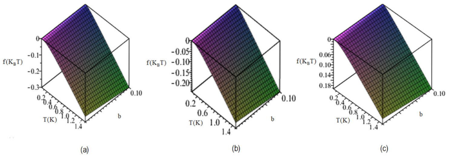
In the results of Figure 1, we give the evolution with the temperature of the thermodynamic potential. The evolution of this f-potential allows us to determine the other thermodynamical functions, the specific heat and entropy whose characteristic features give information about the phase transitions. This evolution with temperature has the following main characteristic features: (1) the values of the Helmholtz function are obviously negative and decreasing with increasing temperature; (2) the smaller the value of $\mathbf{b}$ energy, the greater the absolute value of the thermodynamic potential for any temperature, i.e., the absolute value of thermodynamic potential increases when the value of $\mathbf{b}$ energy decreases; (3) the greater the $\mathbf{b}$ energy, the greater the interval of temperature in which the f potential is zero and this f-function is zero at zero K. (4) This interval is between approximately 0 and 0.15 K for $\mathbf{b}$ energy between 0.1 and 0.25, which is the variation in $\mathbf{b}$ in the corresponding axis of Figure 1. This supports the fact that this value, $\mathbf{b}$ = 0.1, can be the one that yields better results for the thermodynamic functions. However, the other values of $\mathbf{b}$ energy should be also taken into account, since they can give results in agreement with other experimental data.

This behavior of f-potential, represented in Figure 1, is an important result and is clearly supported by the results generated in the thermodynamic functions derived from this Helmholtz free energy. The temperature evolution of f-potential is crucial for the appearance of a phase transition between 0.09 and 0.15 K. This phase transition was analyzed in a previous paper [47], in which we define it as a bosonic condensation which can be in restricted conditions a Bose–Einstein condensate phase transition. This BEC nature of this low energy excitation state is sensibly manifested in the other thermodynamic functions.

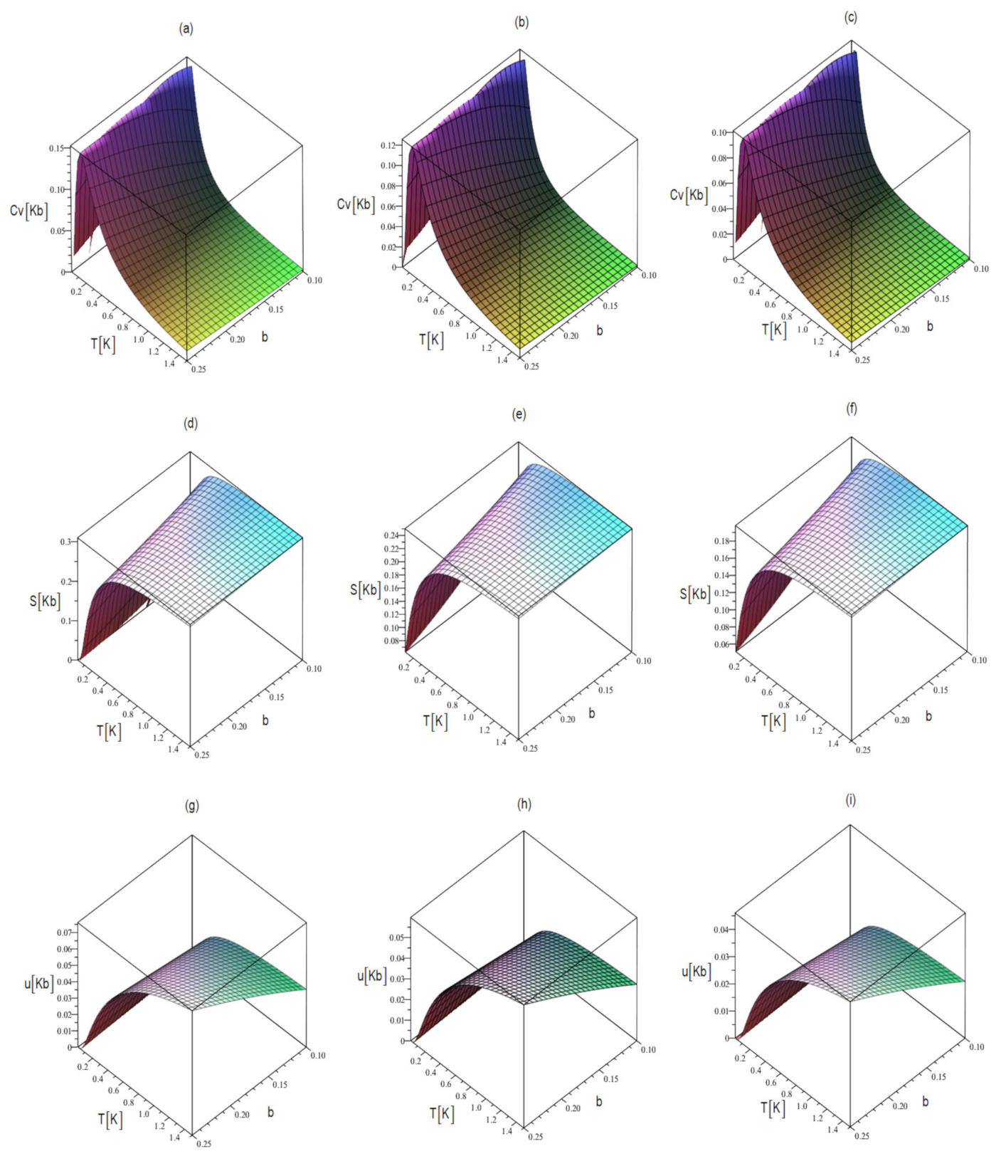
In Figure 2, we give entropy, specific heat, and internal energy for each pole–antipole pair, such as it happens in the elementary particles of meson nature [36]. This is calculated using Equations (2)–(5). In these plots, the coordinate axes of the z = 0 plane of the parallelepiped are the temperature and the parameter $\mathbf{b}$ and z axis is represented the corresponding thermodynamic magnitude. All these results of Figure 2 are obtained from the thermodynamic potential of the bosonic nature (Equation (4)).

The results of the three thermodynamic functions of Figure 2 are correlated, and they are all performed with the same parameters. These parameters are $\mathsf{\theta } = \mathbf{0.625}$ for Figure 2a–c; $\mathsf{\theta } = \mathbf{0.80}$ for Figure 2d–f; and $\mathsf{\theta } = \mathbf{1.00}$ for Figure 2g–i. The $\mathbf{b}$ energy varies in the interval, as in Figure 1, where $\mathbf{0.1}\le \mathbf{b}\le \mathbf{0.25}$. On the other hand, in the specific heat curves given in Figure 2a–c, we obtain the characteristic narrow peak that is detected experimentally, and the temperatures that appear at these peaks in our results are in reasonable concordance with the experimental data [26,27,28,29,30,31,32,33,34]. Another aspect of the specific heat results that deserves to be highlighted is that the smallest maximum is found at lower temperatures when the value of $\mathbf{b}$ energy decreases, although the intensity of the peaks is almost constant in the function of the $\mathbf{b}$ energy value. The entropy is given in Figure 2d–f in a three-dimensional graph whose axes have the same meaning as in Figure 2a–c. There is a perfect correlation between the analysis of energy f and the results of entropy, since its asymptotic constant value increases with decreasing values of $\mathsf{\theta }$ parameter, as with the case of the absolute value of free energy f. In addition, asymptotic entropy is reached at lower temperatures when $\mathbf{b}$ energy decreases.

The specific heat is null to zero kelvin, since the number of boson particles corresponding to the dimers pole–antipole is null in the ground state, although it quickly increases for 0 $\le$ T $\le$ 0.1 K, at which point it reaches the maximum. This can imply the signature of a phase transition. This possible boson condensation transition is signed by the rapid growth of the specific heat [41,42,43,44,45,46,47] with the temperature that announces a growth in pole–antipole pairs based on the spin flips in the vertices of the tetrahedra.

On the other hand, entropy is asymptotic to a value between 0.18 and 0.3 ${\mathbf{K}}_{\mathbf{B}}$, and its asymptotic values are searched between 0.2 and 0.3 kelvin (when the $\mathbf{b}$ energy varies between 0.1 and 0.25 ${\mathbf{K}}_{\mathbf{B}}$ T), which is just when the magnetic entropy of the plasma state starts to increase; the free magnetic charges appear, and the boson dimers disappear (see Figure 3 and Figure 4). Therefore, in our opinion, there is reasonable quantitative and qualitative concordance between the results given in Figure 2 and Figure 3 and the experimental data, and there is a theoretical internal correlation within our model between the different thermodynamic functions. The results of Figure 2 are totally conditioned by those of Figure 1. The variations in different results within the same row correspond to the different values of the $\mathsf{\theta }$ parameter, in such a way that the lower the values of this parameter, the larger the values of entropy; the greatest value is 0.20 ${\mathbf{K}}_{\mathbf{B}}$ for $\mathsf{\theta } = \mathbf{0.625}$ whose asymptotic value for entropy is 0.35 ${\mathbf{K}}_{\mathbf{B}}$. This is an important result on which we will comment in the following sections.

The narrowest peak of specific heat is at approximately 0.1 K, and its value in the maximum of Cv/T function varies between 3.0 and 1.5 ${\mathbf{K}}_{\mathbf{B}}$/T when $\mathsf{\theta }$ varies between 0.625 and 1. The results of the first and second derivatives of thermodynamic potential of Figure 2 are compatible with the experimental data of [27,28,29,30,31,32,33,34]. In Figure 4, we note that the compatibility of our results with the phase transition suffered in the spin-ices in the first 0.5 kelvin and are experimentally detected in [27,28,29,30,31,32,33].

4. Plasma State of Quasi Free Magnetic Charges

In Figure 2a–c, more than 90% of the specific heat value appears in the first 0.5 K; the average width of the first peak is of the order of 0.20 K when we consider a parameter value between $\mathsf{\theta }$ = 0.625 and 1.000 in these three-dimensional plots. Between the first two and four tenths of kelvin, the pole–antipole pairs progressively and rapidly break down, creating free charges. These free charges constitute a neutral magnetic plasma [40] whose positive and negative charges are obtained with equal energy costs.

The similarities of this magnetic plasma with a fluid are clear; it is interesting, then, to study the thermodynamic functions and the first and second derivatives with temperature in order to determine its possible phase transitions. The temperature evolution of this plasma state is slower than of the bosonic condensate and produces a maximum in the specific heat in a temperature interval approximately between 0.6 and 1 K, as one can see in Figure 3e. These results are in reasonable agreement with the experimental data shown in [27,28,29,30,31,32,33] (see, for instance, [31], which gives the plots of different experimental results of specific heat).

An additional element of our model is the consideration, in this plasma state, that the free charges have kinetic energy that can generate dual analogous magnetronic resistance, as in the case of the electronic charges. The magnetronic conductivity or magnetricity of this magnetic plasma is given by $\mathsf{\sigma }\left(\mathsf{\omega },\mathbf{N}\right) = \frac{{\mathsf{\omega }}_{\mathbf{P}}{(\mathbf{N})}^{\mathbf{2}}}{\frac{\mathsf{\gamma }}{{\mathbf{m}}^{*}}-\mathbf{i}\mathsf{\omega }}$, where ${\mathsf{\omega }}_{\mathbf{P}}(\mathbf{N}) = {\left(\frac{{\mathsf{\mu }}_{\mathbf{0}}\mathbf{N}{\mathbf{g}}^{\mathbf{2}}}{{\mathbf{m}}^{*}}\right)}^{\mathbf{1}/\mathbf{2}}$ is the plasmon frequency, where $\mathbf{g}$ is the magnetic charge value, which can be determined via the magnetic moment and the dumbbell model, which coincide with the value of ${\mathbf{g}}_{\mathbf{j}}$ since, by crystal coherence, the magnetic moment is equal in all similar vertexes of lanthanide atoms of all crystal; $\mathsf{\gamma }$ is the resistive parameter, which forms a friction force with the movement of the magnetic charges; and ${\mathbf{m}}^{*}$ is the effective inertial mass of the magnetic charges [49]. All this conductivity analysis was carried out in [50] in which we give a possible experiment for the determination of the magnetic charge effective mass ${\mathbf{m}}^{*}$. The value of this ${\mathbf{m}}^{*}$ is given [49], in the paper of Pan et al., as ${\mathbf{m}}^{*}$$\approx \mathbf{2}\times {\mathbf{10}}^{-\mathbf{27}} \mathbf{k}\mathbf{g}\approx \mathbf{2200}$${\mathbf{m}}_{\mathbf{e}}$ (the electron mass). The energy of the magnetic charges in the plasma state is determined, in a previous paper [47], as

$$\mathsf{\epsilon }{\prime }_{\mathbf{j}} = {\mathbf{K}}_{\mathbf{B}}\mathbf{T}\mathbf{l}\mathbf{n}\frac{{\mathbf{n}}_{\mathbf{0}}}{{\mathbf{n}}_{\mathbf{j}}} + \frac{{\mathbf{g}}_{\mathbf{j}}{\mathbf{\varphi }}_{\mathbf{0}}}{{\mathbf{T}}_{\mathbf{V}}}\mathbf{T} + {\mathsf{\sum }}_{\mathbf{0}} + {\mathbf{K}}_{\mathbf{j}}$$

(6)

where the only term that has not been included in previous analysis [47] is the kinetic energy of magnetic charges, ${\mathbf{K}}_{\mathbf{j}}$, which, for simplicity, we consider the free kinetic energy, ${\mathbf{K}}_{\mathbf{j}} = \frac{{\hslash }^{\mathbf{2}}{\mathbf{k}}_{\mathbf{j}}{}^{\mathbf{2}}}{\mathbf{2}{\mathbf{m}}^{*}}$.

The number of occupied states per fermion magnetic charges at a given temperature, according to the statistics mechanics (see, for instance, [41,42,43,44]), is

$$\mathbf{X}(\mathbf{T}) = \mathbf{2}{\displaystyle \sum _{\mathbf{i}}}\frac{\mathbf{1}}{\mathbf{exp}\left[\mathsf{\beta }\left(\mathsf{\epsilon }{\prime }_{\mathbf{j}}-\mathsf{\mu }\right)\right] + \mathbf{1}} = \mathbf{2}{\displaystyle \sum _{\mathbf{i}}}\frac{\mathbf{1}}{\mathbf{exp}\left[\mathsf{\beta }\left({\mathbf{g}}_{\mathbf{i}}{\mathbf{\varphi }}_{\mathbf{i}} + {\mathsf{\sum }}_{\mathbf{0}} + {{\rm K}}_{\mathbf{i}}-\mathsf{\mu }\right)\right] + \mathbf{1}},$$

where the sum ${\displaystyle \sum _{\mathbf{i}}}$ should be extended to all fermionic states. The fermionic character of particles (or quasiparticles) in a solid allows us to identify a relationship between the number of these quasiparticles and the maximum kinetic energy reached by the fastest charges $\mathbf{N}\mathbf{n} = \frac{\mathbf{V}}{\mathbf{2}{\pi }^{\mathbf{2}}}\frac{{(\mathbf{2}{\mathbf{m}}^{*})}^{\mathbf{3}/\mathbf{2}}}{\mathbf{2}{\hslash }^{\mathbf{3}}}\frac{\mathbf{2}}{\mathbf{3}}{\mathbf{K}}_{\mathbf{n}}^{\mathbf{3}/\mathbf{2}}$, where $\mathbf{N}\mathbf{n}$ is the number of fermions, defined as the number of tetrahedra multiplied by the probability that each tetrahedron yields to plasma two magnetic charges—one positive and one negative.

Therefore, we obtain:

$$\mathbf{X}(\mathbf{T}) = \frac{\mathbf{2}\mathbf{N}}{{\mathbf{n}}_{\mathbf{0}}}{\displaystyle \underset{\mathbf{0}}{\overset{{\mathbf{n}}_{\mathbf{0}}}{\int }}}\frac{{\mathbf{n}}^{\mathbf{2}}\mathbf{d}\mathbf{n}}{{\mathbf{n}}_{\mathbf{0}}\mathbf{z}\mathbf{exp}(\mathsf{\beta }\mathbf{A}{\mathbf{n}}^{\mathbf{2}/\mathbf{3}}) + \mathbf{n}},$$

(7)

where $\mathbf{z} = \mathbf{exp}(-\mathbf{a}-\mathsf{\beta }\mathsf{\alpha })$, with $\mathbf{a} = \frac{\mathbf{g}{\mathbf{\varphi }}_{\mathbf{0}}}{{\mathbf{K}}_{\mathbf{B}}{\mathbf{T}}_{\mathbf{C}}}$ and $\mathsf{\alpha } = {\mathsf{\sum }}_{\mathbf{0}}-\mathsf{\mu }$; $\mathbf{A}$ is an energy whose expression is $\mathbf{A} = \frac{\mathbf{3},\mathbf{3}{\pi }^{\mathbf{4}/\mathbf{3}}{\hslash }^{\mathbf{2}}}{\mathbf{2}{\mathbf{m}}^{\ast }}{\left(\frac{\mathbf{N}}{\mathbf{V}}\right)}^{\mathbf{2}/\mathbf{3}}$, where $\frac{\mathbf{N}}{\mathbf{V}}$ is the density of tetrahedra in the crystal (number of tetrahedra per volume unit); and $\mathbf{n}(\mathbf{T}) = \frac{\mathbf{X}(\mathbf{T})}{\mathbf{N}}$ is the probability of a magnetic charge coming from any tetrahedra of the crystal. The parameters a, $\mathsf{\alpha }$, and A correspond to a, b and c, respectively, in the figure captions of Figure 3 parameters.

The thermodynamic potential for the global plasma state follows a similar calculation direction to that of the number of fermions in the system, $\mathbf{X}(\mathbf{T})$. We obtain:

$${\mathbf{F}}_{\mathbf{P}\mathbf{L}\mathbf{A}\mathbf{S}\mathbf{M}\mathbf{A}} = -\mathbf{2}{\mathbf{K}}_{\mathbf{B}}\mathbf{T}{\displaystyle \sum _{\mathbf{j}}}{\mathbf{n}}_{\mathbf{j}}\ln \left[\mathbf{1} + \frac{{\mathbf{n}}_{\mathbf{j}}}{{\mathbf{n}}_{\mathbf{0}}}\mathbf{exp}\left(-\frac{\mathbf{g}{\mathbf{\varphi }}_{\mathbf{0}}}{{\mathbf{K}}_{\mathbf{B}}{\mathbf{T}}_{\mathbf{C}}}\right)\mathbf{exp}\left(-\frac{{\mathsf{\sum }}_{\mathbf{0}}-\mathsf{\mu }}{{\mathbf{K}}_{\mathbf{B}}\mathbf{T}}\right)\mathbf{exp}\left(-\frac{{\mathbf{K}}_{\mathbf{j}}}{{\mathbf{K}}_{\mathbf{B}}\mathbf{T}}\right)\right]$$

(8)

The continuum extension [41,42,43,44] of this expression allows us to determine the thermodynamic potential per charge:

$${\mathbf{f}}_{\mathbf{P}\mathbf{L}\mathbf{A}\mathbf{S}\mathbf{M}\mathbf{A}} = \frac{{\mathbf{F}}_{\mathbf{P}\mathbf{L}\mathbf{A}\mathbf{S}\mathbf{M}\mathbf{A}}}{\mathbf{N}{\mathbf{n}}_{\mathbf{0}}} = -\frac{\mathbf{2}{\mathbf{K}}_{\mathbf{B}}\mathbf{T}}{{\mathbf{n}}_{\mathbf{0}}}{\displaystyle \underset{\mathbf{0}}{\overset{{\mathbf{n}}_{\mathbf{0}}}{\int }}}\mathbf{n}\ln \left[\mathbf{1} + \frac{\mathbf{n}}{{\mathbf{n}}_{\mathbf{0}}}\mathbf{z}\mathbf{exp}\left(-\frac{\mathbf{A}{\mathbf{n}}^{\mathbf{2}/\mathbf{3}}}{{\mathbf{K}}_{\mathbf{B}}\mathbf{T}}\right)\right]\mathbf{d}\mathbf{n}$$

(9)

From the thermodynamic potential per magnetic charge of Equation (9), we can determine all the physical magnitudes that can describe the thermal evolution of the magnetic structure of the magnetic monopole gas. This quasiparticle magnetic gas can have dual similarity with jellium [51] electronic conductor systems as well as optical magnetricity and magnetic susceptibility.

The magnetic entropy, internal energy, and specific energy are defined as $\mathbf{s} = -\frac{\partial {\mathbf{f}}_{\mathrm{P}\mathrm{L}\mathrm{A}\mathrm{S}\mathrm{M}\mathrm{A}}}{\partial \mathbf{T}}$, $\mathbf{u} = {\mathbf{f}}_{\mathrm{P}\mathrm{L}\mathrm{A}\mathrm{S}\mathrm{M}\mathrm{A}}-\mathbf{T}\frac{\partial {\mathbf{f}}_{\mathrm{P}\mathrm{L}\mathrm{A}\mathrm{S}\mathrm{M}\mathrm{A}}}{\partial \mathbf{T}}$, and ${\mathbf{c}}_{\mathbf{V}} = -\mathbf{T}\frac{{\partial }^{\mathbf{2}}{\mathbf{f}}_{\mathrm{P}\mathrm{L}\mathrm{A}\mathrm{S}\mathrm{M}\mathrm{A}}}{\partial {\mathbf{T}}^{\mathbf{2}}}$. In the following section of this paper, we give the results (see Figure 3) of these physical magnitudes along with those results of magnetic monopole tetrahedra and Helmholtz thermodynamic potential in the functions of parameters a, $\mathsf{\alpha }$, and A.

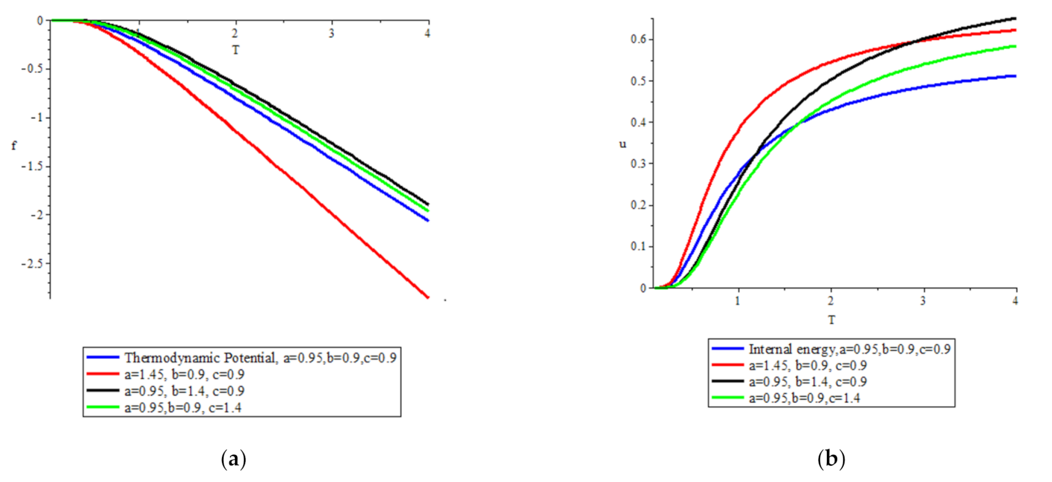
5. Results on the Plasma State

From the thermodynamic potential per magnetic charge of Equation (9), we can determine all the physical magnitudes that can describe the thermal evolution of the magnetic structure of the magnetic monopole gas. This quasiparticle magnetic liquid can have dual similarity with the jellium [51] electronic conductor systems. The magnetic entropy, internal energy, and specific heat are defined as the analytical evolution of thermodynamic functions of the plasma state, as seen in Figure 3. There, we give four values of each physical magnitude for different values of the parameters; although the numerical differences are not great, the variations are clearly manifested in the corresponding plots. In Figure 3a, we find that free magnetic charges begin to appear above 0.4 K, just when the condensate of bosons has already almost completely evaporated. The fermionic thermodynamic potential corresponding to the free charges coming from the broken dipoles only begins to take significant values after these temperatures. In the same way, the internal energy starts to increase, and at lower temperatures, the entropy and the specific heat also increase.

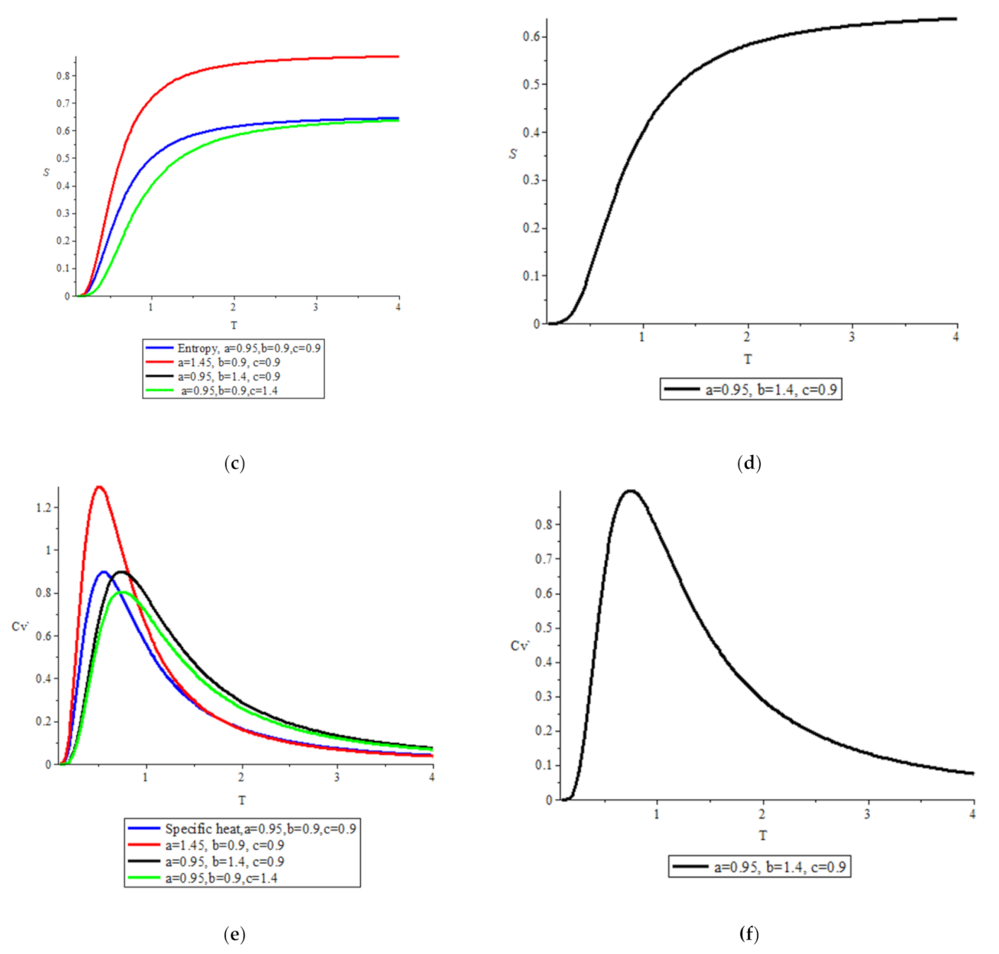
However, this delay is significant in Figure 4, in which it is clear that this separation of the two phases, whose curves of specific heat announce a phase transition from bosonic liquid to fermionic magnetic plasma gas, is evident in the curves of entropy and specific heat.

The different temperature values for the appearance of the maximums of the specific heat fundamentally depend on the expression $\mathbf{exp}\left(-\frac{{\mathsf{\sum }}_{\mathbf{0}}-\mathsf{\mu }}{{\mathbf{K}}_{\mathbf{B}}\mathbf{T}}\right)$ and the term corresponding to the kinetic energy, both in Equations (7)–(9). However, the specific heat values in these maximums almost exclusively depends on the term $\mathbf{exp}\left(-\frac{\mathbf{g}{\mathbf{\varphi }}_{\mathbf{0}}}{{\mathbf{K}}_{\mathbf{B}}{\mathbf{T}}_{\mathbf{C}}}\right)$ such as one can see in Figure 3e.

Although it is true that there are three parameters that intervene in the formation of the different plots of the thermodynamic functions of Figure 3, the values of the maximums of Cv depend fundamentally on the a-parameter, and the temperature at which these maximums appear depends on parameters b and c. This latter parameter depends on the kinetic energy. The red line corresponds to the results obtained with variation in 35% of the a-parameter. The larger the a-value, the larger the absolute value of the corresponding thermodynamic functions. The same variation of the other two parameters yields minor effects in these functions. However, the larger the maximum of the specific heat, the larger the density of tetrahedra per volume unity. This implies that the hydrostatic pressure increases this magnetic plasma specific heat.

On the other hand, for values of the parameters a = 0.95, b = 1.40 and c = 0.90, the graph of the entropy reaches the saturation of ln2 at a temperature of 4 K, which is when the specific heat, due to the number of free magnetic charges, decays, tending to zero. The values of the parameters corresponding to the black curve on the analytical formulation of the specific heat seems to yield the best result corresponding to its maximum in the plasma state, which is found at approximately 0.80 K, which are closed to some experimental results [28,29,30,31,32,33]. The results of the plot of entropy in black also are qualitatively coherent with those obtained experimentally.

These results of Figure 4 show that, until 0.40 K, there are practically no free magnetic charges arising from the broken dipoles, which, according to the dumbbell model, are generated via the spin flips. These reversals of the directions of the spins are those that determine the appearance of excited states whose corresponding quasiparticles can be interpreted as magnetic charges. From this temperature, the dipoles increase their dipole moment via the growth of the separation between their magnetic charges. Then, the conversion of dipoles into Dirac strings begins, until these strings are quickly so long that the attractive interaction energy between charges is inferior to the kinetics of the movement of quasi-free charges. This elongation of splitting between charges of the old dipole makes them closer to completely free charges whose evolution of their thermodynamic functions with temperature is such as one can see in the graphs of Figure 4.

6. Final Comments and Some Conclusions

The main characteristic of the analytical model here presented is based on Hamiltonian 1 inserted in a general model with certain similarities both with a fluid of electrons in a jellium phase [51] and with a gas of mesons explained by Witten [36]. In addition, this Hamiltonian was already used in a previously published paper [47]. In this previous paper, a variational analysis is made, proposing a fundamental state wave function that depends on 2N variational parameters. Minimizing the energy of this variational ground state, we determined the energies of the individual components. These states were bosons formed by pole–antipole pairs in a condensate Bose–Einstein global state [41,42,43,44,45,46,47,48,49] and fermions when the aforementioned dipoles are broken, generating free magnetic charges to increase temperature. These free monopoles are susceptible to be accelerated by a magnetic field, similar to the way in which the electrons are accelerated by the electric field [13,14,15,16]. In the case of this new paper, we consider a simple perturbative procedure with the same Hamiltonian being advantageous with respect to the previous one. The advantage is that the analytical expressions of the thermodynamic functions—specific heat, entropy, internal energy by spin-ice compound formula, number of magnetic charges of each sign per lanthanide vertex, and Helmholtz thermodynamic potential—are easier to obtain. Additionally, the results obtained, given in Figure 1, Figure 2, Figure 3 and Figure 4, with the analytical formulas obtained are more controllable, and their qualitative and quantitative coherence with the experimental results seems to be stronger [26,27,28,29,30,31,32,33,34,35].

If, as in the case of previous work [47], we superimpose the results of the fundamental thermodynamic functions, such as entropy and specific heat, we give a clue of the existence of phase transitions. This is what we did, and its result is reflected in Figure 4. In the plots of this Figure 4, we see how the specific heat is zero at temperature 0 K (see Figure 1b, Figure 2b), as it is given in other investigations [26,27,28,29,30,31,32,33,34,35]. This calorific capacity has an abrupt growth in the first hundredths of kelvin above the fundamental state. This is compatible with a phase transition of a bosonic character to which, in a previous paper, we give clues, which allows us to consider it a bosonic condensation which, in our pseudospin model, is a condensed mixture of a coherent collective state of wave s and p. This mixture has been suggested in the theoretical study of [52]. The evolution of the maximums of specific heat that can be seen, and which we have already mentioned in previous sections of this paper in Figure 2, are between 0.05 and 0.15 K, depending on the parameters already defined in Section 2 and Section 3 of this paper.

Although the curve of this thermodynamic function of specific heat is not exactly symmetrical since its decay is exponential, it clearly denotes that the rupture of the bosonic phase with the appearance of the free-charge fermionic phase coexists in a temperature range of 0.20 to 0.45 K. In this coexistence, the Cv corresponding to the boson condensation is rapidly decreasing, and the one corresponding to the plasma state is increasing. This coexistence disappears rapidly when the number of free charges increases. This numerical growth with temperature can be seen in Figure 4. This growth is less abrupt in the plasma state of quasi-free magnetic charges than that which occurs in the bosonic state. The plasma state reaches a maximum specific heat between 0.6 and 1 K, depending on the values of the parameters defined in Section 4. An evolution compatible with that of the specific heat appears in the entropy, as can be seen in Figure 4b, and whose comment and interpretation are obviously similar to those made regarding the specific heat. In this drawing, the entropy per each quasi-free magnetic charge of the magnetic plasma state (i.e., for the fermionic phase) presents the saturation value of ln2, but it does not have perceptible increases until a temperature of 0.3 K, while the entropy of the bosonic condensation increases from 0.02 K and it does not increase further after 0.2 joules/kelvin. The transition between the two states occurs at approximately 0.5 K, when the two curves of entropy intersect in Figure 4b. Therefore, the results of specific heat and entropy are clearly compatible with the existence of two phase transitions, one whose final is a boson condensate and another one when this transitions to a plasma state in a characteristic fluid of magnetic monopoles. This last transition is, in addition to a thermodynamic transition, a quantum transition since it supposes a change in symmetry from integer spin of the individual components the global state to an half-integer spin.

The results given in Figure 4 are relevant of the article. The other three figures are important for knowing the evolution of the different thermodynamic functions with temperature. However, this Figure 4 is, in addition, indicative of the possible phase transitions. The difference in evolution with the temperature reflected in the graphs is due to the different nature of the pseudospin. This is so since this pseudospin is responsible for the entropy and specific heat behaving at low temperatures as they do in these two graphs: great growth at temperatures less than 0.1 K in the case of dipoles (states of integer pseudospin) and no variation in the case of monopoles (states with half-integer pseudospin) in both specific heat and entropy. In addition, while the plasma state provides zero entropy in the interval $0 \le T \le 0.2 \mathsf{K}$, the boson condensate contributes to the entropy of the system practically all the possible because for 0.2 K the entropy reaches almost the asymptotic value of this phase. Being this behavior similar to that empirically detected and evidenced (see for example see the reference [31]) in such a way that we can say that this behavior is a validity test for the pseudospin model.