Article

Efficient Simulations of Propagating Flames and Fire Suppression Optimization Using Adaptive Mesh Refinement

Paul M. Rady Department of Mechanical Engineering, University of Colorado, Boulder, CO 80309, USA
*
Author to whom correspondence should be addressed.
Fluids 2021, 6(9), 323; https://doi.org/10.3390/fluids6090323
Submission received: 25 June 2021 / Revised: 31 August 2021 / Accepted: 1 September 2021 / Published: 8 September 2021

Abstract

:
Fires are complex multi-physics problems that span wide spatial scale ranges. Capturing this complexity in computationally affordable numerical simulations for process studies and “outer-loop” techniques (e.g., optimization and uncertainty quantification) is a fundamental challenge in reacting flow research. Further complications arise for propagating fires where a priori knowledge of the fire spread rate and direction is typically not available. In such cases, static mesh refinement at all possible fire locations is a computationally inefficient approach to bridging the wide range of spatial scales relevant to fire behavior. In the present study, we address this challenge by incorporating adaptive mesh refinement (AMR) in fireFoam, an OpenFOAM solver for simulations of complex fire phenomena involving pyrolyzing solid surfaces. The AMR functionality in the extended solver, called fireDyMFoam, is load balanced, models gas, solid, and liquid phases, and allows us to dynamically track regions of interest, thus avoiding inefficient over-resolution of areas far from a propagating flame. We demonstrate the AMR capability and computational efficiency for fire spread on vertical panels, showing that the AMR solver reproduces results obtained using much larger statically refined meshes, but at a substantially reduced computational cost. We then leverage AMR in an optimization framework for fire suppression based on the open-source Dakota toolkit, which is made more computationally tractable through the use of fireDyMFoam, minimizing a cost function that balances water use and solid-phase mass loss. The extension of fireFoam developed here thus enables the use of higher fidelity simulations in optimization problems for the suppression of fire spread in both built and natural environments.

1. Introduction

Given the potential hazard and cost of experimental studies, particularly at large spatial scales, computational simulations are an attractive approach to studying fire behavior. However, computationally efficient, full-physics simulations that avoid empirical ad hoc models [1] are required to study fire dynamics over widely varying and realistic conditions, as well as to enable the reliable use of “outer-loop” techniques such as optimization (e.g., for mitigation and suppression efforts) and uncertainty quantification (e.g., for risk assessment).
Perhaps the greatest difficulty in performing such high-fidelity simulations is the wide spatio-temporal scale separation characteristic of fire spread problems. Disparate temporal scales, from relatively slow flow advection to fast chemical reactions, are often addressed by assuming infinitely fast chemistry. This mixed-is-burnt assumption can be made because chemical reactions occur on much shorter timescales than the turbulent mixing timescale for non-premixed flames. The eddy dissipation model [2,3] can then be used to relate the combustion timescale to local turbulence timescales. Flamelet models or other mechanism reduction approaches (e.g., at run-time [4,5,6] or a priori [7,8]) can also be used to balance fidelity with computational cost for problems where the mixed-is-burnt assumption is no longer valid.
Relevant spatial scales range from the small-scale structures of solid fuels to the larger scales characteristic of buildings and warehouses. Methods to address temporal scale separation generally increase the minimum computational timestep, either by not resolving the reaction timescale or by making finite-rate chemistry more affordable. However, the minimum spatial length scale is often dictated by geometric constraints, such as the fuel size or local geometry. Although static mesh refinement can be used to address some of this scale separation, such approaches are inadequate in fire spread problems where the region of interest may be rapidly varying and is not known a priori.
In the present study, we use adaptive mesh refinement (AMR) to address the challenge of bridging wide spatial scale separations in simulations of fire spread. Using AMR, grid cells and physical resolution—and, by extension, computational resources—can be concentrated where they are most needed, for example, to track a propagating flame and make optimization and calibration studies (Nyazika et al. [9] provide a review) more tractable. Previously, Lapointe et al. [10] demonstrated the use of AMR with the OpenFOAM solver fireFoam [11] for simulations of turbulent diffusion flames (resulting in a solver called diffusionFireFoam), and here we introduce a new extension of this solver, called fireDyMFoam, that uses AMR to model fire spread over solid pyrolyzing surfaces. The new solver retains the pre-existing fireFoam capability for modeling multiphase flows, enabling the analysis and optimization of liquid-based fire suppression strategies (e.g., involving liquid films and Lagrangian particles) using computationally efficient AMR-based simulations of fire spread.
In the following, we outline the details of fireDyMFoam, including the treatment of gas, solid, and liquid phases, and provide a description of the AMR approach. We then demonstrate the solver for meter-scale vertical fire spread on combustible panels. We show, in particular, that the solver reproduces results from static mesh simulations with the same fine-scale resolution, but at a substantially reduced computational cost. We then leverage these computational savings and use fireDyMFoam inside an optimization loop, driven by the open-source Dakota toolkit for optimization and uncertainty quantification [12], to minimize fire spread on a combustible panel, similar to previous test cases examined using the Fire Dynamics Simulator [13,14,15]. The new solver also includes dynamic load balancing for efficient AMR of fire spread problems. We have made the solver freely available to the fire modeling community at the public GitHub repository https://github.com/clapointe2011/public (accessed on 24 June 2021) for simulations and optimization of a broad range of fire spread problems.
Note that this study outlines many extensions and improvements to fireDyMFoam that are not present in the earlier diffusionFireFoam solver described by Lapointe et al. [10]. Whereas the diffusionFireFoam solver was limited in scope to simulations of gas-phase diffusion flames without pyrolysis, fireDyMFoam can be used to model fire spread over solid pyrolyzing surfaces, as well as model the multi-phase flow commonly found in fire suppression efforts (e.g., sprinklers). Although prior work using diffusionFireFoam [10] also involved extensive testing of the AMR procedure, demonstrating good agreement for first- and second-order statistics between AMR and static simulations of pool fires, in the present study we demonstrate similar agreement for fire spread simulations, which are made more difficult by the transient and non-stationary nature of the flow. Finally, the use of AMR and the addition of dynamic load balancing, which was not present in diffusionFireFoam, have resulted in lower cost simulations that enable “outer-loop” techniques such as optimization and uncertainty quantification. The demonstration of AMR-enabled simulations using fireDyMFoam for the optimization of fire suppression strategies is one of the primary outcomes of the current study.

2. Computational Framework: fireDyMFoam

OpenFOAM is an open-source, finite-volume computational fluid dynamics platform that includes both pre- and postprocessing functionalities, in addition to a wide array of solvers [16]. In the present study, we focus development on OpenFOAM-7 and implement AMR in the fireFoam solver [10,11,17] for computationally efficient simulations of fire spread over solid pyrolyzing surfaces. Designed for simulations of industrial fire problems, fireFoam incorporates gas-, solid-, and liquid-phase regions, in addition to Lagrangian particle modeling capabilities. It has been used previously to study problems ranging from non-reacting buoyant plumes [18,19] and pool fires with static [11,20,21] and dynamic meshes (i.e., using AMR) [10], to larger room-scale fires [22,23], pyrolysis modeling [24,25,26,27,28], and fire suppression [26,29].
Here, we extend the previous AMR solver, called diffusionFireFoam [10], to address multiphase flows and solid fuel pyrolysis. Now including all modeling capabilities present in fireFoam, the new solver presented herein, called fireDyMFoam, also includes dynamic load balancing to further increase computational efficiency. Each of these developments, which are described in more detail in the following sections, enable the optimization framework described in Section 5.

2.1. Physical Treatment of the Gas Phase

The fireFoam solver is typically used to perform large eddy simulations (LES) and this is also the approach that we take with the AMR-enabled solver fireDyMfoam. In the gas phase, three-dimensional (3D) Favre-filtered compressible Navier–Stokes equations and conservation equations for mass, total enthalpy, and species are solved on a single unstructured computational mesh. These equations are given as
ρ t + · ( ρ U ) = S p ( ρ ) + S f ( ρ ) ,
( ρ U ) t + · ( ρ U i U j ) = p rgh + · τ i j + ρ g + S p ( U ) ,
ρ ( h + K ) t + · ρ U ( h + K ) = · α eff ( ρ h ) + p t + Q rxn + Q rad + S p ( h ) + S f ( h ) ,
( ρ Y i ) t + · ( ρ U Y i ) = · α eff ( ρ Y i ) + ρ ω i + S p ( Y i ) + S f ( Y i ) ,
where unity Lewis and turbulent Prandtl numbers are assumed and τ i j represents the viscous stress tensor given by
τ i j = · μ ( U + ( U ) T ) λ ( · U ) I .
In the above equations, ρ is density, U is velocity, p rgh is dynamic pressure, p is pressure (i.e., p = p rgh + ρ g · x + p ref , where p ref is a reference pressure), g is gravitational acceleration, h is specific sensible enthalpy, and K is specific kinetic energy. The transport coefficients μ eff and α eff are the effective (i.e., molecular plus turbulent) viscosity and thermal diffusivity, respectively. In the enthalpy equation, Q rxn and Q rad represent energy sources (or sinks) due to reactions and radiation, respectively, and in the species transport equation Y i is the mass fraction of the i t h species and ω i is the reaction rate for the i t h species. The terms S p ( φ ) and S f ( φ ) denote Lagrangian particle and liquid film source terms, respectively, for the variable φ , and are zero if unused; more detailed descriptions of these terms can be found in Wang et al. [11], Meredith et al. [26], Ren et al. [29], and Meredith et al. [30,31].
Depending on the choice of turbulence closure used to compute μ eff and α eff , sub-grid scale transport equations may also be necessary to close the governing equations. As in the standard version of fireFoam, we use mixture-averaged density and transport properties; the former is computed using the ideal gas law and the latter are temperature-dependent and computed using empirical correlations. Combustion modeling is assumed to be infinitely fast for non-premixed flames, although finite-rate multi-step chemical models can also be used, and governed by an eddy dissipation model. Radiation modeling is accomplished using a finite volume implementation of the discrete ordinate method. For a detailed description of the gas phase physical treatment in fireFoam, we refer the interested reader to Wang et al. [11].

2.2. Physical Treatment of the Solid Phase

In the solid phase, one-dimensional (1D) conservation equations are solved for mass, energy, and species, given as [27,32,33]
ρ s t = R gas ,
( ρ s h s ) t x ( κ s T s ) x = S rad + S rxn + S gas + S flux ,
ρ s Y i , s t = R i .
Here, ρ s and h s are solid-phase density and specific sensible enthalpy, respectively; Y i , s is the mass fraction of solid species i; R i is the reaction rate of the i th solid species; R gas is the corresponding rate of production of pyrolysate; and  κ s is the solid-phase thermal conductivity. Solid-phase energy source terms include an optional in-depth radiative source, S rad ; a reaction source term, S rxn ; a source term to account for mass loss (or, equivalently, gas production) from the solid phase, S gas ; and an optional enthalpy flux-based source term for gas motion within the solid, S flux . These equations are solved on a series of independent, 1D solid meshes using mixture-averaged properties. To account for the transfer of pyrolysate flux from the solid, a mass flux is computed from the solid mass loss rate and is assumed to immediately enter the gaseous region as a known fuel (e.g., methane or propane) [27,32,33]. Additional details of the solid phase modeling are available in Fukumoto et al. [27], Chaos et al. [32], and Vinayak [33].

2.3. Physical Treatment of Liquid Films and Lagrangian Particles

Liquid regions may be introduced at gas-solid interfaces, and are commonly used to “collect” water droplets for suppression modeling. If used, quasi-3D equations for mass, momentum, and energy conservation are solved in the liquid phase [26,29,30,31]. These equations are given by
( ρ f δ ) t + · ( ρ f δ U ) = S ρ f ,
( ρ f δ U ) t + · ( ρ f δ U i U j ) = δ p f + ρ f δ g + S U ,
( ρ f δ h f ) t + · ( ρ δ U h f ) = S h f ,
where the ‖ subscript denotes components tangential to the solid surface; vector terms therefore only have two components. For the film, ρ f is the film density, δ is the film thickness, U is the film velocity, S ρ f are mass source terms (e.g., addition due to coupling with Lagrangian particles, ejection of mass as Lagrangian particles, and phase change), p f is the total film pressure (e.g., sum of local gas-phase, liquid hydrostatic and capillary pressure, and changes due to particle interaction), S U encompasses momentum-based source terms (e.g., viscous stresses and momentum addition or subtraction due to particle coupling), g is the gravity vector, h f is the film sensible enthalpy, and  S h f are source terms in the energy equation (e.g., conductive and radiative heat transfer, phase change, and particle-based energy sources). A detailed description of all potential source terms is available in Meredith et al. [26], and a summary of film modeling as it is commonly used is available in Ren et al. [29]. The equations are solved on a two-dimensional (2D) mesh and the third direction is captured implicitly by the film thickness δ .
If sprinklers are used, a modeling methodology similar to other fireFoam sprinkler-suppression studies (e.g., Ren et al. [29] and FM Global [17]) is adopted such that water particles are only included as a mode of water delivery; heat transfer and phase change are not considered until the water droplets have been transferred to the solid panel surface and incorporated into the film region. Because the droplet mass, composition, and temperature remain constant, they are therefore governed only by a momentum conservation equation given as
m U p t = S U p ,
where m is the particle mass, U p is its velocity, and S U p represents the forces acting on the particle. Fluid–particle coupling is two-way, and particle source terms are treated semi-implicitly.

2.4. Phase Coupling

Gas–solid–liquid phase coupling is treated in a segregated manner; Lagrangian particles are solved first, followed by solution of the liquid, solid, and gas phases (if a phase is not required, its solution is simply skipped). Interactions between each phase are enabled by the various source terms in the transport equations described previously. At phase boundaries, the phases are coupled via mapped boundary conditions for the velocity, temperature, and reacting species. For velocity, the mass flux of pyrolysate in the solid region is matched to a corresponding mass flux of fuel in the gaseous region using either a one-to-one mapping or an energetically-equivalent mapping (e.g., as implemented in FM Global [17]). For temperature, heat transfer is coupled between the solid, liquid, and gaseous regions, and for the fuel, pyrolysate in the solid region is converted to a known fuel in the gaseous region.

2.5. Adaptive Mesh Refinement (AMR)

Previously, we developed an AMR solver for efficient simulations of turbulent diffusion flames, called diffusionFireFoam [10]. In the present work, we have extended the diffusionFireFoam solver to combine the OpenFOAM dynamic meshing functionality described in Jasak and Gosman [34] with the full suite of physical models (e.g., pyrolysis, Lagrangian particle, and surface film modeling) included in fireFoam. The application of AMR is focused here on the gas phase, where the solutions are 3D and the computations are correspondingly more expensive. By contrast, the solid and liquid regions use 1D and 2D meshes, respectively, and are comparatively cheap to solve. To simplify the use of AMR with mapped boundary conditions (which is necessary to couple solid, liquid, and gaseous regions), faces on any coupled boundary and, by extension, the cells containing said faces, are protected from refinement; they are pre-refined to the highest level of AMR that will be used.
The AMR implementation in OpenFOAM takes the form of a single, unstructured mesh, in contrast to block-structured AMR as used, for example, in Zhang et al. [35]. At user-specified intervals, the mesh is updated based on a single refinement field. Cells with field values between lower and upper bounds are marked for refinement and are split in two in each coordinate direction, such that one cell becomes eight cells in 3D. Similarly, values of the field below a cut-off are identified for coarsening, where the reverse process occurs and cells are recombined. Other input parameters include the refinement frequency and a buffer parameter to “insulate” newly added cells (i.e., make the AMR cell addition more conservative).
The mesh update process is summarized by the following steps [10,34]:
  • If the simulation timestep index is a multiple of a user-specified refinement interval, trigger the mesh update.
  • Scan the user-defined refinement field for cells eligible for refinement. Eligible cells are determined by comparing values of the field to lower and upper refinement bounds. If the cell value lies within the refinement bounds, it is marked as a candidate for refinement. Candidates are then scanned and checked for “refineability”, namely, candidates are considered refinable if they are below the max refinement level and if they are hexagonal cells.
  • Refine the selected cells and protect “buffer” cells around the newly refined cells from un-refinement. Map the solution to the new mesh.
  • Scan points in the mesh for un-refinement, comparing point values to an un-refine level; values lower than this level are tagged for recombination. Cells are then recombined and the solution is mapped once more.
We refer to Jasak and Gosman [34] and Lapointe et al. [10] for a more complete description of the AMR process, including verification and validation of the approach in a range of both non-reacting and reacting flow problems.
Previously, we extended the AMR library in Jasak and Gosman [34] to enable refinement and coarsening on an arbitrary number of fields [10]. These fields are scaled at run-time to range between 0 and 1, although un-scaled fields may also be used; refinement bounds are therefore percents of the maximum value (e.g., the top 99.9 % of values at a given time, or lower and upper bounds of 0.001 and 1, respectively). All of these improvements have also been implemented in fireDyMFoam.
Before continuing, it is also prudent to discuss the application of AMR, specifically, within the context of fireFoam simulations. As described previously, fireFoam solves 3D conservation equations only in the gas phase; solid and liquid phases are 1D and 2D, respectively. This is important for two reasons: (i) native AMR functionality is inherently 3D and (ii) phases are coupled with mapped boundary conditions (with an implied one-to-one mapping) at their respective interfaces.
With regard to the first point, we note that the majority of the computational expense can be attributed to the solution of the gas phase, making the inclusion of AMR there a priority. Additionally, the solid and liquid phases use customized versions of “standard” OpenFOAM meshes, making integration of native AMR functionality non-trivial. Although various researchers (e.g., Rettenmaier et al. [36]) have addressed this integration (e.g., by extending the AMR for use with meshes that are not 3D), we note that the current approach retains thin film and solid phases as released (and extensively validated).
Regarding the second point, extensions to support changing meshes at the interface would ideally be accompanied by the use of 3D meshes in the solid and liquid phases. This extension would also incorporate arbitrary mesh interface (AMI) functionality at interfaces; both extensions will involve non-trivial modifications of the liquid- and solid-phase modeling and will be the focus of future work. For the current work, we focus on the use of AMR in the gas phase and make accommodations to facilitate its addition to fireFoam, such as pre-refining phase interfaces (to match the target maximum level of refinement) and protecting the interfaces from further refinement.
This pre-refinement (as well as the AMR itself) may introduce load imbalances for parallel simulations. Notably, we have also implemented run-time load balancing to maintain a balanced distribution of computational load for AMR cases run in parallel. This implementation was inspired by similar functionality used in hyStrath [37], where processor imbalances are assessed at write-time and system calls are used to redistribute the computational mesh. This method is noteworthy because it allows for the use of native OpenFOAM utilities (e.g., reconstructParMesh, reconstructPar, and decomposePar), but requires minimal code modification (mostly at the solver level) and is easily extendable to other solvers.

2.6. Numerical Treatment

In the gas phase, the conservation equations are solved in a segregated manner and coupled using a procedure (i.e., PIMPLE) involving outer SIMPLE iterations and inner PISO correctors [11]. For fireDyMFoam, we have updated the gas phase procedure to solve energy and species conservation inside the PISO corrector loop, similar to implementations in other OpenFOAM solvers [38,39], to decrease computational cost.
Spatial discretization is nominally second-order accurate; total variation diminishing schemes are employed for the divergence of conserved scalar quantities, and a stabilized central difference scheme is used for the velocity convective term to aid stability. Additionally, in the interest of stability, enthalpy gradients are limited. Diffusive terms are unbounded and second-order with limited non-orthogonal corrections. First-order Euler integration is used to march forward in time.
For the solid phase, we again use second-order methods for spatial discretization and first-order Euler integration for temporal integration. First-order integration in time is also used in the liquid phase, if present; spatially, divergence terms are also first-order and diffusive terms are second-order. A global timestep is computed from a user-specified maximum advective Courant number in the gaseous and film regions and maximum diffusion number in the solid region. Temporal sub-cycling is used (often with a lower, particle-specific Courant number) to march Lagrangian particles forward in time.

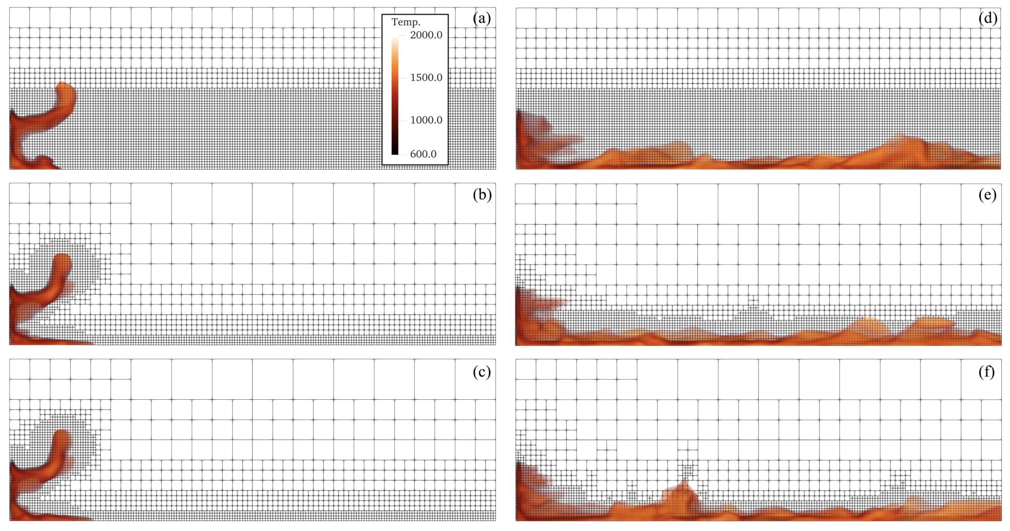
3. Verification: Single Panel Vertical Fire Spread

For the present implementation of AMR in fireDyMFoam to be deemed successful, it must result in a reduction of simulation cost with little or no impact on accuracy, as compared to equivalently refined static mesh simulations. To this end, we first compare the cost and accuracy of AMR in fireDyMFoam against a statically-refined simulation of a vertical fire spread problem (without water droplets or films, for simplicity).
The present case is based on a tutorial included with the standard distribution of OpenFOAM [16], where a [ 0.3 × 0.6 ]  m, 60 kW propane burner is placed in the center of a narrow, initially quiescent domain. The burner is bounded on two sides by [ 0.6 × 2.4 × 0.01 ]  m combustible panels, composed of a homogeneous mixture of unburnt solid cardboard-like fuel and burnt, charred product (set according to the optimized “single-wall” properties in Chaos et al. [40]). The propane burns infinitely fast as it mixes with ambient air, heating the solid, which then pyrolyzes. Combustible products are immediately transferred to the gaseous region, where they are treated as propane and burn infinitely fast, as described below.
For this first demonstration of fireDyMFoam, we focus on a single panel for simplicity, as shown in Figure 1. Static mesh and AMR simulations, described in the following, are performed for this simpler case, and the results are compared to verify that the AMR simulation produces comparable results to the static mesh simulation, but at a lower computational cost.

3.1. Statically Refined Simulation

In the static mesh simulation, a base mesh measuring [ 0.8 × 4.2 × 1.2 ]  m, centered on the propane burner, was created for the solution of the gaseous region with 20 cm resolution. Four nested, static regions of refinement were then created, including a finest refinement region with 1.25  cm resolution occupying a [ 0.4 × 2.5 × 0.8 ]  m volume centered longitudinally on the burner. Figure 2a,d shows slices through the center of the resulting static mesh at z = 0 , indicating the successive regions of static refinement in the x y  plane.
The solid panel region was created by extruding a collection of faces on the boundary of the base mesh, within the 1.25  cm resolution region. An area of size [ 0.6 × 2.4 ]  m was extruded by 1 cm, with 1 mm resolution in the third dimension. The propane burner was created in a [ 0.1 × 0.4 ]  m area on the bottom boundary.
Gas and solid regions were coupled as described in Section 2.6. Within the gas phase, turbulence modeling was accomplished using a one equation eddy-viscosity model with C k = 0.03 [41]. Combustion was modeled using the eddy dissipation method, as implemented in FM Global [17], with coefficients C EDC , C diff , and  C stiff of 4.0 , 0.4 , and  10 10 , respectively [42,43]. Radiation modeling was performed using the finite volume discrete ordinate method with a gray mean absorption-emission model. In the solid phase, model coefficients for thermophysical properties match those from Chaos et al. [40] for the single-layer configuration. Temporal and spatial discretization is set as described in Section 2.6.
As mentioned previously, a custom variant of the PIMPLE algorithm is used [38,39]; one outer PIMPLE iteration (where mass, momentum, and turbulence are solved) and three inner PISO iterations (where species, energy conservation, and pressure correctors are solved) are used to solve the gas-phase conservation equations. A maximum convective Courant number of 0.5 is enforced in the gas phase, and a maximum diffusion number of 0.25 is used for the solid phase; the most limiting constraint is used to compute a single global timestep.
In total, the static mesh for the gaseous region was composed of 449,148 cells and the solid region was composed of 92,160 cells. We ran the simulation in parallel on 6 processors for 15 s of physical time.

3.2. AMR Simulation

The physical configuration of the AMR simulation is identical to that for the static case, described in the previous section and shown in Figure 1. A base mesh of 20 cm is created and the boundary faces along the gas-solid interface and burner are pre-refined by four levels to 1.25  cm resolution, for an initial cell count of 69,048. The solid region is created as before and is therefore identical between the static mesh and AMR simulations.
Within the AMR simulation, four levels of refinement are used in the gaseous region to achieve 1.25  cm resolution, refining on gas-phase heat release rate (HRR) as a measure of combustion strength and location (top 99.9 % of values) and gradients in HRR (top 99.9 % of values) to fully encapsulate regions with combustion. The mesh is updated every four timesteps, and four buffer layers are used. Refinement fields are scaled at run-time to more easily allow assignment of lower and upper refinement bounds. Note that other settings (e.g., other fields and refinement criteria) may give even better results (i.e., further decrease computational cost without affecting simulation accuracy) and the setup used here should be taken as illustrative rather than optimal.
Using the same physical configuration and mesh update procedure, two AMR simulations were performed, corresponding to static and dynamic approaches to grid decomposition and allocation to computational cores. The first AMR case used a time-invariant, geometric decomposition of the gaseous domain, while the second case used run-time load redistribution with the “scotch” decomposition in OpenFOAM. In each case, the decomposition of the solid region did not change with time. For the case with load balancing, mesh redistribution was allowed every 0.1  s of simulation time.

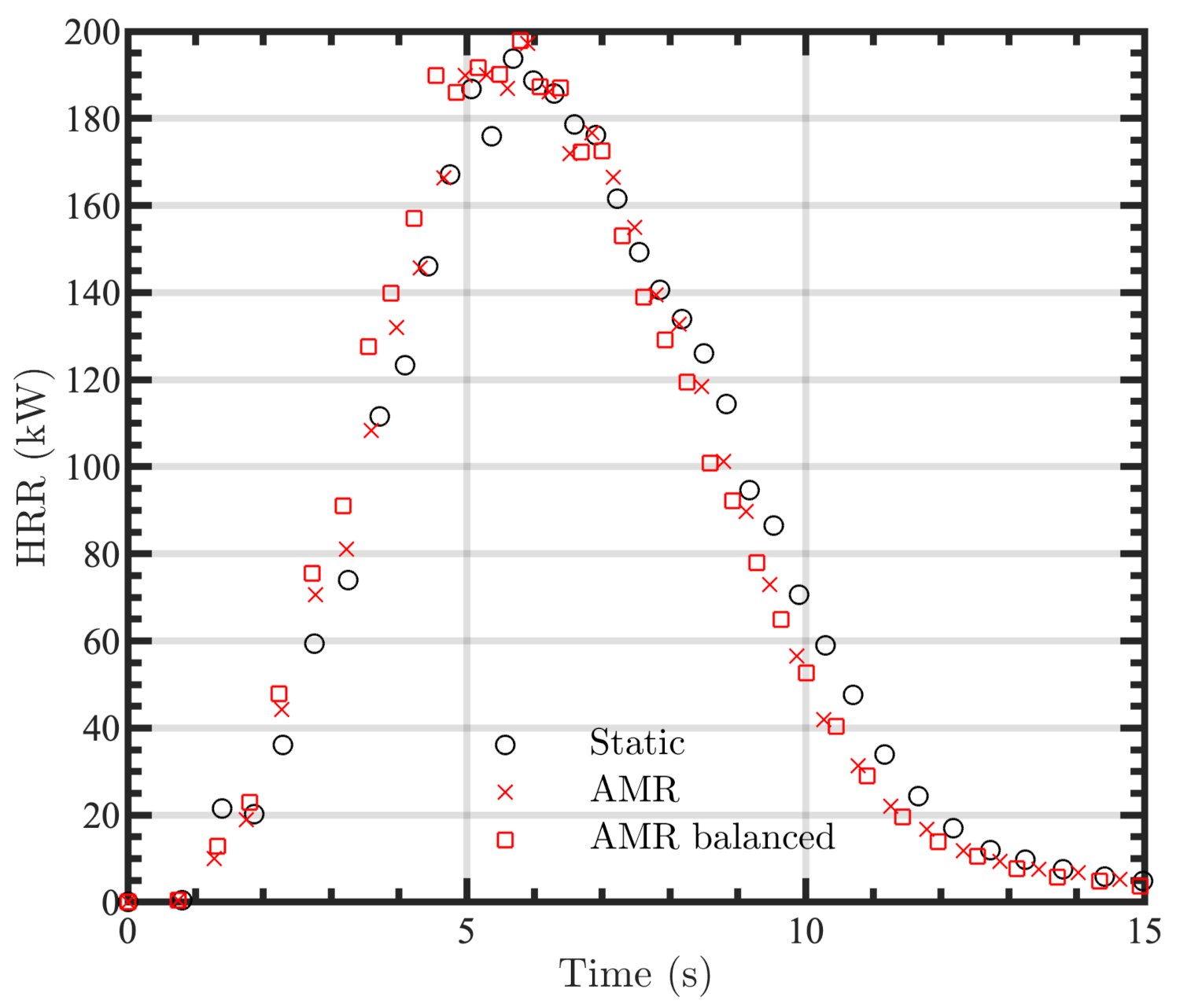
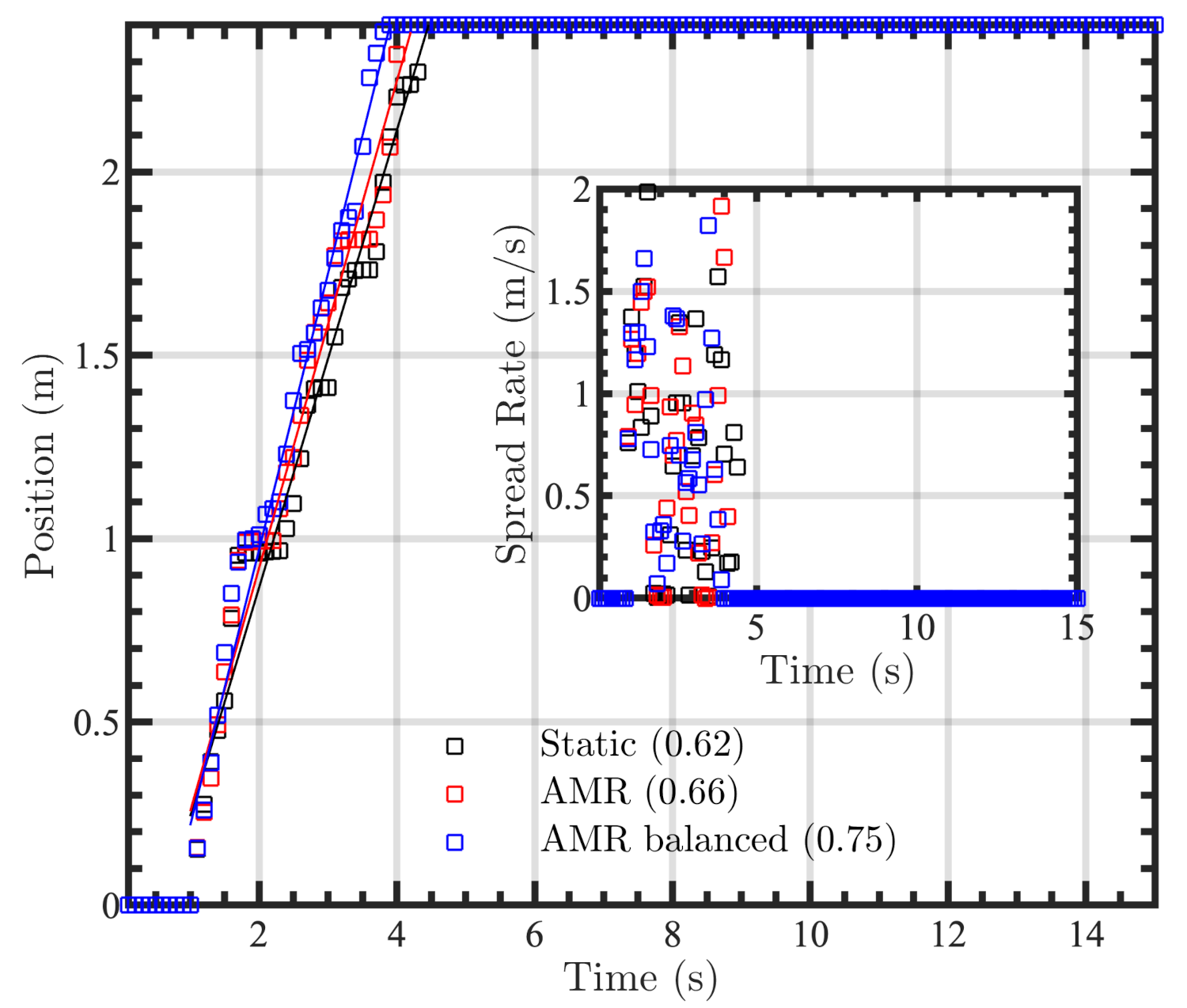
3.3. Results and Discussion

Instantaneous snapshots of regions of high temperature in the gas phase are shown in Figure 2 for the AMR and static simulations at 1.0 and  5.0  s. In general, the hot gases are observed to be qualitatively similar between all three simulations (i.e., the static mesh simulation and the AMR simulations with and without load balancing), with similar gas-phase dynamics between the simulations at both times.
The resulting AMR meshes at 1.0 and  5.0  s are also shown in Figure 2, illustrating the dynamically varying nature of the mesh and the gradually increasing number of grid cells in the AMR cases as the simulation proceeds. The AMR cases started with approximately 69,000 cells in the gaseous region and, once spun up, fluctuated around 130,000 cells (the static mesh simulation had roughly 449,000 cells). The baseline and balanced AMR simulations required an average of 6.0 and 4.6  cpu-hours per physical second of simulation time, respectively, computed as the product of the computation time and the number of cores divided by the physical duration of the simulation (i.e., 15 s). Consequently, we were able to decrease the computational cost relative to the static case, which required an average of 13.6 cpu-hours per second of simulation time. Additionally, we have shown that, although the addition of load balancing makes the simulation even more computationally efficient, both AMR cases were significantly faster than their static counterpart.
From a general quantitative perspective, the time history of chemical HRR, computed as a function of pyrolysate flux into the gaseous region, is compared for the static and AMR simulations in Figure 3, showing good overall agreement. Fire spread, in terms of the distance the flame travels up the panel, is shown in Figure 4, as is the spread rate. This distance is evaluated from char mass fraction slices through the center of the panel at the gas–solid interface. These slices were used to create high-resolution profiles at 0.1  s intervals using Akima interpolation. The furthest location up the panel with char increases of 0.1 % from the initial value for each time was determined for each profile (and thus, each time). The spread rate is quantified in two ways; least squares fits were computed to obtain average rates and instantaneous rates are shown in the inset of Figure 4.
There is generally good agreement between the three simulations in both Figure 3 and Figure 4, and the overall shapes of the time series are quite similar between the three cases. We also note that, although the turbulent nature of these simulations is expected to create local and instantaneous differences in the simulation results, the general correspondence between the AMR and static simulations in Figure 3 suggests that the AMR simulations sufficiently capture the gas phase dynamics necessary for simulations of fire spread. Moreover, the trends apparent in Figure 3 and Figure 4 for the static case are matched by the AMR cases, lending confidence in the use of AMR inside an optimization pipeline where general trends in simulation behavior are expected to be most important.
For a more in-depth comparison, we also investigated the temporal behavior of near-wall temperature (shown in Figure 5), heat flux (Figure 6), and gas-phase modeled HRR (Figure 7) for the static and AMR cases. Examining these figures, we again see good general correspondence between the three cases. This agreement is particularly noteworthy given that no spatial or temporal averaging is used in Figure 5, Figure 6 and Figure 7, and the results in the three figures agree qualitatively and, in many respects, quantitatively, despite the turbulent nature of the simulations.
Note that the computational savings of the AMR simulations are dependent on the choice of refinement fields and their bounds. We have shown here that, for the choices outlined in Section 3.2, the AMR simulations provide results that are comparable to the static mesh results, at a substantially lower computational cost. Additional improvements in efficiency may be achievable for other choices of refinement fields and AMR thresholds, although it should also be noted that further improvements in static mesh simulation cost may also be possible. As such, the present results should be taken as illustrative of the capability of fireDyMFoam, and greater (or lesser) gains may be realized in other problems.

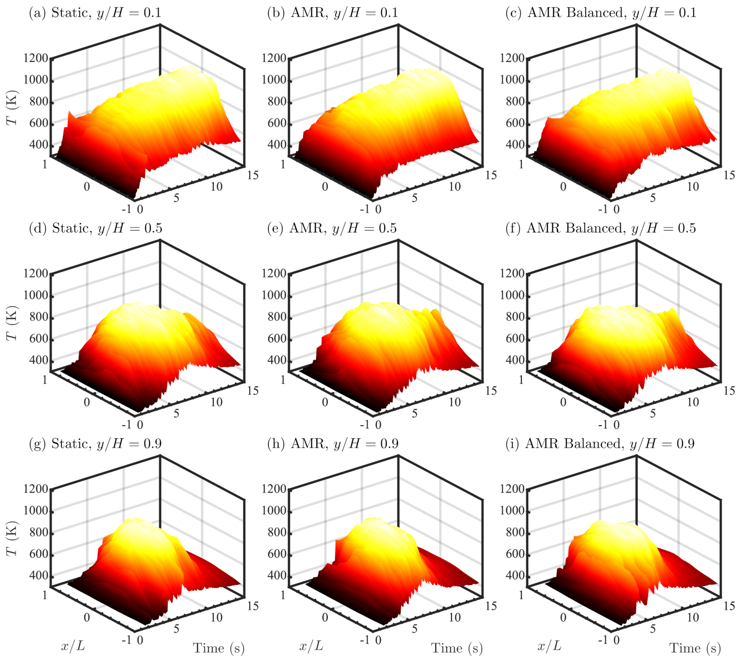
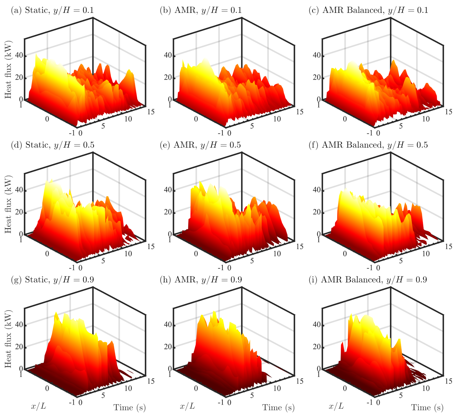
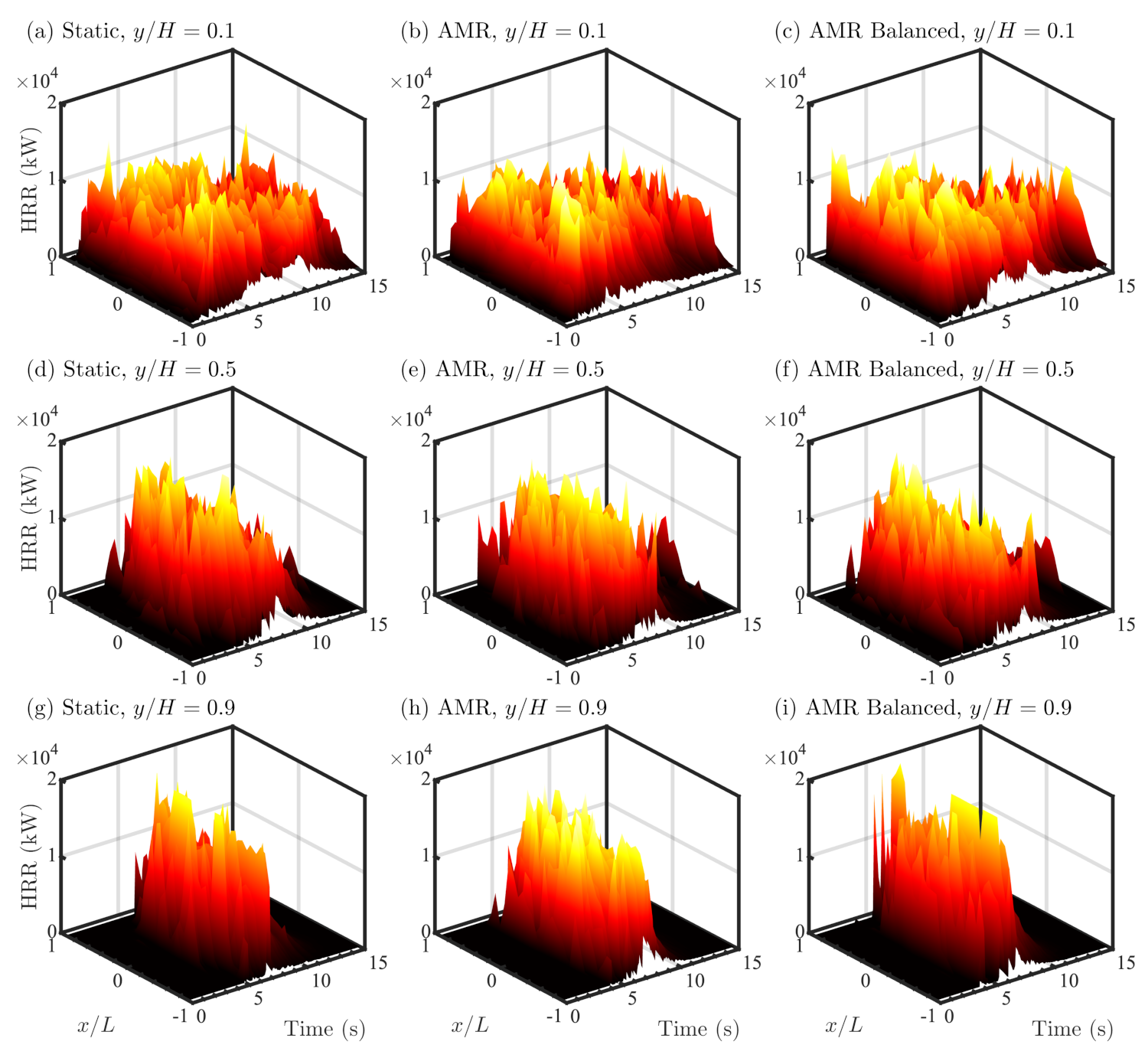
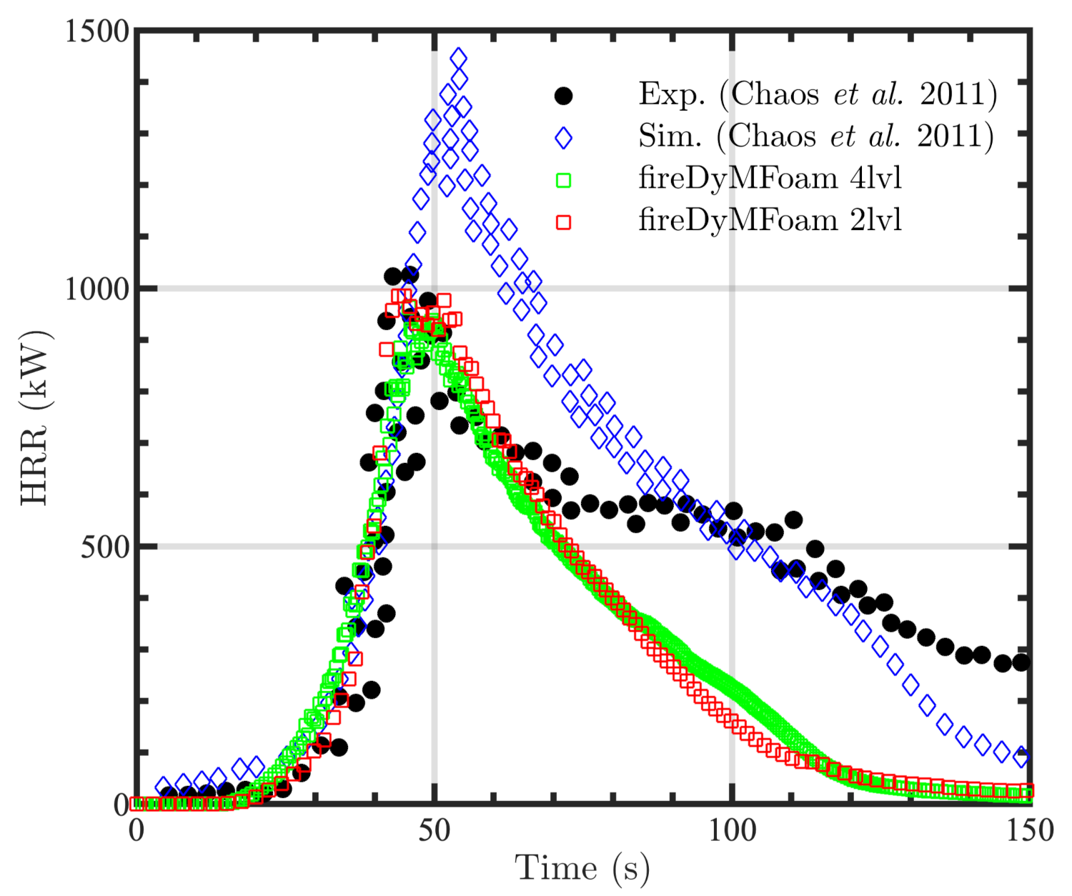
4. Validation: Two-Panel Vertical Fire Spread

Building on the previous single panel vertical spread verification case, we now validate fireDyMFoam against experimental data for a panel spread case similar to the first verification case. In particular, a second panel with identical dimensions, opposite the first, was added to fully replicate the configuration in Chaos et al. [40], where, two [ 0.6 × 2.4 × 0.0154 ] m corrugated cardboard panels are separated by a [ 0.3 × 0.6 ] m 60 kW propane burner. Experimental and computational data for chemical HRR were measured and computed by Chaos et al. [40] for “single-” and “triple-layered” configurations of cardboard, primarily referring to the thickness of each panel, at  3.8  mm and 15.4  mm, respectively. Chaos et al. [40] also completed comprehensive optimization to determine thermophysical settings appropriate for simulating each configuration using the pyrolysis model in OpenFOAM, particularly to match the exponential increase in HRR. Here, we simulate the triple panel configuration and again focus on HRR as a global metric of importance for combustion problems, and only perform AMR simulations.

4.1. AMR Simulation

The physical configuration of the two-panel case largely mimics that of the previous single-panel case shown in Figure 1, but now also includes a second solid region opposite the first. Following Chaos et al. [40], the gas-phase computational domain measures [ 0.3 × 8 × 3 ] m. The first AMR case uses a base resolution of [ 15 × 20 × 15 ] cm and four levels of AMR to achieve an effective resolution of [ 0.94 × 1.25 × 0.94 ] cm to match Chaos et al. [40]. As with the single panel verification case, the mesh boundaries adjacent to the panels on the gas–solid interface are pre-refined and solid regions 15 cells in depth were created for initial gas- and solid-phase cell counts of 65,580 and 368,640 cells, respectively. The case is run in parallel on 16 processors for 150 s.
Based on the recent success by Ren and Wang [44] in simulating a similar case at coarse resolution, we also include a case with base gas-phase resolution of 10 cm using two levels of refinement for a resolution of 2.5  cm. Similar to the four level case, gas–solid interfaces were pre-refined for initial cell counts of 18,456 in the gas phase and 46,080 cells in the solid phase (with the same interface-normal resolution). The case is run in parallel on 3 processors, also for 150 s.
These AMR cases used the same refinement fields and bounds as those used in the single-panel verification case; for each case, the mesh was updated every n flow iterations, where n is the number of refinement levels.
The physical models used in the gas phase are unchanged from the single panel spread verification case. Numerically, the simulations are also largely unchanged; recognizing that these cases must be run out to 150 s, and that general trends in the solution (i.e., HRR) are of primary interest, a maximum Courant number of 0.8 is used to decrease simulation run time. Solid phase thermophysical properties are set based on optimized values reported by Chaos et al. [40], tuned, in particular, to match solid-phase mass loss and mass loss rate, for the “triple-wall” corrugated cardboard; the Arrhenius pre-exponential factor for the solid reaction was adjusted to further improve agreement in each case. The gas and solid phases are coupled as in the previous panel spread case with identical gas-solid interactions.

4.2. Results and Discussion

Once spun up, the AMR simulations had maximum cell counts of roughly 200,000 and 50,000 cells at peak HRR in the four- and two-level simulations, respectively. By comparison, the simulation of Chaos et al. [40] used a static mesh with roughly 600,000 cells (other metrics of computational expense were not reported). Experimental [40] and simulated chemical HRR (computed using the heat of combustion for pyrolysate from Ren et al. [29] and Wang et al. [45]) are compared in Figure 8 for both the static mesh simulation from Chaos et al. [40] and the present AMR simulation using fireDyMFoam.
Quantitatively, Figure 8 shows that the two AMR simulations are in fairly good agreement and provide an accurate prediction of the exponential increase in HRR—the primary goal of these simulations—matching the experimental and computational results from Chaos et al. [40] in terms of the time and rate of increase. As with the reference computational data, the HRR predicted by the AMR cases decays faster than the experimental data. Notably, there is also a marked difference in the peak HRR between the current computational results and those of Chaos et al. [40]. This difference is likely due to the physical modeling used in the simulations, rather than due to the use of AMR itself. We further note that the exact models, namely, the radiation absorption–emission model and solver used by Chaos et al. [40], are not available in OpenFOAM-7, which could help explain the difference in peak simulated HRR. Additionally, carbon oxidation has been identified by Chaos et al. [40] as a possible source of the discrepancies with the experiments, as it is not included in the pyrolysis model. Although extensive model calibration is beyond the scope of the present study, Nyazika et al. [9] have reviewed the utility of such approaches for the case studied by Chaos et al. [40], where char oxidation was also mentioned as a potential source of error.
In the future, this case could be improved, for example, by a more comprehensive tuning of the solid-phase thermophysical properties for use with fireDyMFoam (and, by extension, a newer version of OpenFOAM). This tuning could be completed using the Dakota toolkit as outlined in the following section. In terms of modeling, possible improvements include the incorporation of a char oxidation model in the solid phase (e.g., as implemented by FM Global [17]) and recent developments in wall models for convective heat transfer (e.g., as described by Ren and Wang [44]), updated solid-phase thermophysical parameters (e.g., those used by Ren et al. [29], Ren and Wang [44], and the authors of [45]), and a more in-depth gas phase radiation treatment. As a whole, though, the AMR results shown in Figure 8 are quite encouraging, and the close correspondence between the two- and four-level cases motivates the use of two levels of AMR and 2.5  cm resolution for the optimization cases discussed in the next section.

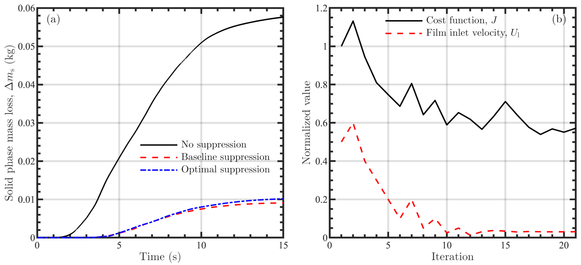
5. Optimization: Fire Suppression Using Liquid Films and Lagrangian Particles

Having shown that AMR simulations using fireDyMFoam are computationally efficient and retain simulation fidelity, notably also at the coarser 2.5  cm resolution, we now leverage the new solver for efficient optimizations of fire suppression methods, where the AMR simulations are coupled to the Dakota open-source toolkit [12] to minimize water use and solid-phase mass loss. For this demonstration, water is either introduced as a film at the top of the panel, or a sprinkler is used to spray water droplets at the panel.
Coupling between Dakota and OpenFOAM is based on similar studies and examples [46,47,48,49,50] and uses a shell script to pass information between the two codes as follows:
  • Retrieve values (e.g., model parameters and boundary coefficients; initial or updated) from Dakota and convert to a format readable by OpenFOAM;
  • Edit OpenFOAM files with values from Dakota;
  • Run OpenFOAM case and post-process as necessary;
  • Compute cost function and pass to Dakota for updated parameter evaluation.
Note that the coupling is quite general and treats the OpenFOAM simulations as a black box. This is beneficial because no modification of the computational software is required. There is a wide array of algorithms included with Dakota, ranging from local algorithms for gradient-based (e.g., Newton and conjugate-gradient methods [51,52]) and gradient-free (e.g., COBYLA [53]) optimization, to global methods such as genetic algorithms [12].

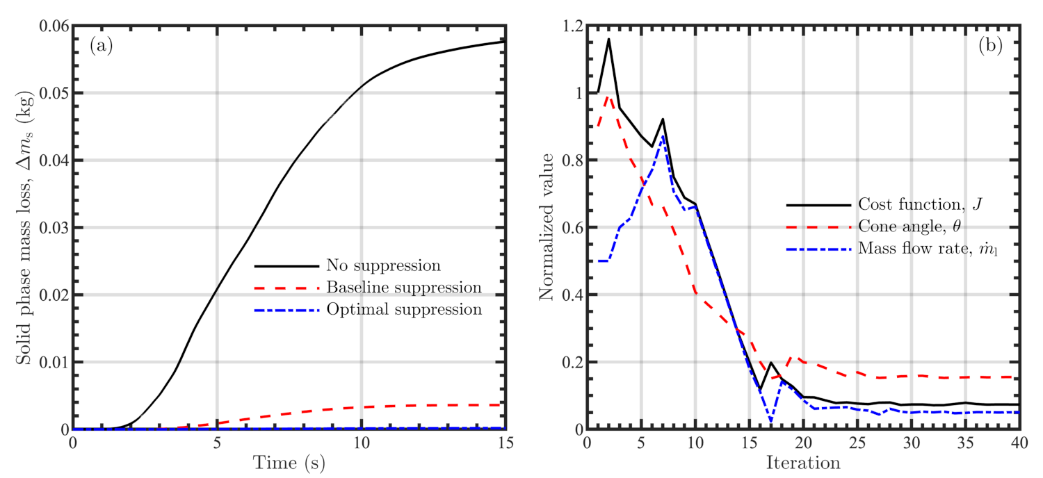
5.1. Water Film Suppression

The first demonstration case focuses on the suppression of vertical fire spread on a single panel via direct application of water. This case is based on the fireFoam tutorial flameSpreadWaterSuppresionPanel, as well as the fire spread simulations described in Section 3 and Section 4. For this case, a liquid water film is introduced at the top of the panel along the gas–solid interface to reduce solid phase mass loss. At the top of the panel, the water has a uniform velocity of 0.01  m/s and a uniform temperature of 298.15  K. The case is otherwise identical in physical configuration to the verification case discussed in Section 3.
Baseline cases with and without the water film were first simulated to demonstrate successful flame suppression. A base mesh with 20 cm resolution was created and boundary faces were refined to 2.5 cm resolution at the gas–solid interface and burner patches. Boundary faces were then extruded to create the solid region, as well as the liquid film region. Three levels of AMR were employed for an effective gas-phase resolution of 2.5 cm in the gas phase. Refinement was based on regions of high HRR and the magnitude of its gradient. The solid and liquid phases were represented using static meshes with identical span-wise resolutions to that used in the gaseous domain. The film region was 1 mm and 1 cell thick, and the solid region was identical to the verification case in Section 3. Each simulation was run for 15 s of physical time.
A comparison of these cases is presented in Figure 9a, where time histories of solid-phase mass loss are compared. Mass loss is used here as a surrogate for the extent of fire spread, where un-suppressed fires are expected to pyrolyze and burn more of the panel, resulting in greater mass loss. In Figure 9a, mass loss is shown to be substantially smaller at all times after roughly 2 s for the case with suppression, as compared to the case without suppression. Most importantly, the large magnitude of this difference suggests that it may be possible to reduce the amount of water introduced while still maintaining a substantially lower cumulative mass loss than the case without suppression.
The challenge of reducing the water flow rate while maintaining adequate flame suppression is ideally suited for optimization techniques. Recognizing that water conservation is important in water-scarce regions of the world, a cost function, J, can be constructed to take both solid-phase mass loss and water use into account as
J = α Δ m s Δ m s ( t = 0 ) + β U l U l ( t = 0 ) ,
where Δ m s is the solid-phase change in mass, U l is the water injection velocity (a measure of water use), and α and β are scaling coefficients set to 0.5 . Both terms in J have been normalized by their respective initial values, with Δ m s ( t = 0 ) obtained from the baseline suppression case and U l ( t = 0 ) = 0.01 m/s. Different values of α and β result in different priorities given to mass loss and water usage during the optimization process, and here we simply set the two coefficients equal for demonstration purposes.
The COBYLA algorithm [53] was used to minimize J subject to 0 U l 0.02 m/s. These bounds were normalized to fall between 0 and 1 as U ^ l = ( U l 0 ) / ( 0.02 0 ) with a normalized starting point of U ^ l = 0.5 . An optimal normalized water velocity of approximately 0.03 , or 6 × 10 4 m/s, was identified in 21 iterations and a plot of the convergence history is shown in Figure 9b.
To demonstrate the success of the optimization, the previous film simulation is updated to use the optimized inflow velocity. The mass loss time history is plotted against the original and baseline histories in Figure 9a, showing that we observe little difference between initial and optimized mass losses while decreasing the water inflow velocity by over an order of magnitude (corresponding to a relatively large amount of water savings), aligning nicely with our expectations for this case.

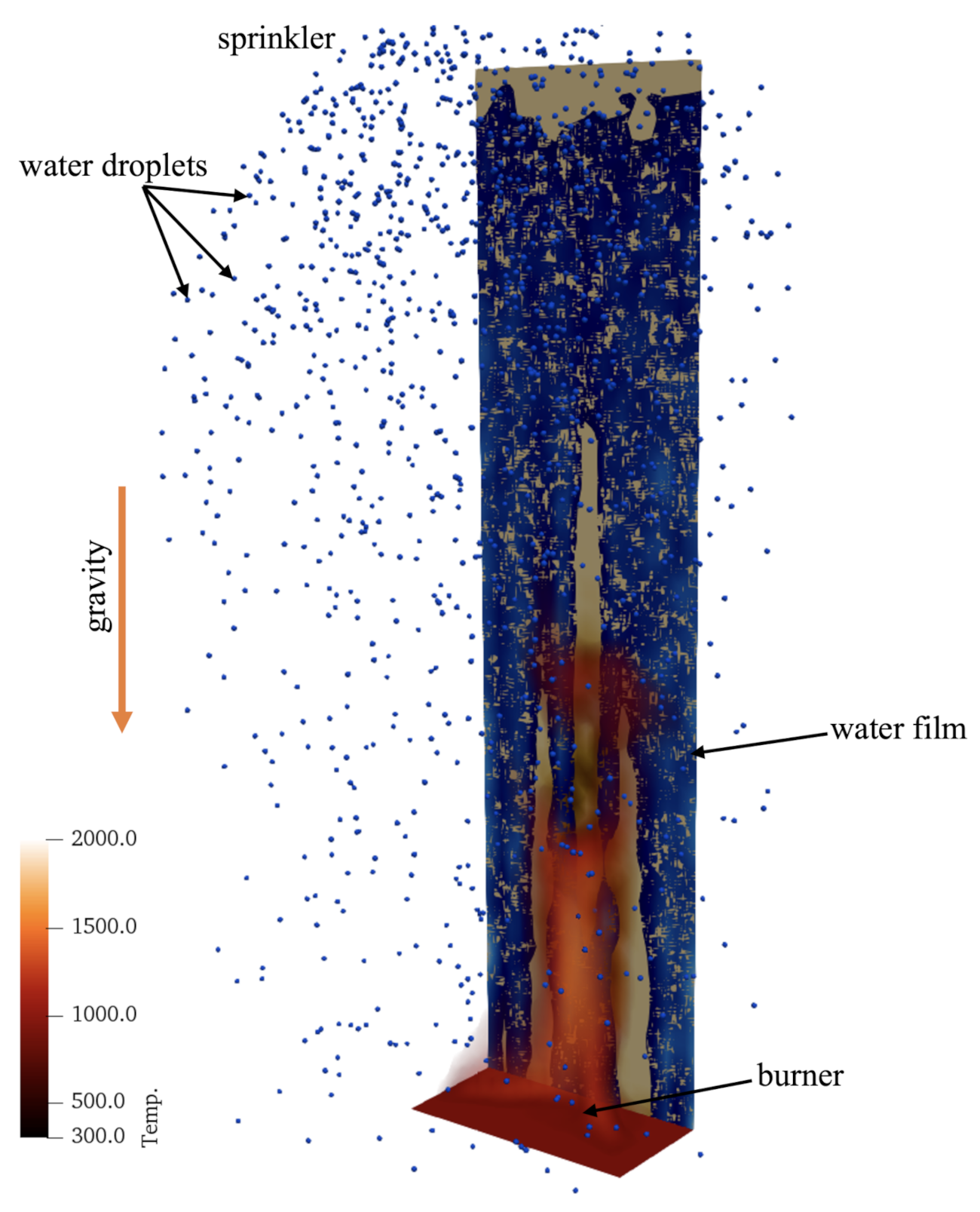
5.2. Sprinkler Suppression

For the second optimization demonstration, a sprinkler is employed as the mode of water delivery. With the addition of Lagrangian particle tracking, this case incorporates all modeling functionality present in fireDyMFoam.
Instead of injecting a steady stream of water at the top of the panel, for this case a collection of water droplets (or “particles”) is sprayed towards the panel at a fixed position, angle, mass flow rate, and temperature. A baseline case, where particles are assumed to have minimal impact on suppression until hitting the solid surface [29,54], with particle settings based on similar tutorial cases (e.g., in The OpenFOAM Foundation [16] and FM Global [17]) is constructed with a sprinkler placed 0.5 m from the panel at a height of 2.4 m that is centered longitudinally. Water is sprayed downwards at an angle 45 below the horizontal towards the panel at a rate of 0.1 kg/s, with a nominal exit speed of 3 m/s and cone angle of 81 . There is two-way fluid–particle coupling and particle source terms are treated semi-implicitly in Equations (1)–(4). Figure 10 shows an annotated 3D rendering of the baseline case, illustrating particles, liquid at the gas–solid interface, the solid, and regions of high temperature in the gas phase.
The baseline case was run for 15 s with the same physical and numerical settings as those used for the water film suppression test case described in Section 5.1 (with the addition of water droplets, as discussed above). Cumulative solid-phase mass loss is compared to the baseline case with suppression in Figure 11a and is observed to be lower than the case without suppression. The baseline case is also visualized in Figure 10, where we observe that some particles miss the panel entirely, suggesting that the injection cone angle as a parameter for optimization; a smaller angle would result in more water hitting the panel, increasing suppression effectiveness (as well as decreasing the volume of water necessary).
Once again, these results indicate that a solid-phase mass loss comparable to that observed in the baseline case may be achievable using less water for a different choice of sprinkler parameters. Here, we again consider a cost function that combines the solid-phase mass loss with total water consumption as
J = α Δ m s Δ m s ( t = 0 ) + β m ˙ l m ˙ l ( t = 0 ) ,
where Δ m s is the solid-phase change in mass, m ˙ l is total liquid mass introduced, and α and β are scaling coefficients set to be 0.5 . Both terms have again been normalized by their respective values from the baseline simulation without suppression and maximum allowable mass introduction, respectively.
The cost function is minimized again using the COBYLA algorithm, varying injected mass flow rate, m ˙ l , and the injection cone angle, θ , subject to the constraints 0 m ˙ l 0.2 kg/s and 0 θ 90 , respectively. The baseline sprinkler case corresponds to a normalized starting point of m ˙ ^ l = 0.5 and θ ^ = 0.9 . In 40 iterations, optimal normalized values of mass flow rate and cone angle were determined to be approximately 0.05 and 0.155 , respectively, corresponding to m ˙ l = 0.01 kg/s and θ = 14 . 0 . Convergence history for this optimization is shown in Figure 11b.
The baseline sprinkler simulation is now updated using the optimized mass and cone angle values, with the time history of solid-phase mass loss shown in Figure 11a. Not only is the optimized solid-phase mass loss lower than the baseline case with suppression, the amount of water necessary was dramatically reduced. In particular, the water mass flow rate is reduced by an order of magnitude compared to the baseline case, which was made possible by reducing the cone angle by a factor of nearly six.

6. Conclusions and Future Work

We have developed a novel extension of the OpenFOAM solver fireFoam that incorporates AMR and retains all multiphase physics originally included with the solver. We have demonstrated that this solver, called fireDyMFoam, provides comparable agreement to static mesh simulations with the same fine-scale resolution for verification and validation cases, at substantially reduced computational cost. Additionally, the verification and validation spread cases were based on existing OpenFOAM tutorials for fireFoam to showcase the easy addition of AMR to fireFoam simulations. Although we primarily highlight the computational benefits of using AMR in this work, we also note that it relaxes hardware requirements; recognizing that simulations using AMR require fewer cells, they can be run on fewer processors (even serial runs are serviceable, as demonstrated by the optimization cases discussed previously).
We then applied fireDyMFoam inside an “outer-loop” optimization process to further demonstrate its potential. The Dakota toolkit was used to drive fireDyMFoam simulations of fire suppression, minimizing a cost function that balanced solid phase mass loss and water use. Although conceptually simple, these demonstrations were successful in finding non-trivial optima and the efficiency gains enabled by the solver will make future large-scale studies more tractable.
There are a number of ways the solver could be improved. In the future, we plan to increase solid modeling capability, for example, by incorporating high-fidelity pyrolysis models in the Porous material Analysis Toolkit (PATO) [55]. As described previously, mapped patches must be pre-refined and protected from further refinement (thereby preventing the solid and liquid meshes from changing size) to enable the use of AMR within the current fireFoam modeling framework. Future work will address this first by adapting the solid solution procedure to be 3D, thus allowing mesh changes similar to the AMR used in the gas-phase throughout this work and making large-scale fire spread problems more computationally tractable. Investigations of AMR use with respect to the liquid phase will then be warranted. Note that the use of Lagrangian particles in the gas phase does not hinder the use of AMR, and other works (e.g., hyStrath [37]) have previously demonstrated such functionality.
Additionally, further investigation of AMR settings (e.g., refinement fields, frequency, and the number of “buffer” layers) would be beneficial as well as the degree of refinement (i.e., the refinement level); noted previously, the chosen settings have been shown to work well but are not necessarily optimal. The coupling with Dakota may also be leveraged for efficient model calibration for fire spread and suppression simulations (similar to, e.g., that used in Nigam [49] and Isaacs et al. [50]). An investigation of temporal, in addition to spatial, adaptivity will also be warranted as problem size increases.
Finally, future research directions also include extensions of the simulations presented in this work, including detailed pyrolysis and soot modeling and larger parameter spaces (e.g., solid fuel properties and more complex suppression configurations like those in Ren et al. [29]) for fire spread and suppression problems.

Author Contributions

Methodology, G.B.R.; Software, C.L., N.T.W., S.S.-W., J.F.G. and P.E.H.; Writing—original draft, C.L.; Writing—review and editing, N.T.W., S.S.-W., J.F.G. and P.E.H. All authors have read and agreed to the published version of the manuscript.

Funding

CL was supported by the NSF Graduate Research Fellowship Program under award DGE 1144083. C.L., N.T.W., S.S.-W., J.F.G., G.B.R., and P.E.H. were supported, in part, by SERDP under grant W912HQ-16-C-0026 and by the 3M Company under project MRA 19-08-0180 TO01.

Data Availability Statement

The fireDyMFoam solver, associated libraries necessary for its compilation (e.g., a custom version of libdynamicFvMesh), and the verification and validation cases can be found at https://github.com/clapointe2011/public/ (accessed on 24 June 2021).

Acknowledgments

The authors would like to thank Yi Wang and Ning Ren of FM Global for their helpful input and for providing experimental data. This work utilized the RMACC Summit supercomputer, which is supported by NSF (awards ACI-1532235 and ACI-1532236), the University of Colorado, Boulder, and Colorado State University.

Conflicts of Interest

The authors declare no conflict of interest. The funders had no role in the design of the study; in the collection, analyses, or interpretation of data; in the writing of the manuscript; or in the decision to publish the results.

References

  1. Hanson, H.; Bradley, M.; Bossert, J.; Linn, R.; Younker, L. The potential and promise of physics-based wildfire simulation. Environ. Sci. Policy 2000, 3, 161–172. [Google Scholar] [CrossRef]
  2. Chen, Z.; Wen, J.; Xu, B.; Dembele, S. Extension of the eddy dissipation concept and smoke point soot model to the LES frame for fire simulations. Fire Saf. J. 2014, 64, 12–26. [Google Scholar] [CrossRef]
  3. Chen, Z.; Wen, J.; Xu, B.; Dembele, S. Large eddy simulation of a medium-scale methanol pool fire using the extended eddy dissipation concept. Int. J. Heat Mass Transf. 2014, 70, 389–408. [Google Scholar] [CrossRef]
  4. Pope, S. Computationally efficient implementation of combustion chemistry using in situ adaptive tabulation. Combust. Theory Model. 1997, 1, 41–63. [Google Scholar] [CrossRef]
  5. Singer, M.; Pope, S.; Najm, H. Operator-splitting with ISAT to model reacting flow with detailed chemistry. Combust. Theory Model. 2006, 10, 199–217. [Google Scholar] [CrossRef]
  6. Singer, M.; Pope, S. Exploiting ISAT to solve the reaction-diffusion equation. Combust. Theory Model. 2004, 8, 361–383. [Google Scholar] [CrossRef] [Green Version]
  7. Niemeyer, K.; Sung, C.; Raju, M. Skeletal mechanism generation for surrogate fuels using directed relation graph with error propagation and sensitivity analysis. Combust. Flame 2010, 157, 1760–1770. [Google Scholar] [CrossRef] [Green Version]
  8. Glusman, J.; Niemeyer, K.; Makowiecki, A.; Wimer, N.; Lapointe, C.; Rieker, G.; Hamlington, P.; Daily, J. Reduced Gas-Phase Kinetic Models for Burning of Douglas Fir. Front. Mech. Eng. 2019, 5, 40. [Google Scholar] [CrossRef]
  9. Nyazika, T.; Jimenez, M.; Samyn, F.; Bourbigot, S. Pyrolysis modeling, sensitivity analysis, and optimization techniques for combustible materials: A review. J. Fire Sci. 2019, 37, 377–433. [Google Scholar] [CrossRef]
  10. Lapointe, C.; Wimer, N.; Glusman, J.; Makowiecki, A.; Daily, J.; Rieker, G.; Hamlington, P. Efficient simulation of turbulent diffusion flames in OpenFOAM using adaptive mesh refinement. Fire Saf. J. 2020, 111, 102934. [Google Scholar] [CrossRef]
  11. Wang, Y.; Chatterjee, P.; de Ris, J. Large eddy simulation of fire plumes. Proc. Combust. Inst. 2011, 33, 2473–2480. [Google Scholar] [CrossRef]
  12. Adams, B.; Bohnhoff, W.; Dalbey, K.; Eddy, J.; Eldred, M.; Gay, D.; Haskell, K.; Hough, P.; Swiler, L. DAKOTA, a multilevel parallel object-oriented framework for design optimization, parameter estimation, uncertainty quantification, and sensitivity analysis: Version 5.0 user’s manual. In Sandia National Laboratories, Tech. Rep. SAND2010-2183; Sandia National Laboratories: Livermore, CA, USA, 2009. [Google Scholar]
  13. McGrattan, K.; Hostikka, S.; McDermott, R.; Floyd, J.; Weinschenk, C.; Overholt, K. Fire dynamics simulator user’s guide. NIST spe Fire Dynamics Simulator User’s Guide. NIST Spec. Publ. 2013, 1019, 1–339. [Google Scholar]
  14. Lee, J. Numerical analysis on the rapid fire suppression using a water mist nozzle in a fire compartment with a door opening. Nucl. Eng. Technol. 2019, 51, 410–423. [Google Scholar] [CrossRef]
  15. Wang, Z.; Wang, W.; Wang, Q. Optimization of water mist droplet size by using CFD modeling for fire suppressions. J. Loss Prev. Process Ind. 2016, 44, 626–632. [Google Scholar] [CrossRef]
  16. The OpenFOAM Foundation. OpenFOAM Development Repository; Github: San Francisco, CA, USA, 2021. [Google Scholar]
  17. FM Global. FireFOAM Development Repository; Github: San Francisco, CA, USA, 2020. [Google Scholar]
  18. Maragkos, G.; Rauwoens, P.; Merci, B. Application of FDS and FireFOAM in Large Eddy Simulations of a Turbulent Buoyant Helium Plume. Combust. Sci. Technol. 2012, 184, 1108–1120. [Google Scholar] [CrossRef] [Green Version]
  19. Maragkos, G.; Rauwoens, P.; Wang, Y.; Merci, B. Large eddy simulations of the flow in the near-field region of a turbulent buoyant helium plume. Flow, Turbul. Combust. 2013, 90, 511–543. [Google Scholar] [CrossRef]
  20. Maragkos, G.; Merci, B. Large Eddy simulations of CH4 fire plumes. Flow, Turbul. Combust. 2017, 99, 239–278. [Google Scholar] [CrossRef] [Green Version]
  21. Maragkos, G.; Beji, T.; Merci, B. Implementation and Evaluation of the Dynamic Smagorinsky Model and an Eddy Dissipation Model with Multiple Reaction Time Scales in FireFOAM. In Proceedings of the 10th Mediterranean Combustion Symposium, Naples, Italy, 17–21 September 2017. [Google Scholar]
  22. Vilfayeau, S.; Ren, N.; Wang, Y.; Trouvé, A. Numerical simulation of under-ventilated liquid-fueled compartment fires with flame extinction and thermally-driven fuel evaporation. Proc. Combust. Inst. 2015, 35, 2563–2571. [Google Scholar] [CrossRef]
  23. Salmon, F.; Lacanette, D.; Mindeguia, J.; Sirieix, C.; Ferrier, C.; Leblanc, J. FireFOAM simulation of a localised fire in a gallery. J. Phys. Conf. Ser. 2018, 1107, 042017. [Google Scholar] [CrossRef]
  24. Ding, Y.; Wang, C.; Lu, S. Modeling the pyrolysis of wet wood using FireFOAM. Energy Convers. Manag. 2015, 98, 500–506. [Google Scholar] [CrossRef]
  25. Ding, Y.; Wang, C.; Lu, S. Large Eddy Simulation of Fire Spread. Procedia Eng. 2014, 71, 537–543. [Google Scholar] [CrossRef] [Green Version]
  26. Meredith, K.; de Vries, J.; Wang, Y.; Xin, Y. A comprehensive model for simulating the interaction of water with solid surfaces in fire suppression environments. Proc. Combust. Inst. 2013, 34, 2719–2726. [Google Scholar] [CrossRef]
  27. Fukumoto, K.; Wang, C.; Wen, J. Large eddy simulation of upward flame spread on PMMA walls with a fully coupled fluid-solid approach. Combust. Flame 2018, 190, 365–387. [Google Scholar] [CrossRef] [Green Version]
  28. Trouvé, A.; Wang, Y. Large eddy simulation of compartment fires. Int. J. Comput. Fluid Dyn. 2010, 24, 449–466. [Google Scholar] [CrossRef]
  29. Ren, N.; de Vries, J.; Zhou, X.; Chaos, M.; Meredith, K.; Wang, Y. Large-scale fire suppression modeling of corrugated cardboard boxes on wood pallets in rack-storage configurations. Fire Saf. J. 2017, 91, 695–704. [Google Scholar] [CrossRef]
  30. Meredith, K.; Xin, Y.; de Vries, J. A numerical model for simulation of thin-film water transport over solid fuel surfaces. Fire Saf. Sci. 2011, 10, 415–428. [Google Scholar] [CrossRef]
  31. Meredith, K.; Heather, A.; De Vries, J.; Xin, Y. A numerical model for partially-wetted flow of thin liquid films. Comput. Methods Multiph. Flow VI 2011, 70, 239. [Google Scholar]
  32. Chaos, M.; Khan, M.; Krishnamoorthy, N.; de Ris, J.; Dorofeev, S. Evaluation of optimization schemes and determination of solid fuel properties for CFD fire models using bench-scale pyrolysis tests. Proc. Combust. Inst. 2011, 33, 2599–2606. [Google Scholar] [CrossRef]
  33. Vinayak, A. Mathematical Modeling & Simulation of Pyrolysis & Flame Spread in OpenFOAM. Master’s Thesis, Bergische Universität Wuppertal, Wuppertal, Germany, October 2017. [Google Scholar]
  34. Jasak, H.; Gosman, A.D. Automatic Resolution Control for the Finite-Volume Method, Part 2: Adaptive Mesh Refinement and Coarsening. Numer. Heat Transf. Part B Fundam. 2000, 38, 257–271. [Google Scholar]
  35. Zhang, W.; Almgren, A.; Beckner, V.; Bell, J.; Blaschke, J.; Chan, C.; Day, M.; Friesen, B.; Gott, K.; Graves, D.; et al. AMReX: A framework for block-structured adaptive mesh refinement. J. Open Source Softw. 2019, 4, 1370. [Google Scholar] [CrossRef]
  36. Rettenmaier, D.; Deising, D.; Ouedraogo, Y.; Gjonaj, E.; De Gersem, H.; Bothe, D.; Tropea, C.; Marschall, H. Load balanced 2D and 3D adaptive mesh refinement in OpenFOAM. SoftwareX 2019, 10, 100317. [Google Scholar] [CrossRef]
  37. Github. hyStrath Repository; Github: San Francisco, CA, USA, 2021. [Google Scholar]
  38. The National Renewable Energy Lab. Simulator for Wind Farm Applications (SOWFA) Repository; Github: San Francisco, CA, USA, 2021. [Google Scholar]
  39. UniCFD Web-Laboratory. Hybrid Central Solvers Repository; Github: San Francisco, CA, USA, 2021. [Google Scholar]
  40. Chaos, M.; Khan, M.; Krishnamoorthy, N.; Chatterjee, P.; Wang, Y.; Dorofeev, S. Experiments and modeling of single-and triple-wall corrugated cardboard: Effective material properties and fire behavior. In Proceedings of the Fire and Materials 2011, 12th International Conference and Exhibition, San Francisco, CA, USA, 31 January–2 February 2011; pp. 625–636. [Google Scholar]
  41. Yoshizawa, A. Statistical theory for compressible turbulent shear flows, with the application to subgrid modeling. Phys. Fluids 1986, 29, 2152–2164. [Google Scholar] [CrossRef]
  42. Vilfayeau, S. Large Eddy Simulation of Fire Extinction Phenomena. Ph.D. Thesis, University of Maryland, College Park, MD, USA, 2015. [Google Scholar]
  43. Ren, N.; Wang, Y.; Vilfayeau, S.; Trouvé, A. Large eddy simulation of turbulent vertical wall fires supplied with gaseous fuel through porous burners. Combust. Flame 2016, 169, 194–208. [Google Scholar] [CrossRef]
  44. Ren, N.; Wang, Y. A convective heat transfer model for LES fire modeling. Proc. Combust. Inst. 2020, 38, 4535–4542. [Google Scholar] [CrossRef]
  45. Wang, Y.; Meredith, K.; Zhou, X.; Chatterjee, P.; Xin, Y.; Chaos, M.; Ren, N.; Dorofeev, S. Numerical simulation of sprinkler suppression of rack storage fires. Fire Saf. Sci. 2014, 11, 1170–1183. [Google Scholar] [CrossRef]
  46. Jareteg, A. Coupling of Dakota and OpenFOAM for automatic parameterized optimization. In Proceedings of CFD with OpenSource Software 2013; Nilsson, H., Ed.; Gothenburg, Sweden, September 2013; Available online: http://www.tfd.chalmers.se/~hani/kurser/OS_CFD_2013/AdamJareteg/report_opensource_AJ.pdf (accessed on 24 June 2021).
  47. Holzmann, T. DAKOTA—OpenFOAM Coupling Training Cases: Geometric Variation. Available online: https://holzmann-cfd.com/community/training-cases/geometric-variation (accessed on 24 June 2021).
  48. Gurreroo, J. Design of experiments, space exploration, and numerical optimization using Dakota and OpenFOAM. In Proceedings of the 11th OpenFOAM Workshop, Vila Flor, Portugal, 26–30 June 2016. [Google Scholar]
  49. Nigam, S. Large Eddy Simulations of Industrial Burners. Master’s Thesis, University of Colorado, Boulder, CO, USA, 2018. [Google Scholar]
  50. Isaacs, S.; Lapointe, C.; Hamlington, P. Development and Application of a Thin Flat Heat Pipe Design Optimization Tool for Small Satellite Systems. J. Electron. Packag. 2020, 143, 011010. [Google Scholar] [CrossRef]
  51. Fletcher, R.; Reeves, C.M. Function minimization by conjugate gradients. Comput. J. 1964, 7, 149–154. [Google Scholar] [CrossRef] [Green Version]
  52. Fletcher, R. A new approach to variable metric algorithms. Comput. J. 1970, 13, 317–322. [Google Scholar] [CrossRef] [Green Version]
  53. Powell, M. A direct search optimization method that models the objective and constraint functions by linear interpolation. In Advances in Optimization and Numerical Analysis; Springer: Berlin/Heidelberg, Germany, 1994; pp. 51–67. [Google Scholar]
  54. Grant, G.; Brenton, J.; Drysdale, D. Fire suppression by water sprays. Prog. Energy Combust. Sci. 2000, 26, 79–130. [Google Scholar] [CrossRef]
  55. Lachaud, J.; Scoggins, J.; Magin, T.; Meyer, M.; Mansour, N. A generic local thermal equilibrium model for porous reactive materials submitted to high temperatures. Int. J. Heat Mass Transf. 2017, 108, 1406–1417. [Google Scholar] [CrossRef]
Figure 1. Schematic of the vertical fire spread case, showing the propane burner in orange, as well as both the panel and gas regions. The orange arrow indicates the direction of gravity.
Fluids 06 00323 g001
Figure 2. Visualization of static, AMR, and balanced AMR verification cases. The gas phase is visualized using volume renders of regions with high HRR for static (a,d), for AMR without load balancing (b,e), and AMR with load balancing (c,f) vertical panel spread cases at times 1.0 s (a–c) and 5.0 s (d–f). Regions are colored by temperature from low (black) to high (yellow). The computational meshes are visualized in a plane through the center of the domain in each panel.
Fluids 06 00323 g002
Figure 3. Comparison of chemical HRR time histories for the single panel vertical fire spread verification test case in the static (black circles), AMR without load balancing (red crosses), and AMR with load balancing (red squares) simulations. HRR is computed from instantaneous mass loss rates from the solid.
Fluids 06 00323 g003
Figure 4. Comparison of fire spread and spread rate, shown in the inset as well as with least-squares fits, up the panel for the vertical fire spread verification test case in the static (black squares, black line), AMR without load balancing (red squares, red line), and AMR with load balancing (blue squares, blue line) simulations. The numbers in parentheses in the legend indicate the slopes of the least squares fits, giving an estimate of the spread rate in m/s for each case. Spread and spread rate were assessed from changes in char at the gas-solid interface.
Fluids 06 00323 g004
Figure 5. Time histories of gas-phase temperature across the panel, near the gas–solid interface, for the single panel vertical fire spread verification test case. Rows from top to bottom show time histories at panel heights of z / H = 0.1 , 0.5 , and 0.9 , where H = 2.4 m is the total height and columns from left to right correspond to static, AMR, and balanced AMR cases, respectively. Temperatures are colored from low (black) to high (yellow). The transverse location x is normalized by the half panel width L = 0.3 m in all plots.
Fluids 06 00323 g005
Figure 6. Time histories of gas-phase heat flux to the solid across the panel, near the gas–solid interface, for the single panel vertical fire spread verification test case. Rows from top to bottom show time histories at panel heights of z / H = 0.1 , 0.5 , and 0.9 , where H = 2.4 m is the total height and columns from left to right correspond to static, AMR, and balanced AMR cases, respectively. Temperatures are colored from low (black) to high (yellow). The transverse location x is normalized by the half panel width L = 0.3 m in all plots.
Fluids 06 00323 g006
Figure 7. Time histories of gas-phase modeled HRR across the panel, near the gas–solid interface, for the single panel vertical fire spread verification test case. Rows from top to bottom show time histories at panel heights of z / H = 0.1 , 0.5 , and 0.9 , where H = 2.4 m is the total height and columns from left to right correspond to static, AMR, and balanced AMR cases, respectively. Temperatures are colored from low (black) to high (yellow). The transverse location x is normalized by the half panel width L = 0.3 m in all plots.
Fluids 06 00323 g007
Figure 8. Time history of chemical heat release rate (HRR) for the two-panel fire spread validation case. Experimental and simulation results from Chaos et al. [40] are shown as black circles and blue diamonds, respectively, and AMR simulation results from fireDyMFoam using four levels of refinement and two levels of refinement are shown as green and red squares, respectively.
Fluids 06 00323 g008
Figure 9. Solid-phase mass loss comparison for panel fire spread cases with and without water film suppression (a) and convergence history for the optimization (b). Panel (a) shows the mass loss for cases with no suppression (solid black line), baseline suppression parameters (dashed red line), and optimal suppression parameters (dash-dot blue line). Panel (b) shows normalized values of the cost function J from Equation (13) (solid black line) and the film inlet velocity U l (dashed red line).
Fluids 06 00323 g009
Figure 10. Visualization of baseline sprinkler case, showing gas, liquid, and solid phases. Gas-phase combustion is visualized by a volume-render of cells with high temperature colored from low (black) to high (red) and solid-phase pyrolysis is visualized by char production colored low (tan) to high (black). Water is shown in blue for particle- and film-based liquid.
Fluids 06 00323 g010
Figure 11. Solid-phase mass loss comparison for panel fire spread cases with and without water sprinkler suppression (a) and convergence history for the optimization (b). Panel (a) shows the mass loss for cases with no suppression (solid black line), baseline suppression parameters (dashed red line), and optimal suppression parameters (dash-dot blue line). Panel (b) shows normalized values of the cost function J from Equation (14) (solid black line), the cone angle θ (dashed red line), and the mass flow rate m ˙ l (dash-dot blue line).
Fluids 06 00323 g011
Publisher’s Note: MDPI stays neutral with regard to jurisdictional claims in published maps and institutional affiliations.

