Article

Numerical Studies of Disperse Three-Phase Fluid Flows

Department of Mechanical Engineering, Johns Hopkins University, Baltimore, MD 21218, USA
*
Author to whom correspondence should be addressed.
Fluids 2021, 6(9), 317; https://doi.org/10.3390/fluids6090317
Submission received: 29 June 2021 / Revised: 31 August 2021 / Accepted: 2 September 2021 / Published: 6 September 2021

Abstract

:
The dynamics of a three-phase gas–liquid–liquid multiphase system is examined by direct numerical simulations. The system consists of a continuous liquid phase, buoyant gas bubbles, and smaller heavy drops that fall relative to the continuous liquid. The computational domain is fully periodic, and a force equal to the weight of the mixture is added to keep it in place. The governing parameters are selected so that the terminal Reynolds numbers of the bubbles and the drops are moderate; while the effect of bubble deformability is examined by changing its surface tension, the surface tension for the drops is sufficiently high so they do not deform. One bubble in a “unit cell” and eight freely interacting bubbles are examined. The dependency of the slip velocities, the velocity fluctuations, and the distribution of the dispersed phases on the volume fraction of each phase are examined. It is found that while the distribution of drops around a single bubble in a “unit cell” is uneven and depends on its deformability, the distribution of drops around freely interacting bubbles is relatively uniform for the parameters examined in this study.

1. Introduction

The dynamics of a three-phase gas–liquid–liquid multiphase system is examined by direct numerical simulations, where the continuum equations describing fluid flows are solved sufficiently accurately so that every length and time scale are fully resolved for unsteady systems. The system consists of a continuous liquid phase, buoyant gas bubbles that rise, and heavy drops that fall, relative to the continuous liquid. Three-phase gas–liquid–liquid systems are found in many engineering applications. One of the more common ones consists of gas bubbles and oil drops in water as found in, for example, water management in the oil industry and the separation of oil and grease from municipal and industrial wastewater. The density difference between oil and water is generally small, so separation relying on gravity-driven settling is slow. However, by injecting gas bubbles into the mixture that stick to the oil drops and carry them to the top, the rate of separation can be greatly increased. While the collision of bubbles and drops and their subsequent interactions, such as when an oil drop engulfs an air bubble, are critical to the efficiency of the process, here, we focus on the flows where the drops do not stick to the bubbles. Since the sticking adds new physical processes and parameters not included here, we believe that the non-sticking case is an important reference case and one that can also describe the pre-collision stage. For a relatively recent review of gas flotation see [1], and discussions of the capture of an oil drop by a gas bubble can be found in [2,3,4], for example. Oil–water–gas flows are also found in many other circumstances, such as in oil wells and pipelines [5].
Numerical simulations, particularly direct numerical simulations, have come a long way in the last two decades. Early simulations of many interacting bubbles can be found in [6], who examined bubbles in initially quiescent liquid in fully periodic domains, and more recent studies include [7,8] where the dynamics of bubbles in turbulent channel flows is examined. While a large number of authors have examined the dynamics of two-phase flows, fully resolved numerical simulations of three-phase systems are relatively rare and usually concerned with systems different from the one considered here. Those include simulations of bubbles and drops in minichannels using a volume of the fluid method by [9], Ref. [10], who used a level set method to study drops in two-layer stratified flows, and Ref. [11], who examined the dynamics of a drop on the interface between two different fluids, using smooth particle hydrodynamics. The only study we have found of the dynamics of fully resolved bubbles and drops is [12], where a method that is referred to as density functional hydrodynamics was used. Several pictures of the interaction of a few bubbles with a few drops are presented but no quantitative information.
While the focus here is on the interactions of buoyant bubbles with heavy drops, we expect the dynamics before the collision to be similar to the interaction of spherical solid particles with bubbles, such as in froth flotation for mineral processing and recycling of plastics, where hydrophobic particles stick to bubbles and are carried to the top of the mixture and removed [13,14]. Most simulations of such systems involve considerable simplifications such as where the bubbles and the flow around them are fully resolved, but the solid phase is modeled as point particles. Ref. [15] simulated the motion of bubbles in initially quiescent flow using a front tracking method to track the bubble surface but modeling the particles as point particles, with two-way coupling. The bubbles were initially put in the lower part of the computational domain, which contained a large number of particles, and the simulations examined how particles were transported in the wake of the bubbles as they left the particle-rich region. A similar study was conducted by [16], who simulated the motion of one and two bubbles and their interactions with point particles, using a VOF method to represent the bubble. Those studies were, however, limited to two-dimensional flows. Other authors have focused on the interaction of a single bubble with point particles. Those include [17], who captured the bubble by a phase-field method and [18], who used an LBM method. Refs. [19,20] studied the influence of turbulence on the interaction of several point particles with a single bubble but used a k ϵ models for the turbulence, rather than fully resolving the flow. In some cases, the bubbles are also modeled as point particles, such as by [21], who simulated turbulent flow with bubbles and solid particles, both modeled as point particles using a one-way coupling, so the disperse phases did not affect the carrier phase. Similarly, a discrete element method has been used to examine the interaction of several point particles with one bubble in [22,23]. The only simulations that we are aware of, where both the bubbles and the solid particles are resolved, are [24,25], who used a front tracking method for the bubbles and an immersed boundary method (IBM) for the solid particles to simulate the interactions between several bubbles and drops, and [26], who used a volume-of-fluid (VOF) method for the bubbles and examined the interactions of a few bubbles and particles. Modeling of three-phase systems using Euler–Euler models for the average flow are more common. For bubbles and drops see, for example, Ref. [27], and for bubbles and solid particles see the extensive review by [28].

2. Numerical Method and Problem Specification

We consider incompressible flow consisting of different fluids or phases, evolving in time, governed by the Navier–Stokes equations as follows:
ρ u t + · ρ u u = p + ( ρ ρ a v g ) g + · μ ( u + u T ) + f σ and · u = 0 .
Here, u is the velocity, p is the pressure, ρ is the density, μ is the viscosity, g is the gravity acceleration, and f σ is the surface tension term. Solving these equations accurately gives the fully resolved flow field at any given time and spatial location. To identify the different phases, we define two index or marker functions, χ b to identify the gas phase and χ d to identify the heavy droplet phase.
χ b ( x ) = 0 in the liquid 1 in the bubbles , χ d ( x ) = 0 in the liquid 1 in the drops .
The various flow quantities, such as density and viscosity can then be written as
ϕ i = ϕ l + ( ϕ b ϕ l ) χ b + ( ϕ d ϕ l ) χ d
where ϕ l is the property of the continuous liquid, ϕ b is the property of the bubbles, and ϕ d is the drop property. Surface tension is assigned to each interface point and is different for the bubbles and the drops.
The governing equations are solved using an explicit second-order finite volume projection method on a staggered fixed regular grid. The advection terms are approximated by a QUICK upwind scheme and the viscous terms by a centered scheme. To update the marker function, and thus the material properties, we represent the interfaces between different fluids by connected marker points (usually called front) that move with the fluid velocity. The marker function is then constructed from the location of the marker points. Surface tension is computed on the front and transferred to the fixed grid and added to the discrete Navier–Stokes equations. For a detailed description of the method and various verification tests, see [29].
The computational domain is a 3D hexahedron, with periodic boundaries in all directions, and to prevent the system from “falling” due to gravity, we add a positive upwards force equal to the weight of the mixture ( ρ a v g g ).
The dynamics of systems with bubbles or drops is usually described by the Morton and Eötvös numbers, defined by
M = Δ ρ g μ 4 ρ 2 σ 3 E o = Δ ρ g d 2 σ .
For our system, we need to specify those for both the bubbles and the drops. In addition, the volume fraction is generally needed for multiphase systems, and in this study, where we work with bubbles and drops of specific sizes, we report the number of bubbles N b and the number of drops N d .

3. Results

3.1. One 3D Bubble and Several Drops

We start by examining the motion of one relatively large bubble and several randomly placed smaller drops in a cubical computational domain with side lengths equal to 1, resolved by a 64 3 grid. The bubbles have a diameter d b = 0.4 , and the droplets have diameters d d = 0.2 . The density and viscosity of the continuous fluid are ρ l = 1.0 and μ l = 0.002 , respectively; for the bubble, we have ρ b = 0.05 and μ b = 0.0004 , and for the drops ρ d = 2.0 and μ d = 0.016 . Surface tension is σ d = 0.01 for the drop–liquid interface, but the surface tension for the bubble–liquid interface is varied, resulting in different Morton and Eötvös numbers, as shown in Table 1. While the grid resolution is relatively low, grid refinement studies have confirmed that the results are reasonably accurate and correctly describe the dynamics of the system. Similarly, we have taken the density of the bubbles to be only 1/20 of the liquid, since we generally find that taking it smaller has only a minor influence on the dynamics, and systems with small density differences are easier to simulate. The number of drops is varied; we show results for N d = [ 12 , 16 , 20 ] . The simulations were run up to time 200, at which time the bubble had passed about 40 times through the computational domain.
Figure 1 shows the bubble and the 12 drops at time 0 and time 100 for E o b = 2.0 and E o b = 10.0 . For the lower Eötvös number, the bubble deforms only slightly as it rises, but for the higher ones, more deformation is seen. The drops remain essentially spherical. The results for E o b = 0.5 are similar to the E o b = 2.0 case, and the E o b = 5.0 results fall in-between the E o b = 2.0 and the E o b = 10.0 case. In addition to the bubble and the drops, the enstrophy ( E = ω · ω ) is plotted in a plane cutting through the middle of the domain to gain insight into where vorticity is generated and where it ends up. The highest values are ahead and behind the bubble, spanning the region between the bubble in one period and the next, suggesting it is the bubble that produces most of the vorticity and that it remains in its wake.
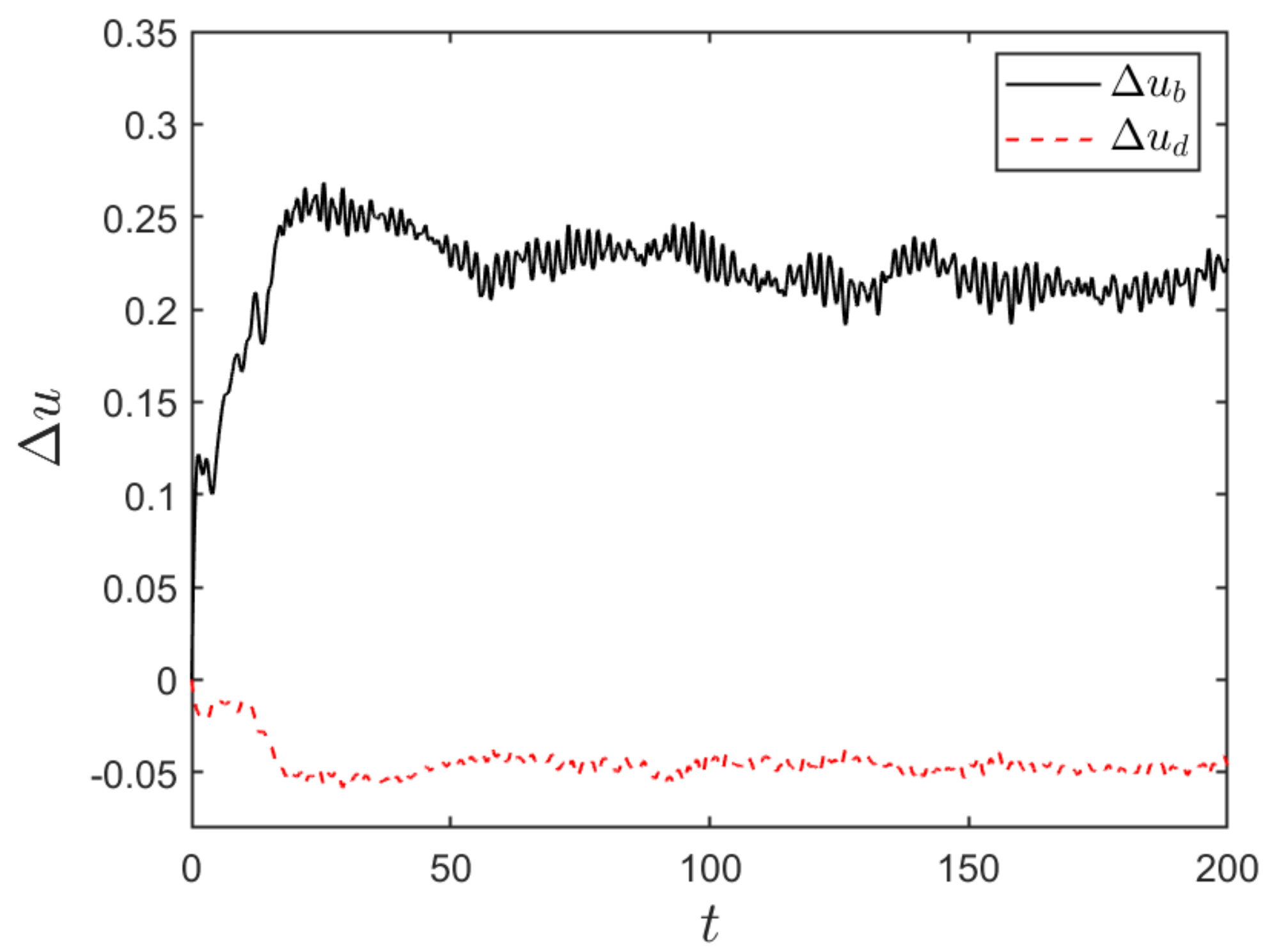
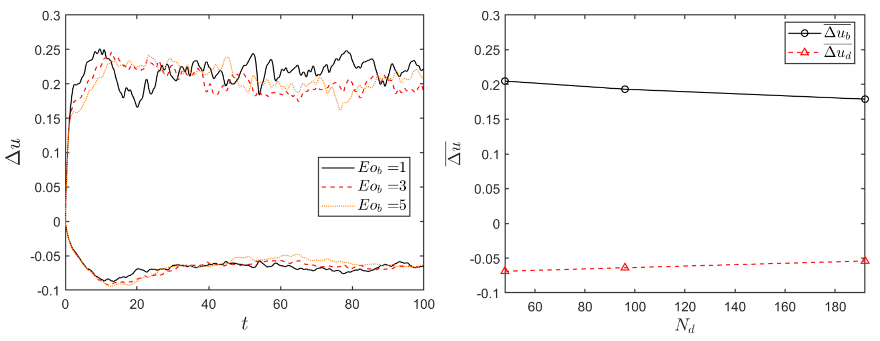
The slip velocities of the bubble and the drops are plotted versus time for E o b = 2.0 and N d = 12 in Figure 2. The bubble wobbles slightly as it rises, as is seen in the nearly periodic oscillations in the slip velocity. For the drops, we plot the average slip velocity, which is negative and relatively steady. After the initial transient, the system reaches an approximately stationary state where the average motion does not change. When we compute average steady-state quantities for the system (shown below), we start at time t = 100 and average until the last time simulated ( t = 200 ). Results for other bubble Eötvös numbers and different numbers of drops are similar.
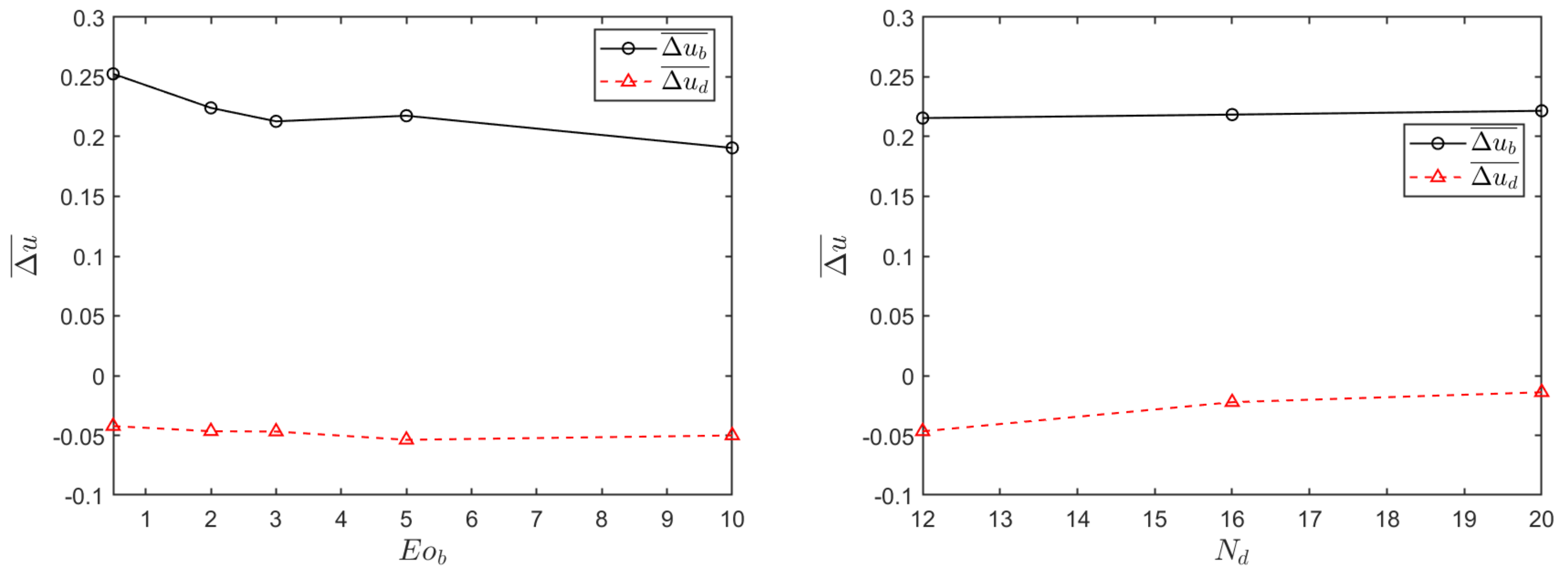
The slip velocity values between the bubble and the continuous liquid, as well as between the heavy drops and the continuous liquid averaged over time after the system reaches an approximate stationary state, are shown in the left frame of Figure 3 versus Eötvös number of the bubble ( E o b ) and N d = 12 . It is clear that while the droplet velocity remains nearly unchanged, the bubble slows down slightly as it becomes more deformable, although the decrease is relatively small and not completely monotonic. The right frame of Figure 3 shows the averaged slip velocity for different numbers of drops for E o b = 2.0 , and while the bubble velocity is only minimally affected, the velocity of the drops decreases slightly as their number is increased.
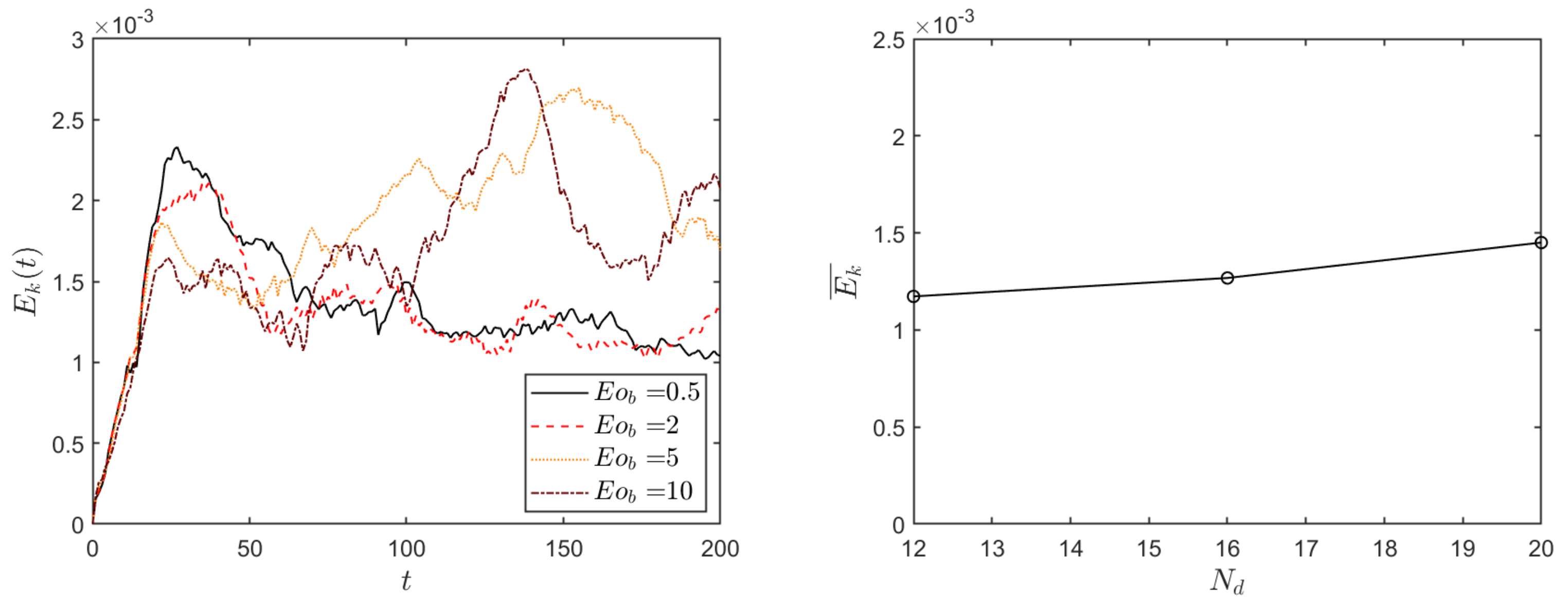
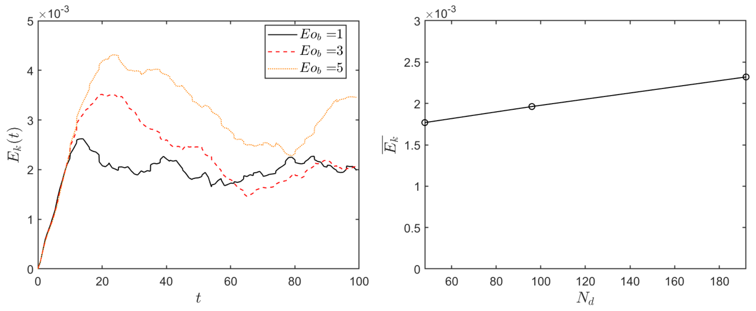
In Figure 4, we examine the velocity fluctuations in the liquid by plotting the kinetic energy of the liquid versus time for four Eötvös numbers on the left and the average kinetic energy versus the number of drops for E o b = 2 on the right. For the less deformable bubbles the kinetic energy is relatively constant after an initial sharp rise, but for the more deformable bubbles, we see large fluctuations at later times. The dependency of the average kinetic energy in the liquid on the number of drops rises slightly with the number of drops, but the dependency is weak. Similar results are seen for other Eötvös numbers.
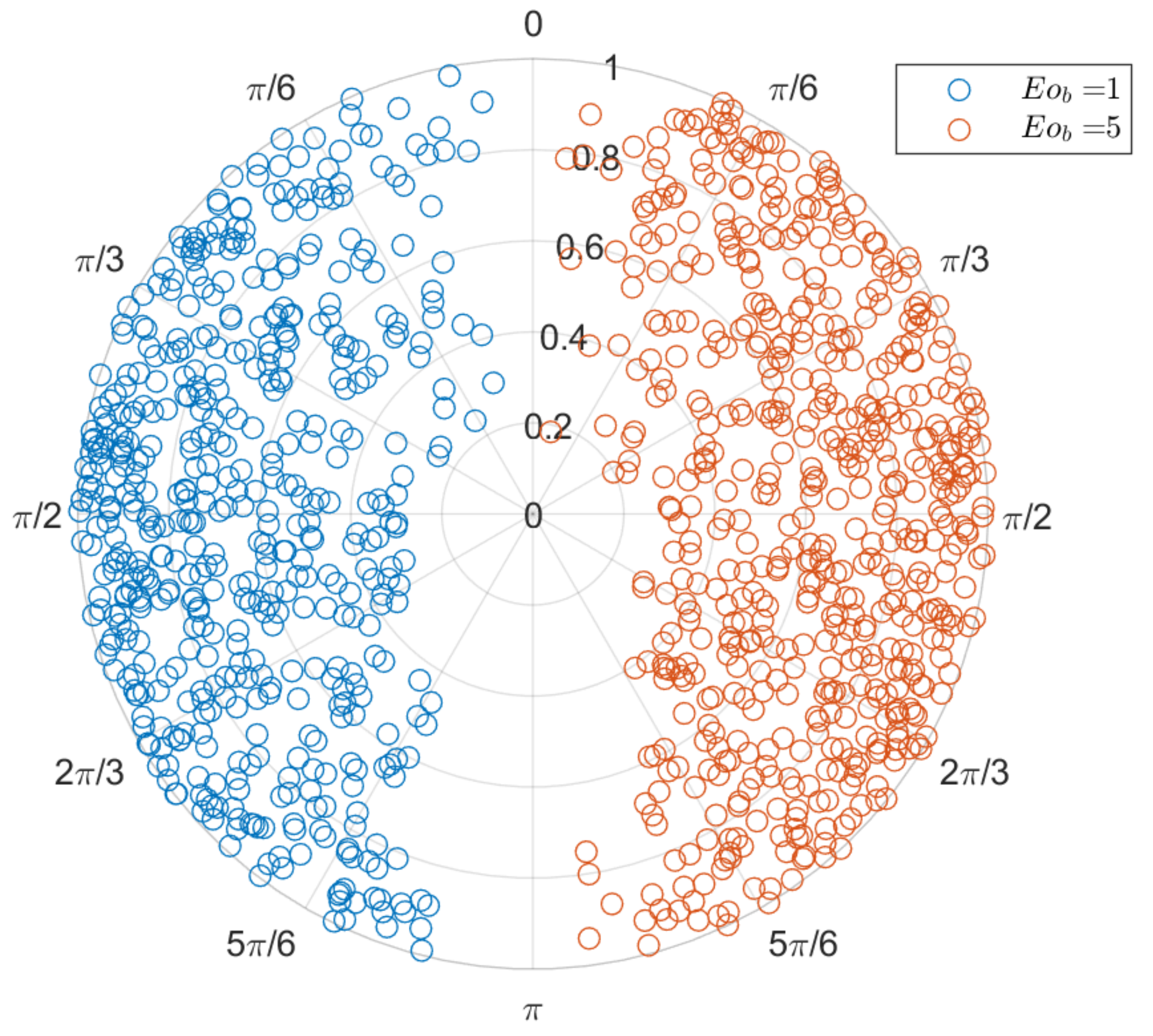
One of the main questions in many applications of dispersed three-phase flows is how the drops (or solids) and the bubbles interact. In wastewater remediation, the efficiency of the process depends critically on the bubbles colliding with and capturing droplets, and the same is true for flotation in mineral processing, where the drops are replaced by solid particles. To examine how the droplets are distributed around the bubble, we show the angular and radial location of droplets with respect to the bubble in 
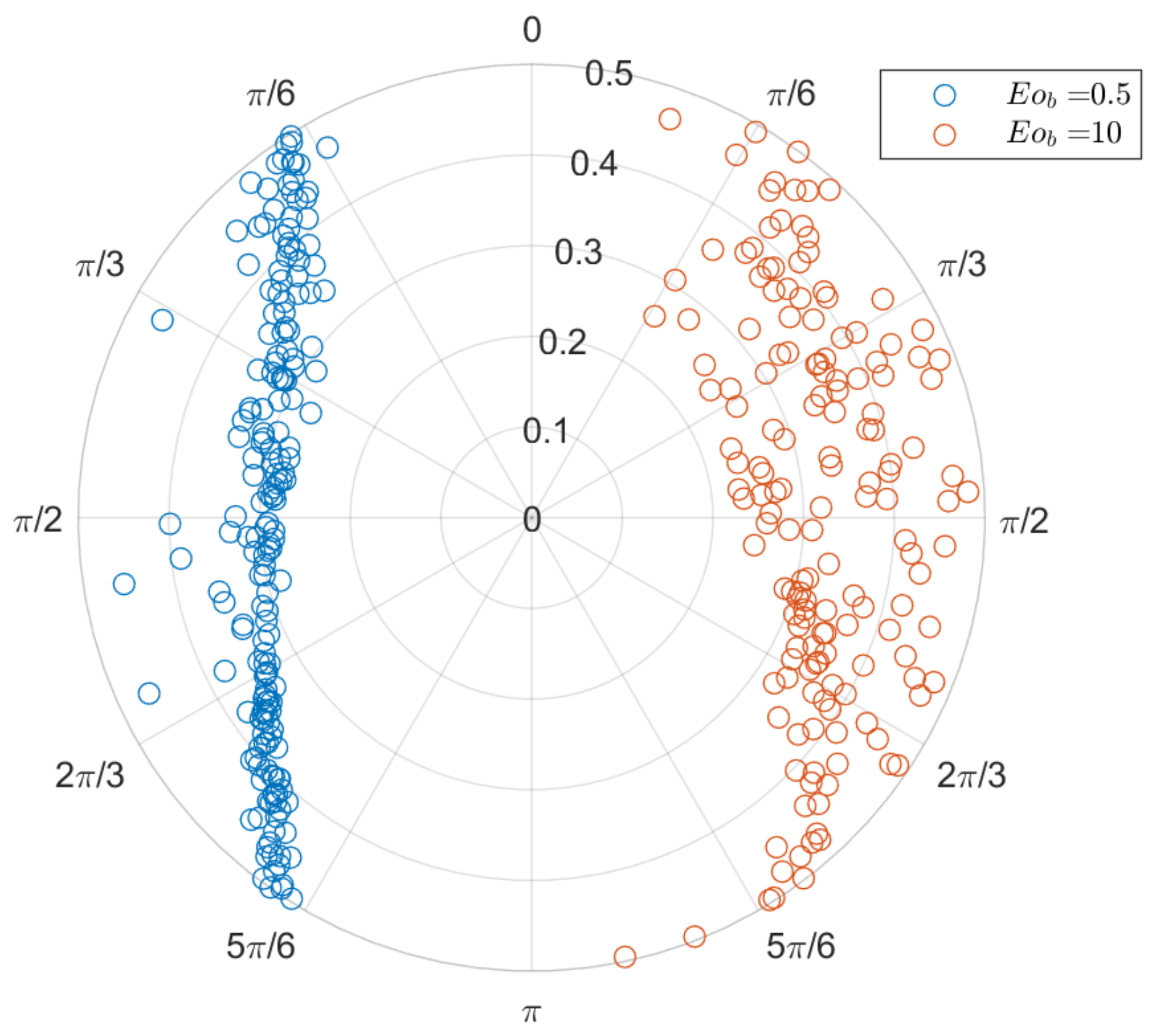
Figure 5 at 21 equispaced times, for 12 drops ( N d = 12 ). Data for E o b = 0.5 are shown on the left and for E o b = 10 on the right. In both cases, the drops move past the bubble, with essentially no drops directly ahead or behind the bubble. For the nearly spherical bubble, the drops are clustered in a relatively narrow column that almost touches the bubble since the sum of the bubble and drop radii is R b + R d = 0.3 , but for the more deformable bubble, the droplets are more spread out, and we see more drops closer to the centerline in front of the bubble. Since the high E o b bubble becomes relatively “flat” as it rises and can change its orientation, a few drops are found closer to the center than for the nearly spherical bubbles.
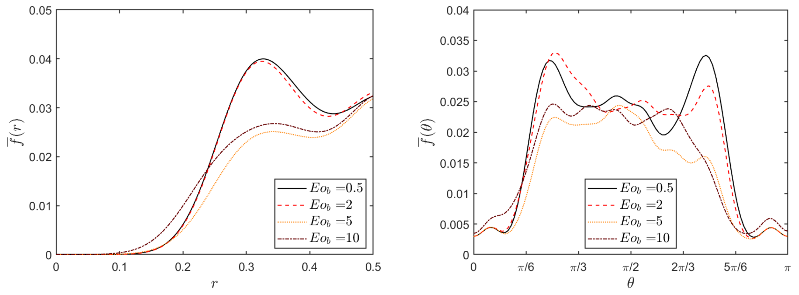
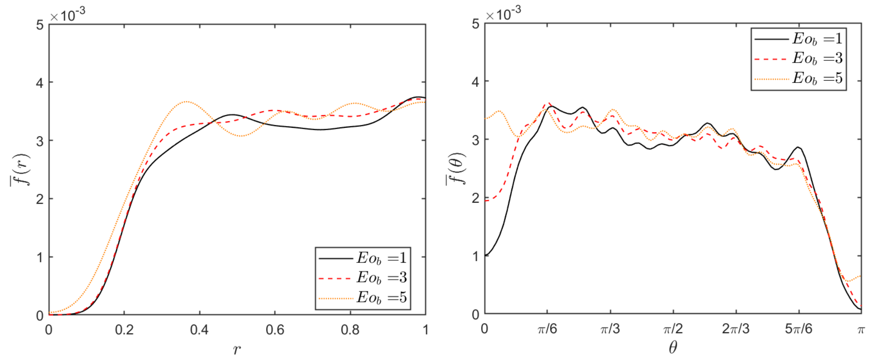
To examine the droplet distribution in more detail, we define a distribution function by
f ( r , θ , φ ) = 1 N d i = 1 , N d K δ ( x B x i )
where x B is the location of the bubble center, x i is where the center of drop i is, r is the distance of the drop center from the bubble center, and φ and θ are the azimuthal and polar angles, respectively. K is a smoothing kernel to produce a continuous curve, where the width of the kernel is selected by trial and error. When averaging over the azimuthal angle, we divide by 2 π r s i n θ to account for the dependency of the volume on the polar angle. The weighted average radial and angular distributions are shown in Figure 6. The left frame shows the radial distribution, averaged over the polar direction. The curves for the two lower E o b are similar, and the curves for the two higher E o b are similar. For the nearly spherical bubbles (lower E o b ), there is a distinct maximum at r = 0.3 , as also seen in Figure 5, but for the two higher E o b , the distribution is more uniform, and there are fewer drops close to the bubble. The angular distribution, averaged for r < 0.5 , is shown in the right frame, and it is clear that for the lower Eötvös numbers, the distribution is highest at around θ = π / 5 , then relatively uniform but with another peak at around θ = 4 π / 5 . At the poles, we see very low values, consistent with the left-hand side of Figure 5, which shows no drops there. For the higher E o b , the distribution is more uniform but tapers slightly off at the back.
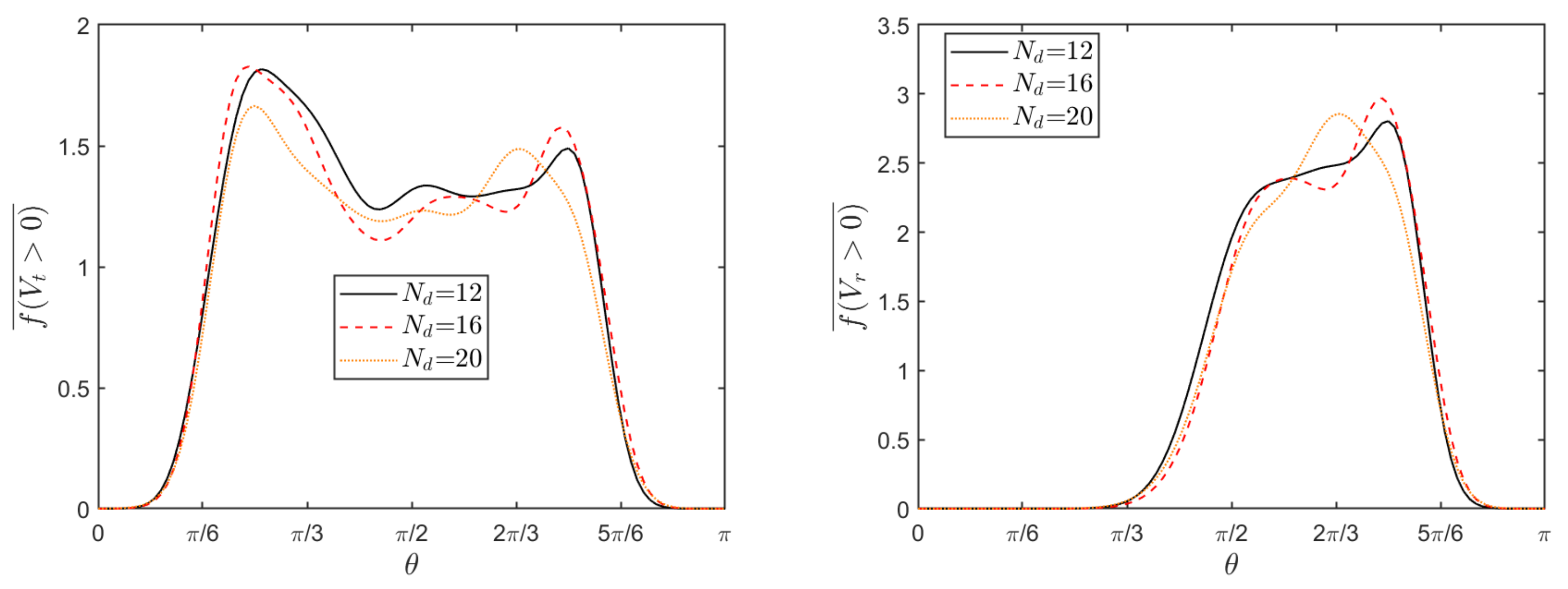
In Figure 7, we examine the effect of the number of drops on the relative velocity between the bubble and the drops by plotting the probability that the relative tangential velocity (left frame) and the relative radial velocity (right frame) are positive, following [6]. The tangential velocity is taken to be positive if the drop is moving toward the back of the bubble, and the radial velocity is positive if the drops move away from the bubble. In all cases, the plot on the left shows that the drops slide along the bubble surface from the front to the back, as expected, with the highest probability at around π / 5 . Similarly, the plot on the right shows that the drops are likely to be moving away from the bubble near its back but not the front, as expected. Overall the results show relatively weak dependency on the number of drops.

3.2. Several Bubbles and Drops

While examination of the interaction of several drops with one bubble in a “unit cell” allows us to study some aspects of the system with relatively little effort, in real systems, we expect to have several bubbles and many drops. Here, we present a few results for 8 freely moving bubbles and 48, 96, and 192 drops in fully periodic domains. The parameters are the same as in the previous section, and the bubble surface tension is varied to give different Eötvös and Morton numbers. Initially, the bubbles and the drops are located randomly in the domain. The simulations are run on 128 3 grids, up to time t = 100 at which time the bubbles have moved 10 times through the domain, on average. 
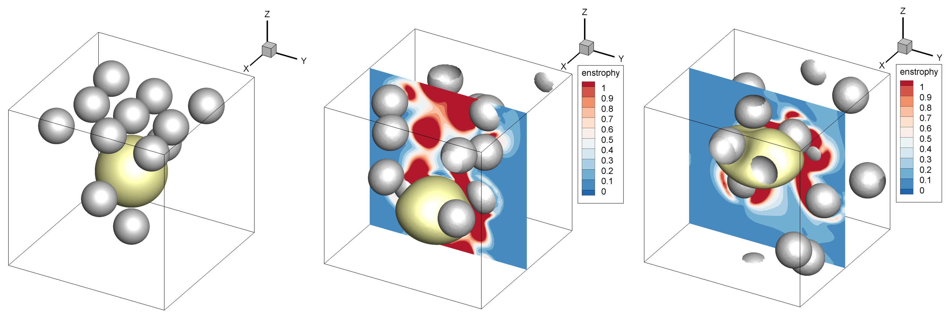
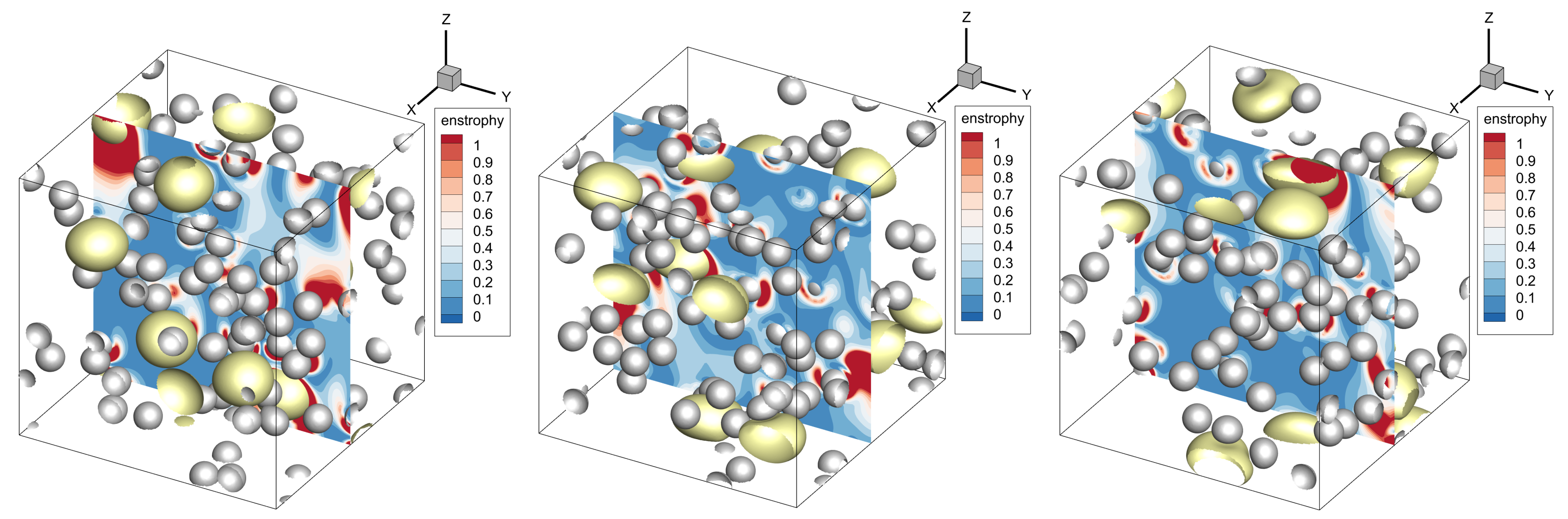
Figure 8 shows the solution at the last time simulated for E o b = 1.0 (left frame), E o b = 3.0 (middle frame), and E o b = 5.0 (right frame). In addition to showing the bubbles and the drops, we also show the enstrophy in a plane cutting through the middle of the domain. An examination of those plots, as well as others at different times, shows that overall, the flows are relatively similar. Both the bubbles and the drops are distributed throughout the domain, although small clusters of drops are often seen, such as here. Similarly, although sometimes the bubbles collide with each other, persistent clusters or “streams”, as sometimes found for deformable bubbles in fully three-dimensional flows, due to the differences in lift on spherical and deformable bubbles [30,31], are not seen. Although we do see regions of high vorticity, it is clear that it is not only concentrated in the wake of the bubbles, as we saw for the single bubble in a unit cell. We note that for the freely moving and interacting bubbles, we have not included results for E o b = 10 since the bubbles sometimes break, as they interact when the surface tension is low. While we believe that the breakup is physical, we have not implemented a topology change algorithm for the front in the current version of the code, since we do not want the number of bubbles and their sizes to change during each simulation.
The slip velocity between the bubbles and the continuous liquid, averaged over the eight bubbles, and the slip velocity between the drops and the continuous liquid, averaged over all the drops, are shown in the left frame of Figure 9 versus time for all 3 Eötvös numbers and 96 drops. In the right frame, the time average of the slip velocities is shown for E o b = 3 , versus the number of drops N d . The bubbles rise due to buoyancy, so their slip velocity is positive, while the drops are denser than the continuous liquid and fall down with a negative slip velocity. The left frame shows that the flow reaches a statistically stationary state very quickly, although the average bubble slip velocity fluctuates slightly. This is presumably due to the relatively small size of the system, both in terms of the number of bubbles and domain size. However, even in a larger system where the average over all the bubbles might be better converged, we still expect individual bubbles to move very unsteadily. The slip velocity of the drops fluctuates much less, in part because there are more of them, so the average is better converged. As the number of drops increases, the density of the liquid mixture (continuous liquid and drops) increases, but the resistance (or effective viscosity) of the droplet/continuous liquid mixture also increases, overcoming the increase in buoyancy and leading to a slight decrease of the average bubble slip velocity. Similarly, we see a very slight decrease in the average drop slip velocity. Plots of the average slip velocity versus E o b for a fixed N b (not included) show essentially no dependency on E o b . Although the flow reaches a stationary state quickly, the time average in the right frame has been computed between time t = 50 and t = 100 , using a time increment of Δ t = 0.0305 , except for the N d = 192 case, which was only run up to time 84.2 . The averages discussed below have all been computed in the same way.
The kinetic energy of the continuous liquid is plotted versus time in the left frame of Figure 10 for 96 drops and E o b = 1.0 , 3.0 , and 5.0 . For the nearly spherical bubbles ( E o b = 1 ), the fluctuations quickly reach a relatively constant level, but as the deformability of the bubbles increases, the kinetic energy initially becomes much larger, although for E o b = 3.0 , it then settles down to a similar value, as seen for the E o b = 1.0 case. For E o b = 5.0 , large-scale fluctuations seem to continue. We note that [30] found that the velocity fluctuations were much larger for deformable bubbles, as compared to nearly spherical ones, even when their rise velocity was similar and the deformable bubbles were distributed relatively uniformly in the computational domain (not in a “streaming” state). Figure 4 for a single bubble also shows similar differences in the average kinetic energy between nearly spherical bubbles (low E o b ) and more deformable ones (high E o b ). The time average of the kinetic energy of the continuous liquid is plotted in the right frame of Figure 10 versus N d for E o b = 3 . The dependency on the number of drops is relatively weak, although it increases slightly with N b . We note that the relatively large fluctuations and the short time over which the averaging is performed suggest a large uncertainty. Reducing the uncertainty would require a longer averaging time and/or a larger system, but we believe that the trend is correctly captured.
We also examined the distribution of drops around the bubbles. Figure 11 shows the locations of drops with respect to the center of a single bubble, at 11 evenly spaced times between t = 50 and t = 100 , for E o b = 1.0 on the left of the symmetry axis, and for E o b = 5.0 on the right. It is clear that the droplets are distributed relatively uniformly around the bubbles. There are drop-free regions in front and behind the bubbles, with the behind region slightly larger than the one in front, and a few more drops closer to the centerline for the more deformable bubbles. Thus, unlike for the single three-dimensional bubble in a “unit cell,” there is little dependency on the Eötvös number. This is shown by a more detailed analysis, such as by examining the average radial and polar distributions of the drops, f ( r ) and f ( θ ) averaged over the eight bubbles, shown in Figure 12 for different E o b and 96 drops. The radial distribution is shown in the frame on the left and the polar direction in the right frame, both found in the same way as in Figure 6 and smoothed in the same way using a kernel function. The radial distribution is nearly uniform and very similar for all three Eötvös numbers, but although the polar distribution is mostly similar, the probability of finding drops ahead of the bubble increases with its deformability ( E o b ).

4. Conclusions

We examined the dynamics of a three-phase system where buoyant bubbles and heavy drops move in a continuous liquid, focusing on the dynamics of relatively small systems where the drops do not collide and stick to, or engulf, the bubbles. In particular, we compared the slip velocity, the velocity fluctuations, and the distribution of drops around the bubbles for a simple “unit cell” where we used one bubble in a periodic domain, with a larger cell with eight freely moving bubbles. For one bubble in a cell the results show that bubble deformability has a strong impact on the distribution of drops around the bubble, but results for a larger number of freely moving and interacting bubbles show little effect of deformability and that the drops are relatively uniformly distributed with respect to the bubbles, for the parameters examined.
The main conclusions from the study is that for a system with freely evolving bubbles, the droplet distribution and the slip velocity of the drops and the bubbles is relatively insensitive to the bubble deformability and the volume fraction of drops, at least for the parameter examined here, and that while a unit cell captures reasonably well the effect of changing the bubble deformability and the number of drops, it does not predict accurately the average distribution of drops around each bubble. More studies, presumably using larger systems and longer simulation times, are needed to clarify the role of deformability on the velocity fluctuations. Moreover, in this study, we did not examine the effect of changing the gas volume fraction.

Author Contributions

Conceptualization, G.T.; methodology, G.T. and J.L.; software, J.L.; validation, J.L., L.Z. and D.V.; investigation, L.Z. and D.V.; writing—original draft preparation, G.T.; writing—review and editing, G.T. and L.Z.; project administration and funding acquisition, G.T. All authors have read and agreed to the published version of the manuscript.

Funding

This research was funded by NSF Grant CBET-2035231.

Conflicts of Interest

The authors declare no conflict of interest.

References

  1. Saththasivam, J.; Loganathan, K.; Sarp, S. An overview of oil-water separation using gas flotation systems. Chemosphere 2016, 144, 671–680. [Google Scholar] [CrossRef] [PubMed]
  2. Torza, S.; Mason, S. Three-phase interactions in shear and electrical fields. J. Colloid Interface Sci. 1970, 33, 67–83. [Google Scholar] [CrossRef]
  3. Moosai, R.; Dawe, R.A. Gas attachment of oil droplets for gas flotation for oily wastewater cleanup. Sep. Purif. Technol. 2003, 33, 303–314. [Google Scholar] [CrossRef]
  4. Yan, S.; Yang, X.; Bai, Z.; Xu, X.; Wang, H. Drop attachment behavior of oil droplet-gas bubble interactions during flotation. Chem. Eng. Sci. 2020, 223, 115740. [Google Scholar] [CrossRef]
  5. Yaqub, M.W.; Marappagounder, R.; Rusli, R.; Prasad, D.M.R.; Pendyala, R. Review on gas-liquid–liquid three-phase flow patterns, pressure drop, and liquid holdup in pipelines. Chem. Eng. Res. Des. 2020, 159, 505–528. [Google Scholar] [CrossRef]
  6. Bunner, B.; Tryggvason, G. Dynamics of Homogeneous Bubbly Flows: Part 1. Rise Velocity and Microstructure of the Bubbles. J. Fluid Mech. 2002, 466, 17–52. [Google Scholar] [CrossRef]
  7. Lu, J.; Tryggvason, G. Dynamics of nearly spherical bubbles in a turbulent channel upflow. J. Fluid Mech. 2013, 732, 166–189. [Google Scholar] [CrossRef]
  8. du Cluzeau, A.; Bois, G.; Toutant, A. Analysis and modelling of Reynolds stresses in turbulent bubbly up-flows from direct numerical simulations. J. Fluid Mech. 2019, 866, 132–168. [Google Scholar] [CrossRef] [Green Version]
  9. Rajesh, V.M.; Buwa, V.V. Volume-of-fluid simulations of gas-liquid–liquid flows in minichannels. Chem. Eng. J. 2018, 345, 688–705. [Google Scholar] [CrossRef]
  10. Li, H.Y.; Yap, Y.F.; Lou, J.; Shang, Z. Numerical modelling of three-fluid flow using the level-set method. Chem. Eng. Sci. 2015, 126, 224–236. [Google Scholar] [CrossRef]
  11. Tofighi, N.; Yildiz, M. Numerical simulation of single droplet dynamics in three-phase flows using ISPH. Comput. Math. Appl. 2013, 66, 525–536. [Google Scholar] [CrossRef]
  12. Dinariev, O.Y.; Evseev, N.V. Modelling of flotation processes by density functional hydrodynamics. Miner. Eng. 2018, 125, 239–251. [Google Scholar] [CrossRef]
  13. King, R. Modeling and Simulation of Mineral Processing Systems; Butterworth-Heinemann: Oxford, UK, 2012. [Google Scholar]
  14. Pita, F.; Castilho, A. Separation of plastics by froth flotation. The role of size, shape and density of the particles. Waste Manag. 2017, 60, 91–99. [Google Scholar] [CrossRef] [PubMed]
  15. van Sint Annaland, M.; Deen, N.; Kuipers, J. Numerical simulation of gas–liquid–solid flows using a combined front tracking and discrete particle method. Chem. Eng. Sci. 2005, 60, 6188–6198. [Google Scholar] [CrossRef]
  16. Liu, Q.; Luo, Z.H. CFD-VOF-DPM simulations of bubble rising and coalescence in low hold-up particle-liquid suspension systems. Powder Technol. 2018, 339, 459–469. [Google Scholar] [CrossRef]
  17. Lecrivain, G.; Yamamoto, R.; Hampel, U.; Taniguchi, T. Direct numerical simulation of a particle attachment to an immersed bubble. Phys. Fluids 2016, 28, 083301. [Google Scholar] [CrossRef] [Green Version]
  18. Bogner, S.; Harting, J.; Rüde, U. Direct simulation of liquid–gas–solid flow with a free surface lattice Boltzmann method. Int. J. Comput. Fluid Dyn. 2018, 31, 463–475. [Google Scholar] [CrossRef] [Green Version]
  19. Liu, T.; Schwarz, M. CFD-based modelling of bubble-particle collision efficiency with mobile bubble surface in a turbulent environment. Int. J. Miner. Process. 2009, 90, 45–55. [Google Scholar] [CrossRef] [Green Version]
  20. Liu, T.; Schwarz, M. CFD-based multiscale modelling of bubble-particle collision efficiency in a turbulent flotation cell. Chem. Eng. Sci. 2009, 64, 5287–5301. [Google Scholar] [CrossRef]
  21. Fayed, H.E.; Ragab, S.A. Direct Numerical Simulation of Particles-Bubbles Collisions Kernel in Homogeneous Isotropic Turbulence. J. Comput. Multiph. Flows 2013, 5, 167–188. [Google Scholar] [CrossRef]
  22. Maxwell, R.; Ata, S.; Wanless, E.; Moreno-Atanasio, R. Computer simulations of particle-bubble interactions and particle sliding using Discrete Element Method. J. Colloid Interface Sci. 2012, 381, 1–10. [Google Scholar] [CrossRef]
  23. Gao, Y.; Evans, G.M.; Wanless, E.J.; Moreno-Atanasio, R. DEM simulation of single bubble flotation: Implications for the hydrophobic force in particle-bubble interactions. Adv. Powder Technol. 2014, 25, 1177–1184. [Google Scholar] [CrossRef]
  24. Deen, N.G.; van Sint Annaland, M.; Kuipers, J. Direct numerical simulation of complex multi-fluid flows using a combined front tracking and immersed boundary method. Chem. Eng. Sci. 2009, 64, 2186–2201. [Google Scholar] [CrossRef]
  25. Baltussen, M.; Seelen, L.; Kuipers, J.; Deen, N. Direct Numerical Simulations of gas-liquid–solid three phase flows. Chem. Eng. Sci. 2013, 100, 293–299. [Google Scholar] [CrossRef]
  26. Sasic, S.; Sibaki, E.K.; Ström, H. Direct numerical simulation of a hydrodynamic interaction between settling particles and rising microbubbles. Eur. J. Mech. B-Fluids 2014, 43, 65–75. [Google Scholar] [CrossRef]
  27. Cazarez, O.; Montoya, D.; Vital, A.; Bannwart, A. Modeling of three-phase heavy oil-water-gas bubbly flow in upward vertical pipes. Int. J. Multiph. Flow 2010, 36, 439–448. [Google Scholar] [CrossRef]
  28. Wang, G.; Ge, L.; Mitra, S.; Evans, G.M.; Joshi, J.; Chen, S. A review of CFD modelling studies on the flotation process. Miner. Eng. 2018, 127, 153–177. [Google Scholar] [CrossRef]
  29. Tryggvason, G.; Scardovelli, R.; Zaleski, S. Direct Numerical Simulations of Gas-Liquid Multiphase Flows; Cambridge University Press: Cambridge, UK, 2011. [Google Scholar] [CrossRef]
  30. Bunner, B.; Tryggvason, G. Effect of Bubble Deformation on the Stability and Properties of Bubbly Flows. J. Fluid Mech. 2003, 495, 77–118. [Google Scholar] [CrossRef]
  31. Ervin, E.; Tryggvason, G. The Rise of Bubbles in a Vertical Shear Flow. ASME J. Fluid Eng. 1997, 119, 443–449. [Google Scholar] [CrossRef]
Figure 1. A bubble and 12 drops at time 0 (left) and 100 for E o b = 2 (middle) and E o b = 10 (right). The enstrophy is shown in a plane cutting through the center of the domain.
Fluids 06 00317 g001
Figure 2. The slip velocity versus time for E o b = 2 and N d = 12 .
Fluids 06 00317 g002
Figure 3. The time-averaged slip velocity versus bubble Eötvös number for N d = 12 (left) and versus number of drops ( N d ) for E o b = 2 (right).
Fluids 06 00317 g003
Figure 4. The kinetic energy in the liquid versus time for N d = 12 and several Eötvös numbers (left). The time-averaged kinetic energy versus N d for E o b = 2 (right).
Fluids 06 00317 g004
Figure 5. The relative location of the drops for 21 time samples for N d = 12 . E o b = 0.5 on the left and E o b = 10 on the right.
Fluids 06 00317 g005
Figure 6. The angular average distribution function versus distance from the bubble center (left) and radially average distribution function versus angle, measured from the top of the bubble (right).
Fluids 06 00317 g006
Figure 7. The probability that the relative tangential (left) and radial (right) velocities of the drops next to the bubble are positive, for E o b = 2.0 and different numbers of drops.
Fluids 06 00317 g007
Figure 8. 8 bubbles and 96 drops at time 100, for E o b = 1.0 (left), E o b = 3.0 (middle), and E o b = 5.0 (right). The enstrophy is shown in a plane cutting through the center of the domain.
Fluids 06 00317 g008
Figure 9. Slip velocity for the bubbles and the drops. Left: The slip velocity versus time for 96 drops and E o b = 1.0 , 3.0 and 5.0 . Right: The time-averaged slip velocity for E o b = 3.0 versus the number of drops N b .
Fluids 06 00317 g009
Figure 10. The kinetic energy of the liquid versus time for 96 drops and E o b = 1.0 , 3.0 and 5.0 (left) and the time-averaged kinetic energy versus the number of drops for E o b = 3.0 (right).
Fluids 06 00317 g010
Figure 11. The location of drops with respect to bubble centers. The drops at several times are shown in the left frame for E o b = 1.0 (blue circles on the left) and E o b = 5.0 (red circles on the right).
Fluids 06 00317 g011
Figure 12. The radial distribution (left) and the polar distribution (right), averaged around the bubble, for three Eötvös numbers.
Fluids 06 00317 g012
Table 1. The surface tension for the bubbles and the corresponding E o b and M b .
σ 0.040.010.006670.0040.002
E o b 0.52.03.05.010.0
M b 3.1 × 10 8 2.0 × 10 6 6.7 × 10 6 3.1 × 10 5 2.5 × 10 4
Publisher’s Note: MDPI stays neutral with regard to jurisdictional claims in published maps and institutional affiliations.

