Abstract
The Alber equation is a phase-averaged second-moment model used to study the statistics of a sea state, which has recently been attracting renewed attention. We extend it in two ways: firstly, we derive a generalized Alber system starting from a system of nonlinear Schrödinger equations, which contains the classical Alber equation as a special case but can also describe crossing seas, i.e., two wavesystems with different wavenumbers crossing. (These can be two completely independent wavenumbers, i.e., in general different directions and different moduli.) We also derive the associated two-dimensional scalar instability condition. This is the first time that a modulation instability condition applicable to crossing seas has been systematically derived for general spectra. Secondly, we use the classical Alber equation and its associated instability condition to quantify how close a given nonparametric spectrum is to being modulationally unstable. We apply this to a dataset of 100 nonparametric spectra provided by the Norwegian Meteorological Institute and find that the vast majority of realistic spectra turn out to be stable, but three extreme sea states are found to be unstable (out of 20 sea states chosen for their severity). Moreover, we introduce a novel “proximity to instability” (PTI) metric, inspired by the stability analysis. This is seen to correlate strongly with the steepness and Benjamin–Feir Index (BFI) for the sea states in our dataset (>85% Spearman rank correlation). Furthermore, upon comparing with phase-resolved broadband Monte Carlo simulations, the kurtosis and probability of rogue waves for each sea state are also seen to correlate well with the PTI (>85% Spearman rank correlation).
1. Introduction
Ocean waves are a very active field of mathematical modelling and analysis. The first principles of hydrodynamic models for gravity waves are by now well understood [1,2,3]. An array of approximate models are well established and widely used, including the nonlinear Schrödinger equation (NLS) and its variants [4,5], the Zakharov equation [6], the coupled-mode systems [7,8,9], the High Order Spectral Method (HOSM) [10,11,12] and others. (In shallow water, an even larger collection of models is being used, but here we focus on deep water.) One reason for the wide use of approximate models in oceanography is the need to study large wavefields, with hundreds or thousands of individual wavelengths. Thus, there is a trade-off between hydrodynamic fidelity and the ability to scale up models, as well as the accessibility of powerful qualitative insights.
In fact, actual ocean waves include multi-physics and nondifferentiable phenomena, such as wind forcing, wave breaking, etc. These are not accounted for in the classical “exact” hydrodynamic model anyway and understanding of them is still developing on different levels [13,14,15,16,17].
In this paper, we will use stochastic modelling of ocean waves and, furthermore, explore what phase-averaged stochastic models may reveal about rogue waves in particular. This will lead us to novel mathematical results; it is also worth mentioning that this kind of overall approach has been identified as a priority within the broader marine research and industry community [18].
The most well known stochastic models for ocean waves include the CSY equation [19,20,21], Hasselmann’s equation [22] and the Alber equation [23], which we will focus on here. For a recent review of various stochastic models, one can see [24]. Broadly speaking, they are moment equations, starting from phase-resolved equations for the sea surface (such as Zakharov’s equation or the NLS) as an approximation for deterministic wave dynamics. One then takes stochastic moments of the deterministic equations; due to the nonlinearity of these equations, an infinite hierarchy of moments is produced. A Gaussian second-order moment closure is then used to produce a closed equation for the second stochastic moment. The resulting equation is phase-averaged, meaning that it no longer resolves individual wave peaks and troughs, but instead the evolution and propagation of the statistics of the wavefield.
A key approximation step is the Gaussian moment closure. This is of course not exact, but in many cases the free surface is indeed close to being Gaussian [25,26], making the Gaussian closure plausible. It is important to keep in mind that fidelity to the deterministic, phase-resolved model is not the only consideration: for example, the exact infinite hierarchy of moments is not just more complicated as a mathematical model, it is impossible to initialize meaningfully. The vast majority of synoptic data collected from the ocean are, or can be converted to, some kind of second moment [26]. There are some data involving moderately higher moments, but very few data and little know-how exists for moments higher than fourth order.
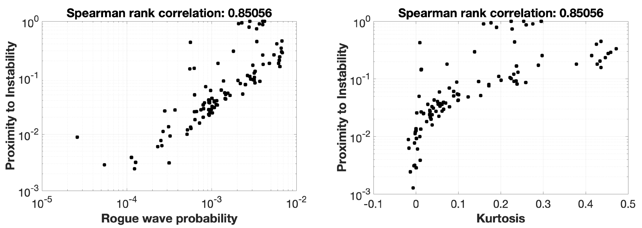
The question of using realistic data for initialisation is extremely important; all the more so in the study of extreme sea states and rogue waves. For example, every deterministic model can produce “rogue waves” on demand, by carefully preparing particular initial conditions; however, the real-life question is how often would these “initial conditions leading to rogue waves” realistically appear? A stochastic approach can directly answer this question e.g., by a phase-resolved Monte Carlo approach [27]; this has a number of advantages, but is clearly expensive to apply indiscriminately. Another possibility would be using phase-averaged stochastic models, such as the moment equations discussed above, to directly investigate whether a sea state could likely support the rapid concentrations of energy. In this way, sea states of interest could be selected and computational resources focused on them. In fact, it appears that the sea states highlighted as more unstable by the Alber equation turn out to exhibit a higher probability of extreme events in a phase-resolved Monte Carlo simulation (details in Section 3.2.3 and Figure 5).
2. Ocean Wave Modelling with the Alber Equation
The Alber equation, its derivation and interpretation have been widely studied and explained. We refer readers who are interested to [23,28,29,30] and the references therein for more details. Here, we will briefly present its derivation and main features in order to make the paper self-contained.
2.1. Derivation
The cubic focusing on the nonlinear Schrödinger equation (NLS)
is an approximate model for the envelope of a narrow-banded wavetrain with a carrier wavenumber along its direction of propagation (unidirectional propagation), cf. e.g., [31]. Thus, in deep water the sea surface elevation is related to the complex-valued envelope through
where and
This is an asymptotic model, where the order parameter is the steepness of the waves, and moreover assumes narrow-bandedness of the wavefield around the carrier wavenumber. The NLS and its variants are widely used as they are considered relevant to a wide array of realistic scenarios [27]. There are some key facts behind this: water waves cannot get too steep, since they break at a slope of about and typically they are less steep than that. Moreover, wavelengths for gravity waves vary over no more than two orders of magnitudes, ∼5–500 m. In fact, sea state spectra are known to often be more narrowly supported even within that range. In contrast, crossing seas (i.e., two wave systems coming from different directions) cannot be considered narrowband due to the different directions; thus, they provide a prime example of a realistic situation where the NLS (1) would not be a satisfactory model.
A different kind of limitation of the NLS is that it is a deterministic phase-resolved model—i.e., any prediction with it will not be better or more accurate than the initial condition used. However, realistic wave systems are not widely available as phase-resolved initial conditions, as opposed to power spectra. In this context, Alber [23] proposed generating a second-order moment equation from the NLS, considered with stochastic initial data. Denoting by
the autocorrelation of the envelope one obtains
By using the Gaussian closure
the autocorrelation can now be seen to satisfy
A key restriction the Alber equation inherits from its starting point, the NLS equation, is narrowbandedness. This is arguably not too restrictive for unidirectional sea states [27]; however, it completely fails for crossing seas, i.e., sea states where several different directions carry substantial wave energy. To address this limitation, we will derive a generalized Alber equation valid in a crossing seas scenario. This is made possible by starting from a system of NLS equations describing the crossing wavetrains which was derived in [32]. The resulting generalized Alber equation is reported in Section 3 and derived in detail in Section 4. Crossing seas are receiving increased attention as a possible incubator of rogue waves [33,34], so it is important to have a moment equation applicable to such scenarios.
2.2. The Stability-of-Homogeneity Question
It is empirically known that sea states are typically homogeneous and stationary, at least for appropriate length scales and timescales [25,26,35,36]. This feature is reflected in the Alber equation; for example, it can be seen is a solution of Equation (4) for any smooth function The next step is to investigate the stability of such homogeneous and stationary solutions: let us consider a weakly inhomogeneous initial sea state, i.e., assume that the autocorrelation is initially of the form
for some nice functions (e.g., Schwartz class test functions). By inserting Equation (5) into Equation (4), one can reformulate the problem in terms of the inhomogeneity
So, stability of homogeneous states is controlled by the boundedness (or lack thereof) of the inhomogeneity in Equation (6). Can grow in time to the extent that is no longer small? Or is there a guarantee that stays bounded? In the latter case of stability, the autocorrelation will simply stay close to for all times. In the unstable case, however, even if initially it is very close to homogeneous, the autocorrelation could develop significant inhomogeneities.
In [23], a sufficient condition for linear instability was derived in terms of the spectrum , namely the Fourier transform of the autocorrelation function
Indeed, it was shown that the homogeneous sea state with autocorrelation is unstable if, for some there exists so that
This was called an “eigenvalue relation” in [23]; we will call it an “instability condition”. In [30], it was further shown that if the instability condition does not hold, then linear stability follows. The instability condition (7) itself can be refined in two ways: One concerns a technical issue related to However, the more important one is that, in (7), we are asked to guarantee the existence or nonexistence of solutions for a nonlinear system of two equations (the real and imaginary parts of Equation (7)) in three real unknowns ( ). This is not straightforward in general, and historically it has been a challenge to use the Alber equation more widely [29]. In [30], this condition is reformulated so that a more constructive method to check it can be found: by dividing both sides of the fraction by X and setting
Equation (7) becomes
This becomes very simple if we recognize it as the Hilbert transform of the divided difference of a rescaled spectrum. So, denoting
and dropping the primes, the condition for instability finally becomes
The benefit is that now the argument principle (for a holomorphic function f defined on a closed domain it follows that if and only if the curve is circumscribed around z ) can be used to reformulate this to a constructive condition that we can directly check [30,37,38]. To this end, we will also need to introduce the signal transform
we are now ready to state the equivalent instability condition:
Definition 1
(Penrose–Alber condition). Consider a homogeneous sea state with an autocorrelation function and carrier wavenumber and denote Then, the sea state is Penrose–Alber unstable if
where
Any X for which is called an unstable wavenumber.
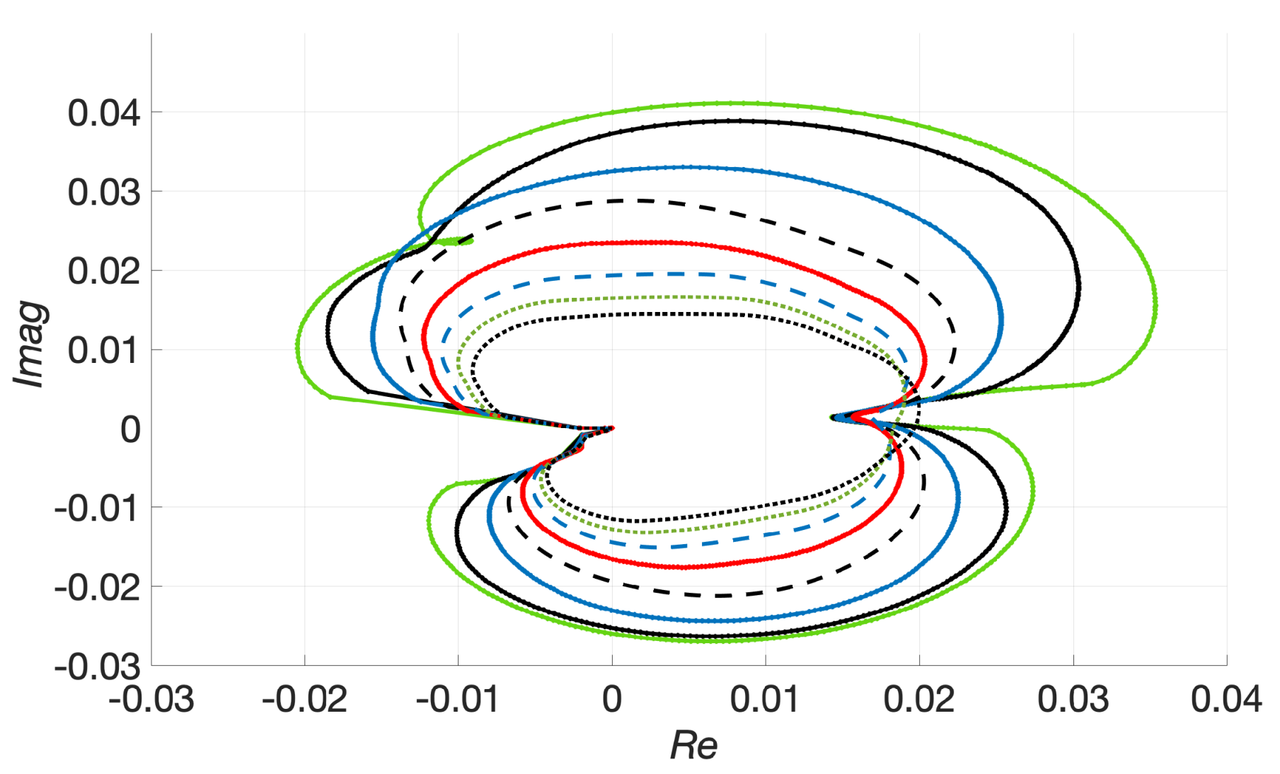
This notion of instability is equivalent to condition (9) [30]. The closed curves are visualized for a concrete example at the top of Figure 1.
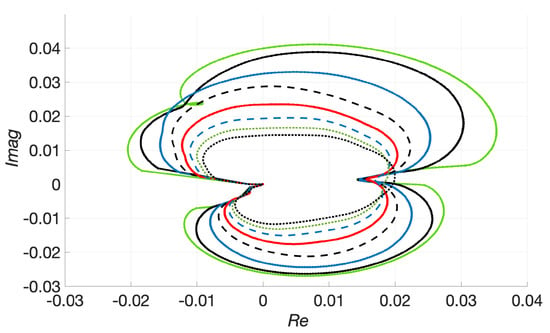
Figure 1.
Curves for a nonparametric spectrum on the complex plane. The smaller closed curves correspond to larger here, Taking does not change the outermost curve noticeably, as has effectively converged to The real number is not circumscribed by any of the curves, i.e., the spectrum does not exhibit modulation instability (cf. Definition 1). The spectrum used is a unimodal spectrum with a reference steepness of around taken out of the dataset of 100 nonparametric spectra.
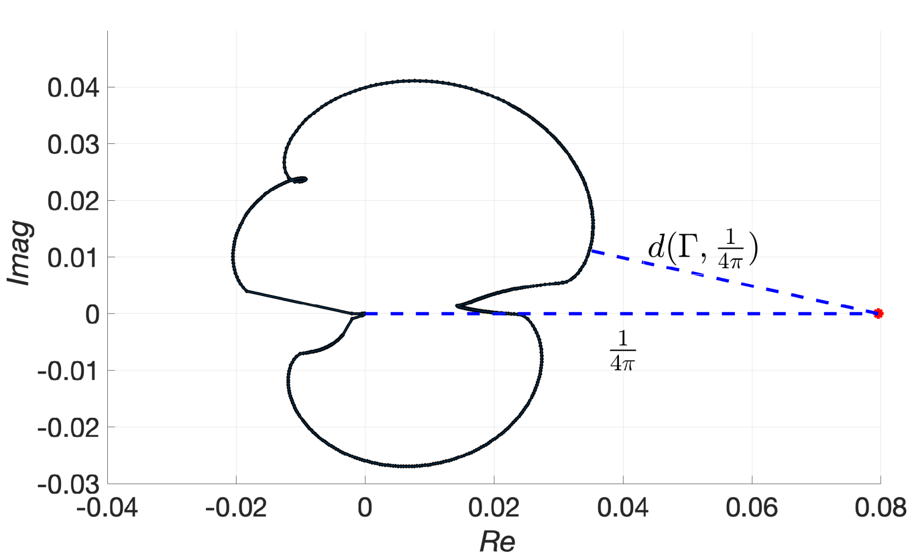
We call this the Penrose–Alber instability condition after Alber’s “eigenvalue relation” (7) [23] and Penrose’s introduction of the argument principle in an analogous problem in plasma [37]. The point with this is that this formulation of the condition boils down to drawing closed curves on the complex plane and looking at whether the point is inside or outside of them, cf. Figure 2. It was used in [30] to study parametric JONSWAP spectra; here, we will apply it to nonparametric spectra as well.
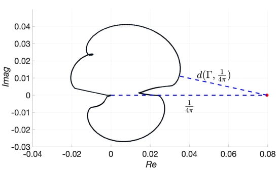
Figure 2.
We can quantify how close each spectrum is to being modulationally unstable by measuring the distance between and (plotted here as a red star). In practice, it suffices to carry this out for as much smaller values of X yield similar results, and large values of X lead to smaller and smaller curves, cf. Figure 1. So, now we can say that spectrum no. 11300 needs to be around in order to be modulationally unstable.
This stability-of-homogeneity question that was first studied in [23] is in fact a variant of a much better known stability question. The modulation instability (MI) is well understood and widely studied in a phase-resolved setting with a plane wave background [39]. It can easily be seen that a sequence of spectra approaching a plane wave would become unstable in the Penrose–Alber sense. In fact, the Penrose–Alber instability is just the modulation instability for more general backgrounds than plane waves. A modulationally unstable sea state supports the rapid concentrations of energy—a possible mechanism for the formation of rogue waves [38,40,41,42].
Unlike the classical MI, where every plane-wave solution is always unstable, a spectrum can be stable or unstable in the Penrose–Alber sense. In the case of stability, the homogeneity of the sea state is robust, and small perturbations will merely disperse. In these cases, despite having nonlinearity and infinite energy present, the dynamics are going to be dominated by the linear dispersion for all times. This is a familiar leading order approximation in ocean waves, but it does not necessarily have a name to itself in an oceanographic context. As the rigorous stability analysis of [30] highlighted, mathematically this stable regime looks exactly like what is called Landau damping for Vlasov equations (indeed this parallel was also drawn before [43]).
2.3. Implications
2.3.1. Quantifying Stability
As above, a key feature of the Alber equation is a classification of a given spectrum as either stable or unstable. A careful look at the asymptotics can offer more nuance. For example, consider two sea states: one with a barely stable spectrum and the other with a slightly perturbed version, e.g., so that it becomes barely unstable. These sea states will behave similarly on physically realistic timescales—as one would intuitively expect. In particular, there is not a violent bifurcation from Landau damping to modulation instability, but rather a gradual transition [30,38]. On the other hand, as we will see in some detail here, a spectrum exhibiting Landau damping can be “more stable” than another spectrum which also exhibits Landau damping. In short, the effective stability of a spectrum is better thought of as belonging to a continuous range of values rather than a binary “stable / unstable” classification. One of the results of this paper is a nondimensional index quantifying this “effective stability”, cf. Figure 2 and Figure 4.
This is important because, even in the presence of Landau damping (i.e., for “stable” spectra), only small enough inhomogeneities are guaranteed to disperse if the nonlinearity is taken into account. Large inhomogeneities are not well understood and could very well behave differently. This is a harder mathematical problem, because now, by definition, asymptotics are not sufficient. To better understand this question, there is a numerical requirement (efficient and reliable solvers for the Alber equation both in the stable and unstable regimes) as well as a dat a requirement (quantify how large inhomogeneities are in the ocean; this may be possible, e.g., with X-band radar imaging [44]). It is quite possible that, if a spectrum is close enough to MI, the likelihood of nonlinear events under realistic perturbations may substantially increase, even if technically the spectrum still exhibits Landau damping.
2.3.2. Nonparametric Spectra
The fundamental scaling of the problem shows that the vast majority of plausible sea states would be stable, in accordance with the well known fact that linearized dynamics very often do a good job in describing phase-averaged energy propagation. On the other hand, it seems that instability is within reach, i.e., the scaling of the problem does not make instability so far removed as to be considered impossible. This much was established in [28,29,30], working in the context of fitted parametric JONSWAP spectra. While fitted spectra are widely used, realistic spectra from the field come in many different shapes and forms. In this paper, we work with a set of nonparametric unidirectional spectra. We investigate whether they are stable or unstable in the Penrose–Alber sense, and proceed to examine how well the “proximity to instability” (defined more precisely in Equation (19)) correlates with the probability of rogue waves appearing in the given sea state.
The dataset, methodology and results of our investigation are described in detail in Section 3.2.
2.3.3. Emergence of Coherent Structures
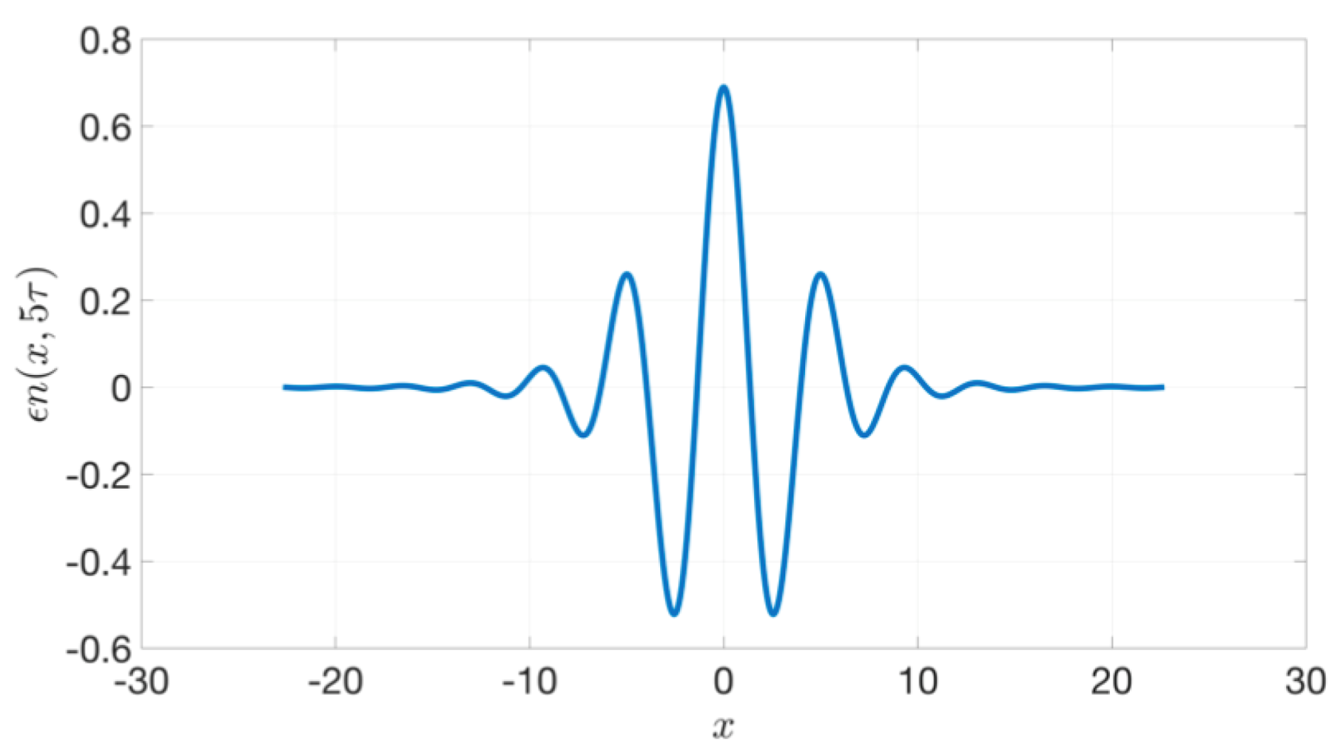
Another area with many open questions is what happens when instability arises. For modulationally unstable spectra with small inhomogeneity, formal asymptotics can be used to describe the early evolution of the instability. A particular coherent structure emerges, determined by the unstable wavenumbers for the particular spectrum and their rate of growth. In that sense, the coherent structure, at least in its early stages, is determined by the spectrum (and not by the inhomogeneity) and the Penrose–Alber instability analysis suffices to predict it [38]. Rather surprisingly, the same kind of universal coherent structure was reported in a fully numerical study by van den Eijden et al. [45], for the fully nonlinear stage of the instability, cf. Figure 3. This is a direction with many open questions, where more work is needed.

Figure 3.
Predicted profile of emergent localized extreme events for NLS, computed according to the methodology of [38]. A virtually identical universal profile of fully developed rogue waves is reported in Figure 2 of [45] for the largest extreme waves. This brings to mind the “three sisters” discussion [46,47,48,49,50,51], or the Greek .
3. Main Results
3.1. The Alber Equation for Crossing Seas
The original derivation of the Alber equation [23] allows for an oblique but small inhomogeneity on a unidirectional sea state. This does include some two-dimensional aspects; however, it does not allow for two large, different wavesystems, with different main directions of propagation, crossing. Such a situation is called “crossing seas” and is recently attracting a lot of interest. In particular, it is thought that modulation instability and rogue waves may be more prominent in crossing seas, but this is still very far from fully understood [32,33,34,41,52].
One way to study crossing seas is by deriving a coupled system of equations, each governing the evolution of one (quasi-uni-directional) wavefield. Let us denote the direction of propagation for the wavetrain A by and for the wavetrain B by The corresponding frequencies are
for ocean waves (i.e., in the limit of infinite depth). In [32], the following system of NLS equations for the envelopes of two wavetrains, in two spatial dimensions is derived:
All the coefficients are completely determined in terms of [32].
Theorem 1.
Consider the two crossing wavefileds of Equations (13) and (14), and assume moreover that their autocorrelations at can be written as
where are defined in terms of the data of the problem in Equation (47). In that case, inhomogeneities are expected to grow in time.
On the other hand, if
and
hold, then formally the problem exhibits linear Landau damping, i.e., inhomogeneities are expected to disperse and thus deviation from homogeneity is expected to not grow noticeably.
The proof is found in Section 4.
Remark 1.
Roughly speaking, and are transfer functions generated by the homogeneous backgrounds and express the free space (i.e., ) evolution of the initial inhomogeneities.
Furthermore, condition (17) is a Penrose–Alber condition for a system, and it is consistent with the condition for the scalar case. To see this, assume that then, according to the definition of (cf. Equation (47)) as well, the condition becomes
which is exactly of the same type as requiring
in the scalar case.
Just like in the scalar case, Condition (17) can also be resolved with the argument principle since, for each it asks whether a holomorphic function attains the value 0 on the right half-plane, . Condition (18) apparently boils down to general regularity conditions for the spectra Working these ideas out in full detail will require the extension of some technical results to a nonstandard “two-dimensional Hilbert transform” which arises here.
3.2. Stability of Unidirectional Nonparametric Spectra and Proximity to Instability (PTI)
3.2.1. The Data
For the present analysis we have used 100 realistic nonparametric spectra taken from the Norwegian Meteorological Institute’s operational spectral wave model [53], which is a third-generation wave model based on WAM. The model provides wave spectra every hour for many locations in the North Atlantic. For this study, 100 spectra from one specific location south-west of the Norwegian coast (5636 N, 312 E) were used. The selected spectra consisted of 80 spectra randomly selected from the full database (26,255 spectra covering the period from October 2016 to September 2019), as well as the 10 spectra having the largest mean wave steepness and the 10 spectra with the largest BFI values. Recall that the Benjamin–Feir Index (BFI) was defined from the frequency spectrum as
where is a measure for the frequency bandwidth here defined in terms of Godas’ peakedness factor , as suggested, e.g., in [54]:
and where is the total energy of the spectrum.
Note that for the following analysis the original frequency spectra were converted into wavenumber spectra using the linear dispersion relation .
3.2.2. The Algorithm for Checking the Instability Condition
Here, we will implement the stability criterion of Definition 1 to a number of nonparametric ocean spectra. First of all we will rescale them Actually, the selection of is a nontrivial issue. For example, one could plausibly use the mode, the mean or the median wavenumber. For narrow, unimodal spectra the choice would make very little difference, but for more irregular shapes, including, e.g., bimodal spectra, the resulting differences might be noticeable. In this case, we use the provided in the dataset by the Norwegian Meteorological Institute, which has been used for the computation of the BFI, steepness contained in the dataset, etc.
Once is determined and the rescaling is complete, we will need to interpolate the discrete data to a finer grid. (The original discrete spectra come sampled in 36 nonuniformly spaced wavenumbers.) This will be crucial in using effective quadrature methods. Splines are well suited to this task; the additional requirement is to minimize overshooting at maxima, as this could make a big difference with regard to our investigation. To this end, we use pchip, a piecewise polynomial interpolation routine in MATLAB that minimizes overshoot.
The nontrivial part of the computation is the Hilbert transform, which is a singular integral. To this end we will use the Sokhotski–Plemelj formula,
and truncate the limit by taking an appropriate After extensive testing it was found that the result did not change noticeably once . In this way, we avoided the singular integral. A detailed pseudocode for how the curve is generated is presented in Algorithm 1.
It is a moderately heavy computation if a good approximation for all of is required, as a few million points are typically required in order to achieve stringent error tolerances (∼10 relative error tolerance or ∼10 absolute error tolerance). However, one can check stability more quickly by checking only the points where these are the points where the curve crosses the real axis. If it never crosses the real axis to the right of then topologically cannot possibly be in the interior of the curve.
Some more details involve the selection of it was found that will produce the curves that have the most chance of coming closer to as when X increases the curves shrink to zero, see Figure 1. Numerical testing shows that gives a good picture of what happens as So, if for is not winding around nor coming very close to it, we can accept the spectrum as stable.
3.2.3. Summary of the Results
Most of the nonparametric spectra examined were found to be stable, i.e., exhibit Landau damping. However, three spectra were found to be modulationally unstable, and a handful more were extremely close to being unstable.
We also define as proximity to instability (PTI) the quantity
this is 1 for any modulationally unstable spectrum, and 0 for the zero spectrum. It provides a nondimensional way to quantify how close a spectrum comes to being modulationally unstable in the sense of Definition 1. We will compare this with quantities of interest for the same spectrum (cf. Figure 4), along with a Monte Carlo estimation of the likelihood of rogue waves and nonlinear events (cf. Figure 5).
| Algortithm 1. Pseudo-code for the computation of |
| Input (Sampled values of wavenumber-resolved spectrum, ) |
| Rescale ( is simply taken to be the peak wavenumber.) |
| Interpolate |
| Set compl_tol, rel_tol, abs_tol |
| For to step |
| While rel_err > rel_tol AND abs_err > abs_tol |
| Integrate one, generating two approximations, I_fine and I_coarse. (Fine grid has the number of points compared to coarse grid.) |
| Set |
| End While |
| Set |
| End For |
| Plot the line and the point |
| Check whether is inside (This can be achieved with the MATLABinpolygon function.) |
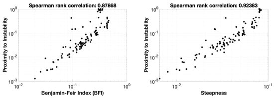
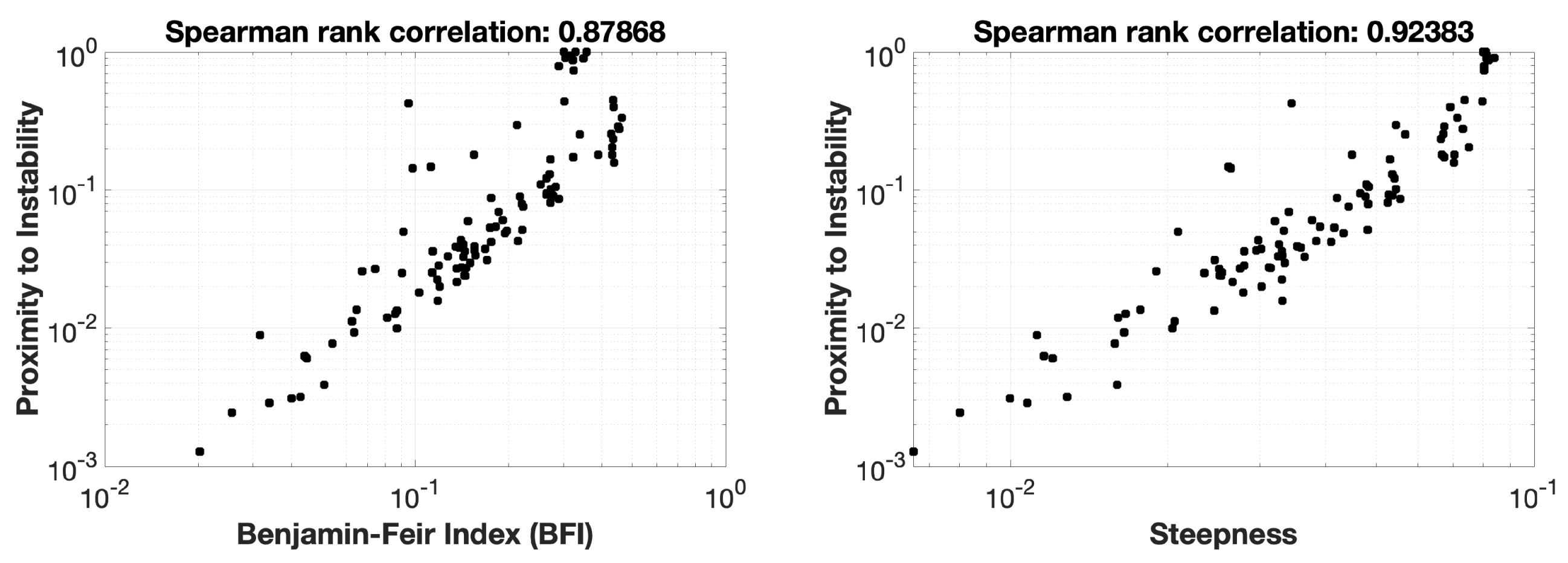
Figure 4.
The new metric of PTI offers a quantitative and nondimensional way to assess how far a spectrum is from being modulationally unstable. The Benjamin-Feir Index (BFI), essentially a rescaled version of steepness, was introduced with a similar task in mind; so, it is only natural to ask how well the two are correlated. In the left graph above, we see a log-log scatterplot of the BFI vs. PTI. In the right graph we see a similar scatterplot of a representative wave steepness, vs. PTI.

Figure 5.
Comparison of PTI to Monte Carlo results, please see Section 3.2.3 for more details on how these are defined and computed. Left: Rogue wave probability (understood as ) vs. PTI. Right: Kurtosis vs. PTI. See Section 3.2.3 for more details and context.
Indeed, for each of the 100 spectra selected for this study, we have run numerical simulations with the Higher Order Spectral Method (HOSM) [10,11] in a Monte Carlo approach where each spectrum was simulated 100 times with different initial random phases and random amplitudes run. That is, for a given spectrum , the initial surface elevation is in the form
where is the grid spacing between the discrete wavenumbers and where represents independent complex standard normal variables. That is, the real and imaginary parts of are independent normally distributed random variables with zero mean and variance , meaning that are Rayleigh distributed with parameter so that and and the phases are uniformly distributed on .
HOSM applies a regular discretisation of the wavenumbers so that , leading to a periodic domain of length in space. In the present simulations, we used , representing wavenumbers up to . This means that , corresponding to and , where is the reference wavelength.
Each simulation was run for 30 min, from which time series of surface elevation were extracted from four locations distributed over the simulation domain. Thus, 200 h of surface elevation time series were obtained for each sea state. Since here we are interested in relations between the instability (or proximity of such) obtained from the stochastic approach (i.e., Alber equation) and the occurrence of rogue and extreme events in random realisations of the sea states (i.e., phase-resolved Monte Carlo simulations), we will consider the following parameters related to the occurrence of extreme wave events: the sea surface kurtosis and the probability of extreme wave crests.
The sea surface kurtosis is a measure of how much the tail of the distribution deviates from Gaussian statistics. For a Gaussian distribution, the kurtosis is equal to zero, while a positive value for kurtosis indicates more large events than in a Gaussian population. Hence, the kurtosis is often used as an indicator for the probability of extreme and rogue waves.
Secondly, we consider the probability that a wave crest, defined as the maximum between each zero-crossing of the surface elevation, exceeds the significant wave height ; Recall that wave height is defined as the difference between a local maximum and a subsequent local minimum, i.e., in a sine wave it would be equal to two wave crests. Moreover, the significant wave height is defined as the mean value of the highest of wave heights. This is a common definition of a rogue wave, which under linear and Gaussian assumptions (Rayleigh distributed crests) has the probability . The probability of crest exceedance is estimated as the relative frequency of individual crests in the HOSM simulations that exceed the threshold . For brevity, we will refer to this probability simply as “rogue wave probability”.
4. Proof of Theorem 1
First of all, it should be noted that, by virtue of a simple gauge transform,
we can eliminate the terms with the first derivatives. Indeed, by inputting (21) into Equation (13), we see that eliminating the linear terms containing A and leads to
The first two lines represent a system, and for the third, nonlinear equation we only need to substitute the obtained values from above. The same steps lead to a symmetric expression for
Thus, without loss of generality, we will work with the simplified system
Special symmetric cases of this system which simplify the coefficients have been studied in [41,52], but we can in fact derive an Alber system for the general case.
To proceed, we will use some shorthand notations, namely
At this point, let us introduce the autocorrelation functions for
It can be seen that the relationship with the autocorrelations of the original variables is
and similarly for
By a straightforward computation, we see that
The last two lines consist of fourth order stochastic moments, and it is these terms that will have to be approximated by some closure scheme. For the fourth order moments involving A only, we will use the same idea as in the standard Alber equation; namely, we will use the fact that for Gaussian processes the relationship
holds (cf. Theorem A1). This now provides the Gaussian closure for all terms of the same form, since
follows the same argument. The new kinds of terms that come into play for the first time are the joint moments. In physical terms, A and B represent two different wavetrains meeting in the ocean, each having been generated and propagated independently from each other. It is thus a reasonable assumption that they are stochastically independent. In that case, the joint moments simplify to
So, using these closures, we finally end up with the following equation (whenever the independent variables are not shown explicitly, it is understood that ):
Now, we invoke the assumption of Equation (15), i.e.,
where now are the inhomogeneous components of the autocorrelation (recall that the conversion between second moments of and follows Equation (26)). It should be noted, under the condition (32), the system (30) and (31) is equivalent to (like earlier, and similarly for )
and is a solution. Following the terminology of Wigner equations, the terms
will be called position densities; they are real values, and they control the RMS amplitude of the inhomogeneities, for each wavetrain, on the coordinates
The question that we will focus on is whether is a linearly stable solution. To this end, we will consider nonzero initial data We will also need to introduce the change of variables
which leads to
and similarly for So, finally we arrive at the following system in the variables ():
Finally, by linearising (setting ) and taking the Fourier transform of both variables,
we obtain
where of course and similarly for Moreover, it can be seen that
hence, the notation
is natural. Additionally, in the interest of brevity, let us introduce the bilinear forms
Now, taking the Laplace transform in time
we obtain the system
By dividing with the free-space part we obtain
The two key observations here are the following:
- The rhs of both equations correspond to the linear free-space solutions (and thus can be treated as known and well behaved functions);
- We can now integrate both equations in the variables and obtain a closed system for the position densities achieving this is in fact the motivation for all the transforms and changes of variables.
We can summarize the result by denoting
so that system (46) becomes
leading to
as long as the determinant (itself a function of ) is nonzero,
If both Conditions (17) and (18) hold, then
inherit an -type decay in time, and one expects that Landau damping estimates similar to what was carried out in the scalar case in [30] are possible. Even without the rigorous estimates, one readily sees that there is no exponential growth possible, i.e., no modulation instability.
5. Conclusions
Using the same approach as in the classical Alber equation, we derived a system applicable to crossing seas, i.e., two quasi-unidirectional wave systems meeting in the ocean. This is a genuinely two-dimensional situation, and we produce for the first time the stability condition that controls whether Landau damping or modulation instability is present. This enables, for the first time, a systematic detection of modulation instability in crossing seas, including realistic data. Such a study is now made possible but involves several tedious steps that are beyond the scope of the current paper.
In this paper, we also study a collection of nonparametric unidirectional spectra; this can be thought of as a first step towards the study of the two-dimensional situation. The first subtlety that becomes apparent is that the choice of the carrier wavenumber, is an important aspect that can affect the results in a non-negligible way. (For example, the mean, mode or median wavenumbers are all plausible choices, and we did see spectra where these were significantly different, and would even lead to different stability/instability classifications for a handful of spectra.) Here we used the provided by the Norwegian Meteorological Institute and found that the vast majority of spectra in our collection are stable; however, among the most extreme sea states, it is possible to find spectra that would be classified as (barely) unstable. This is in agreement with the main findings of [30,38] and indicates that the Penrose–Alber instability really is a limiting factor of how narrow a spectrum can be in the ocean. The fact that there exist spectra all the way up to instability places additional emphasis on the question of how would unstable (or even borderline stable) spectra behave in the field, something that is really not well understood at all.
Moreover, we find that the novel Proximity to Instability (PTI) metric, defined in Equation (19), correlates well (>85% Spearman rank correlation) with the Benjamin–Feir Index (BFI) and the steepness of a sea state, as well as with Monte Carlo estimates for the kurtosis and the probability of rogue waves. This validates the PTI as a meaningful metric for the study of sea states in the unidirectional setting, where things are relatively well understood.
Given that now we have a version of the Alber equation (and the corresponding stability condition) applicable to crossing seas, the natural next step is to investigate crossing sea situations and see how well a generalized version of the PTI metric would correlate, e.g., with Monte Carlo estimates of the probability of rogue waves appearing there, as well as directional generalisations of the BFI [55,56]. Another option for this kind of analysis would be by working with the stability condition for the broadband Crawford–Saffman–Yuen equation (CSY) [19,21].
Author Contributions
Conceptualization, A.G.A. and O.G.; methodology, A.G.A. and O.G.; software, A.G.A. and O.G.; formal analysis & derivation, A.G.A.; investigation, A.G.A. and O.G.; resources, O.G.; writing—original draft preparation, review and editing, A.G.A. and O.G. All authors have read and agreed to the published version of the manuscript.
Funding
This research received no external funding.
Acknowledgments
We thank the Norwegian Meteorological Institute for providing the wave model spectra used in this study.
Conflicts of Interest
The authors declare no conflict of interest.
Appendix A
Theorem A1
(A complex Isselris theorem). Following [57]; see also [58]. Let be a Gaussian, zero mean, stationary process with the additional property that
Then
References
- Alazard, T.; Burq, N.; Zuily, C. On the Cauchy problem for gravity water waves. Invent. Math. 2014, 198, 71–163. [Google Scholar] [CrossRef]
- Lannes, D. Well-posedness of the water-waves equations. J. Am. Math. Soc. 2005, 18, 605–654. [Google Scholar] [CrossRef]
- Luke, J.C. A variational principle for a fluid with a free surface. J. Fluid Mech. 1967, 27, 395–397. [Google Scholar] [CrossRef]
- Benney, D.J.; Newell, A.C. The propagation of nonlinear wave envelopes. Stud. Appl. Math. 1967, 46, 133–139. [Google Scholar] [CrossRef]
- Trulsen, K.; Dysthe, K.B. A modified nonlinear Schrödinger equation for broader bandwidth gravity waves on deep water. Wave Motion 1996, 24, 281–289. [Google Scholar] [CrossRef]
- Zakharov, V.E. Stability of periodic waves of finite amplitude on the surface of a deep fluid. J. Appl. Mech. Tech. Phys. 1968, 9, 190–194. [Google Scholar] [CrossRef]
- Athanassoulis, G.A.; Belibassakis, K.A. A consistent coupled-mode theory for the propagation of small-amplitude water waves over variable bathymetry regions. J. Fluid Mech. 1999, 389, 275–301. [Google Scholar] [CrossRef] [Green Version]
- Athanassoulis, G.A.; Papoutsellis, C.E. Exact semi-separation of variables in waveguides with non-planar boundaries. Proc. R. Soc. Math. Phys. Eng. Sci. 2017, 473, 20170017. [Google Scholar] [CrossRef] [Green Version]
- Papoutsellis, C.E.; Charalampopoulos, A.G.; Athanassoulis, G.A. Implementation of a fully nonlinear Hamiltonian Coupled-Mode Theory, and application to solitary wave problems over bathymetry. Eur. J. Mech. B/Fluids 2018, 72, 199–224. [Google Scholar] [CrossRef] [Green Version]
- Dommermuth, D.G.; Yue, D.K.P. A high-order spectral method for the study of nonlinear gravity waves. J. Fluid Mech. 1987, 184, 267–288. [Google Scholar] [CrossRef]
- West, B.J.; Brueckner, K.A.; Janda, R.S.; Milder, D.M.; Milton, R.L. A new numerical method for surface hydrodynamics. J. Geophys. Res. Ocean. 1987, 92, 11803–11824. [Google Scholar] [CrossRef]
- Gouin, M.; Ducrozet, G.; Ferrant, P. Development and validation of a non-linear spectral model for water waves over variable depth. Eur. J. -Mech. 2016, 57, 115–128. [Google Scholar] [CrossRef] [Green Version]
- Brunetti, M.; Marchiando, N.; Berti, N.; Kasparian, J. Nonlinear fast growth of water waves under wind forcing. Phys. Lett. Sect. Gen. At. Solid State Phys. 2014, 378, 1025–1030. [Google Scholar] [CrossRef] [Green Version]
- Brunetti, M.; Kasparian, J. Modulational instability in wind-forced waves. Phys. Lett. Sect. Gen. At. Solid State Phys. 2014, 378, 3626–3630. [Google Scholar] [CrossRef] [Green Version]
- Armaroli, A.; Eeltink, D.; Brunetti, M. Nonlinear stage of Benjamin-Feir instability in forced/damped deep-water waves. Phys. Fluids 2018, 30, 017102. [Google Scholar] [CrossRef] [Green Version]
- Bühler, O.; Shatah, J.; Walsh, S.; Zeng, C. On the Wind Generation of Water Waves. Arch. Ration. Mech. Anal. 2016, 222, 827–878. [Google Scholar] [CrossRef] [Green Version]
- Janssen, P.A.E.M. The Interaction of Ocean Waves and Wind; Cambridge University Press: Cambridge, UK, 2004. [Google Scholar]
- Greenslade, D.; Hemer, M.; Babanin, A.; Lowe, R.; Turner, I.; Power, H.; Young, I.; Ierodiaconou, D.; Hibbert, G.; Williams, G.; et al. 15 Priorities for Wind-Waves Research: An Australian Perspective. Bull. Am. Meteorol. Soc. 2020, 101, E446–E461. [Google Scholar] [CrossRef] [Green Version]
- Crawford, D.R.; Saffman, P.G.; Yuen, H.C. Evolution of a random inhomogeneous field of nonlinear deep-water gravity waves. Wave Motion 1980, 2, 1–16. [Google Scholar] [CrossRef]
- Andrade, D.; Stiassnie, M. Bound-waves due to sea and swell trigger the generation of freak-waves. J. Ocean. Eng. Mar. Energy 2020, 6, 399–414. [Google Scholar] [CrossRef]
- Andrade, D.; Stiassnie, M. New solutions of the C.S.Y. equation reveal increases in freak wave occurrence. Wave Motion 2020, 97, 102581. [Google Scholar] [CrossRef]
- Hasselmann, K. On the non-linear energy transfer in a gravity-wave spectrum Part 1. General theory. J. Fluid Mech. 1962, 12, 481–500. [Google Scholar] [CrossRef]
- Alber, I.E. The Effects of Randomness on the Stability of Two-Dimensional Surface Wavetrains. Proc. R. Soc. Math. Phys. Eng. Sci. 1978, 363, 525–546. [Google Scholar] [CrossRef]
- Stuhlmeier, R.; Vrecica, T.; Toledo, Y. Nonlinear Wave Interaction in Coastal and Open Seas: Deterministic and Stochastic Theory. In Nonlinear Water Waves; Springer: Berlin/Heidelberg, Germany, 2019; pp. 151–181. [Google Scholar] [CrossRef] [Green Version]
- Komen, G.J.; Cavaleri, L.; Donelan, M.; Hasselmann, K.; Hasselmann, S.; Janssen, P.A.E.M. Dynamics and Modelling of Ocean Waves; Cambridge University Press: Cambridge, UK, 1994. [Google Scholar]
- Ochi, M.K. Ocean Waves: The Stochastic Approach; Cambridge University Press: Cambridge, UK, 1998; p. 332. [Google Scholar]
- Toffoli, A.; Gramstad, O.; Trulsen, K.; Monbaliu, J.; Bitner-Gregersen, E.; Onorato, M. Evolution of weakly nonlinear random directional waves: Laboratory experiments and numerical simulations. J. Fluid Mech. 2010, 664, 313–336. [Google Scholar] [CrossRef]
- Ribal, A.; Babanin, A.V.; Young, I.; Toffoli, A.; Stiassnie, M. Recurrent solutions of the Alber equation initialized by Joint North Sea Wave Project spectra. J. Fluid Mech. 2013, 719, 314–344. [Google Scholar] [CrossRef]
- Gramstad, O. Modulational Instability in JONSWAP Sea States Using the Alber Equation. In Proceedings of the ASME 2017 36th International Conference on Ocean, Offshore and Arctic Engineering, Trondheim, Norway, 25–30 June 2017. [Google Scholar]
- Athanassoulis, A.G.; Athanassoulis, G.A.; Ptashnyk, M.; Sapsis, T. Strong solutions for the Alber equation and stability of unidirectional wave spectra. Kinet. Relat. Model. 2020, 13, 703–737. [Google Scholar] [CrossRef]
- Mei, C.C.; Stiassnie, M.; Yue, D.K.P. Theory and Applications of Ocean Surface Waves; Advanced Series on Ocean Engineering; World Scientific: Singapore, 2005; Volume 23. [Google Scholar] [CrossRef]
- Hammack, J.L.; Henderson, D.M.; Segur, H. Progressive waves with persistent two-dimensional surface patterns in deep water. J. Fluid Mech. 2005, 532, 1–52. [Google Scholar] [CrossRef] [Green Version]
- Onorato, M.; Proment, D.; Toffoli, A. Freak waves in crossing seas. Eur. Phys. J. Spec. Top. 2010, 185, 45–55. [Google Scholar] [CrossRef]
- Gramstad, O.; Bitner-Gregersen, E.; Trulsen, K.; Nieto Borge, J.C. Modulational Instability and Rogue Waves in Crossing Sea States. J. Phys. Oceanogr. 2018, 48, 1317–1331. [Google Scholar] [CrossRef]
- Labeyrie, J. Stationary and transient states of random seas. Mar. Struct. 1990, 3, 43–58. [Google Scholar] [CrossRef]
- Tournadre, J. Time and space scales of significant wave heights. J. Geophys. Res. 1993, 98, 4727–4738. [Google Scholar] [CrossRef]
- Penrose, O. Electrostatic Instabilities of a Uniform Non-Maxwellian Plasma. Phys. Fluids 1960, 3, 258–265. [Google Scholar] [CrossRef]
- Athanassoulis, A.G.; Athanassoulis, G.A.; Sapsis, T. Localized instabilities of the Wigner equation as a model for the emergence of Rogue Waves. J. Ocean. Eng. Mar. Energy 2017, 3, 353–372. [Google Scholar] [CrossRef] [Green Version]
- Zakharov, V.E.; Ostrovsky, L.A. Modulation instability: The beginning. Phys. D Nonlinear Phenom. 2009, 238, 540–548. [Google Scholar] [CrossRef]
- Onorato, M.; Waseda, T.; Toffoli, A.; Cavaleri, L.; Gramstad, O.; Janssen, P.A.; Kinoshita, T.; Monbaliu, J.; Mori, N.; Osborne, A.R.; et al. Statistical properties of directional ocean waves: The role of the modulational instability in the formation of extreme events. Phys. Rev. Lett. 2009, 102, 114502. [Google Scholar] [CrossRef] [PubMed] [Green Version]
- Onorato, M.; Osborne, A.R.; Serio, M. Modulational Instability in Crossing Sea States: A Possible Mechanism for the Formation of Freak Waves. Phys. Rev. Lett. 2006, 96, 014503. [Google Scholar] [CrossRef] [Green Version]
- Onorato, M.; Residori, S.; Bortolozzo, U.; Montina, A.; Arecchi, F.T. Rogue waves and their generating mechanisms in different physical contexts. Phys. Rep. 2013, 528, 47–89. [Google Scholar] [CrossRef]
- Onorato, M.; Osborne, A.; Fedele, R.; Serio, M. Landau damping and coherent structures in narrow-banded 1 + 1 deep water gravity waves. Phys. Rev. E 2003, 67, 046305. [Google Scholar] [CrossRef] [PubMed] [Green Version]
- Borge, J.C.; Rodríquez, G.; Hessner, K.; González, P.I. Inversion of marine radar images for surface wave analysis. J. Atmos. Ocean. Technol. 2004, 21, 1291–1300. [Google Scholar] [CrossRef]
- Dematteis, G.; Grafke, T.; Vanden-Eijnden, E. Rogue Waves and Large Deviations in Deep Sea. Proc. Natl. Acad. Sci. USA 2018, 115, 855–860. [Google Scholar] [CrossRef] [PubMed] [Green Version]
- Bitner-Gregersen, E.M.; Gramstad, O.; Magnusson, A.K.; Sames, P.C. Occurrence Frequency of a Triple Rogue Wave Group in the Ocean. In Proceedings of the ASME 2020 39th International Conference on Ocean, Offshore and Arctic Engineering, Online, 3–7 August 2020. [Google Scholar] [CrossRef]
- Magnusson, A.K.; Trulsen, K.; Aarnes, O.J.; Bitner-Gregersen, E.M.; Malila, M.P. “Three Sisters” Measured As a Triple Rogue Wave Group. In International Conference on Offshore Mechanics and Arctic Engineering; American Society of Mechanical Engineers: New York, NY, USA, 2019. [Google Scholar] [CrossRef]
- Müller, P.; Garrett, C.; Osborne, A. Rogue waves-The Fourteenth ‘Aha Huliko’a Hawaiian Winter Workshop. Oceanography 2005, 18, 66–75. [Google Scholar] [CrossRef] [Green Version]
- Nikolkina, I.; Didenkulova, I. Rogue waves in 2006–2010. Nat. Hazards Earth Syst. Sci. 2011, 11, 2913–2924. [Google Scholar] [CrossRef]
- Clauss, G.F. Dramas of the sea: Episodic waves and their impact on offshore structures. Appl. Ocean. Res. 2002, 24, 147–161. [Google Scholar] [CrossRef]
- Ankiewicz, A.; Kedziora, D.J.; Akhmediev, N. Rogue wave triplets. Phys. Lett. Sect. Gen. At. Solid State Phys. 2011, 375, 2782–2785. [Google Scholar] [CrossRef]
- Steer, J.N.; Mcallister, M.L.; Borthwick, A.G.L.; Bremer, T.S.V.D. Experimental Observation of Modulational Instability in Crossing Surface Gravity Wavetrains. Fluids 2019, 4, 105. [Google Scholar] [CrossRef] [Green Version]
- Reistad, M.; Breivik, Ø; Haakenstad, H.; Aarnes, O.J.; Furevik, B.R.; Bidlot, J.R. A high-resolution hindcast of wind and waves for the North Sea, the Norwegian Sea, and the Barents Sea. J. Geophys. Res. Ocean. 2011, 116. [Google Scholar] [CrossRef] [Green Version]
- Janssen, P.A.E.M.; Bidlot, J.R. On the Extension of the Freak Wave Warning System and Its Verification; Technical Report, European Centre for Medium-Range Weather Forecasts (ECMWF); European Centre for Medium-Range Weather Forecasts: Reading, UK, 2009. [Google Scholar]
- Waseda, T.; Kinoshita, T.; Tamura, H. Evolution of a random directional wave and freak wave occurrence. J. Phys. Oceanogr. 2009, 39, 621–639. [Google Scholar] [CrossRef]
- Mori, N.; Onorato, M.; Janssen, P.A. On the estimation of the kurtosis in directional sea states for freak wave forecasting. J. Phys. Oceanogr. 2011, 41, 1484–1497. [Google Scholar] [CrossRef] [Green Version]
- Reed, I.S. On a Moment Theorem for Complex Gaussian Processes. IRE Trans. Inf. Theory 1962, 8, 194–195. [Google Scholar] [CrossRef]
- Miller, K. Moments of complex Gaussian processes. Proc. IEEE 1968, 56, 83–84. [Google Scholar] [CrossRef]
Publisher’s Note: MDPI stays neutral with regard to jurisdictional claims in published maps and institutional affiliations. |
© 2021 by the authors. Licensee MDPI, Basel, Switzerland. This article is an open access article distributed under the terms and conditions of the Creative Commons Attribution (CC BY) license (https://creativecommons.org/licenses/by/4.0/).

