
Computational Fluid Dynamics Study of the Hydrodynamic Characteristics of a Torpedo-Shaped Underwater Glider


Abstract
:
1. Introduction
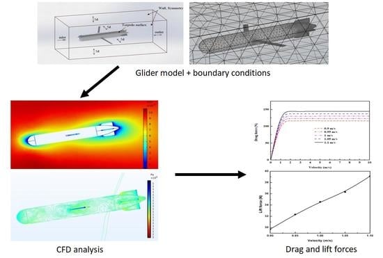
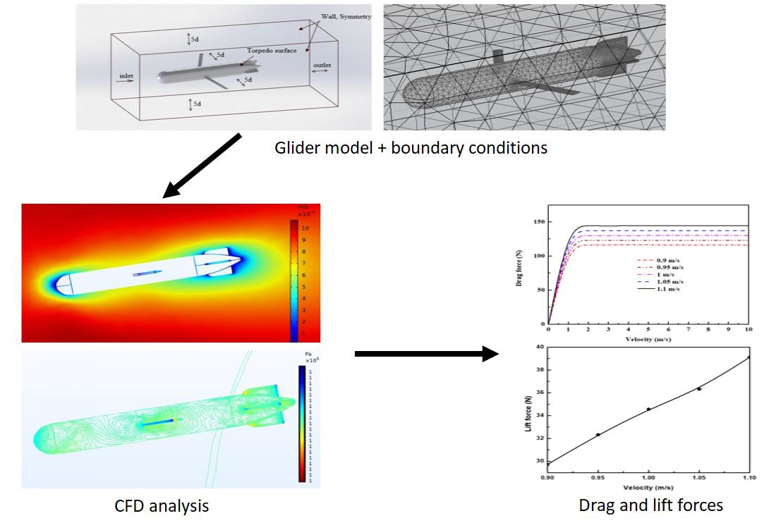
2. Physical Model and Numerical Approach
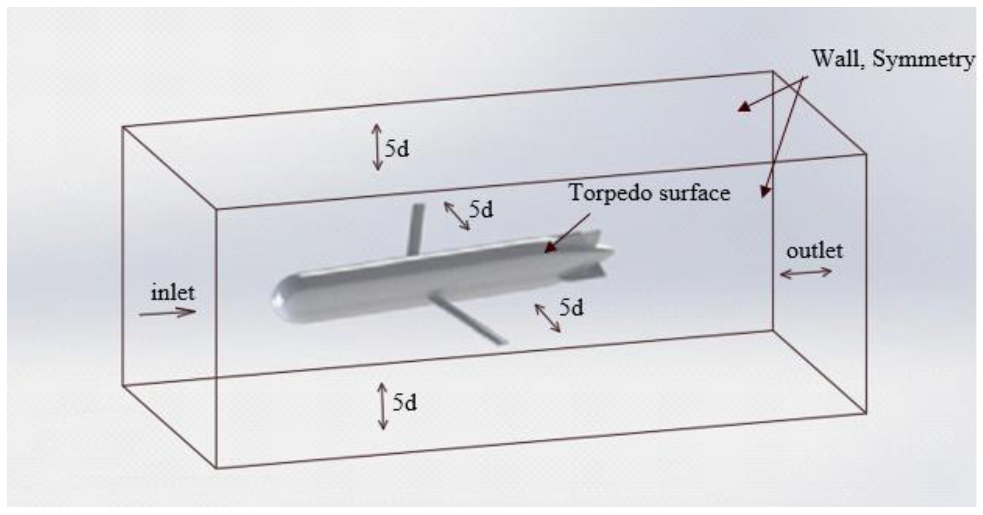
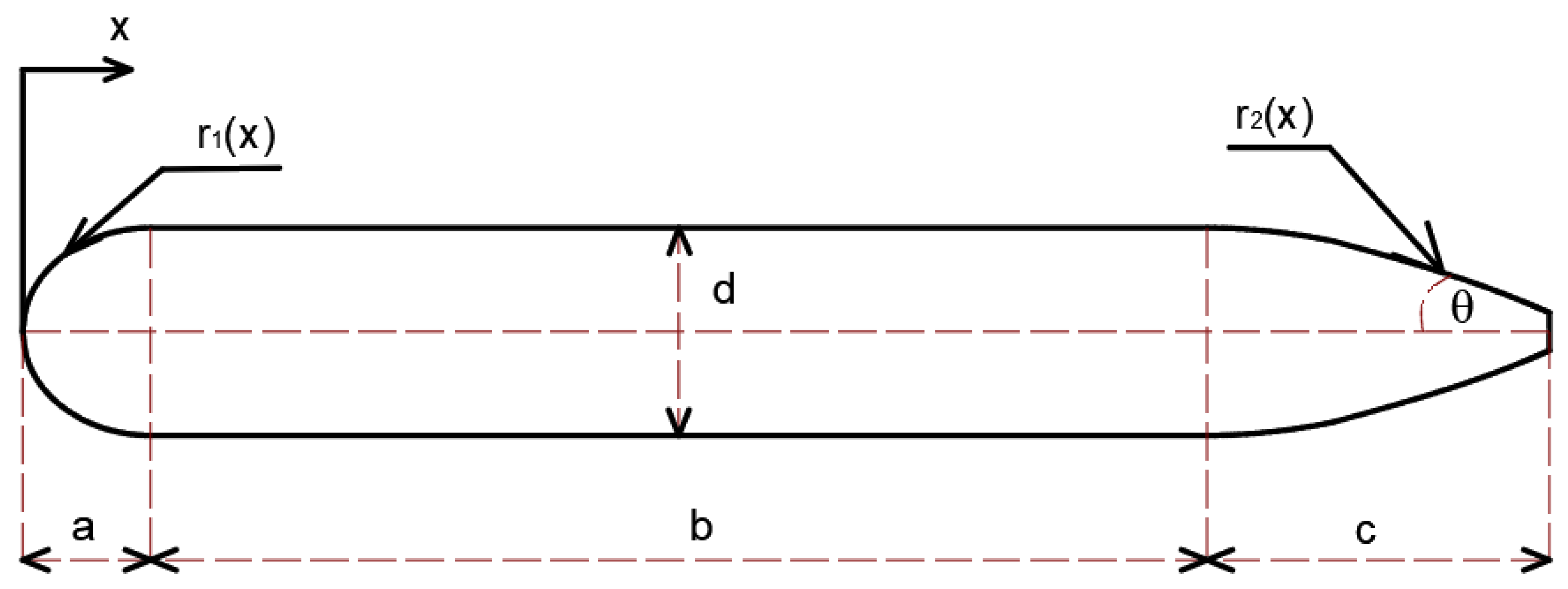
2.1. Physical Model
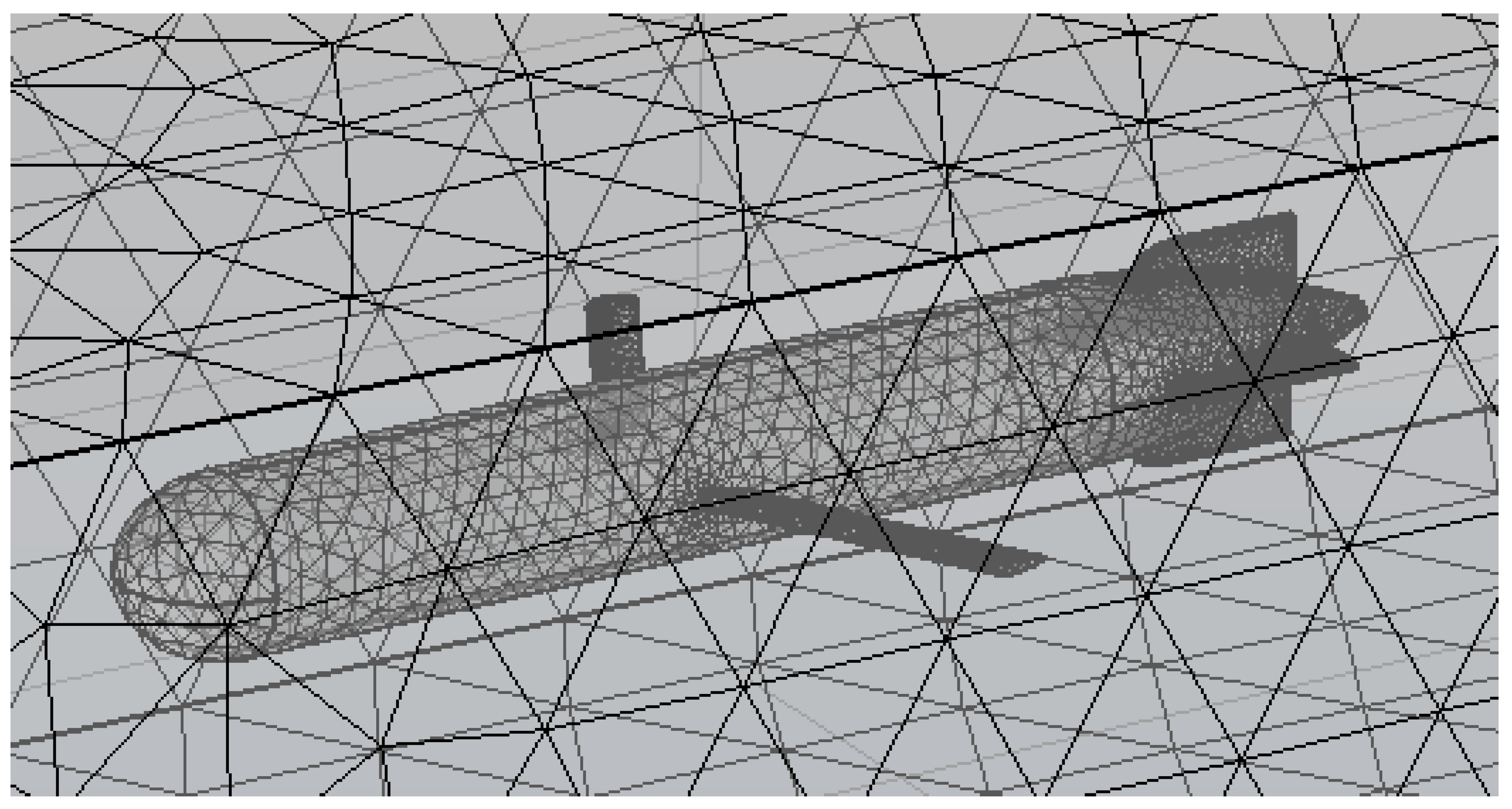
2.2. Numerical Approach
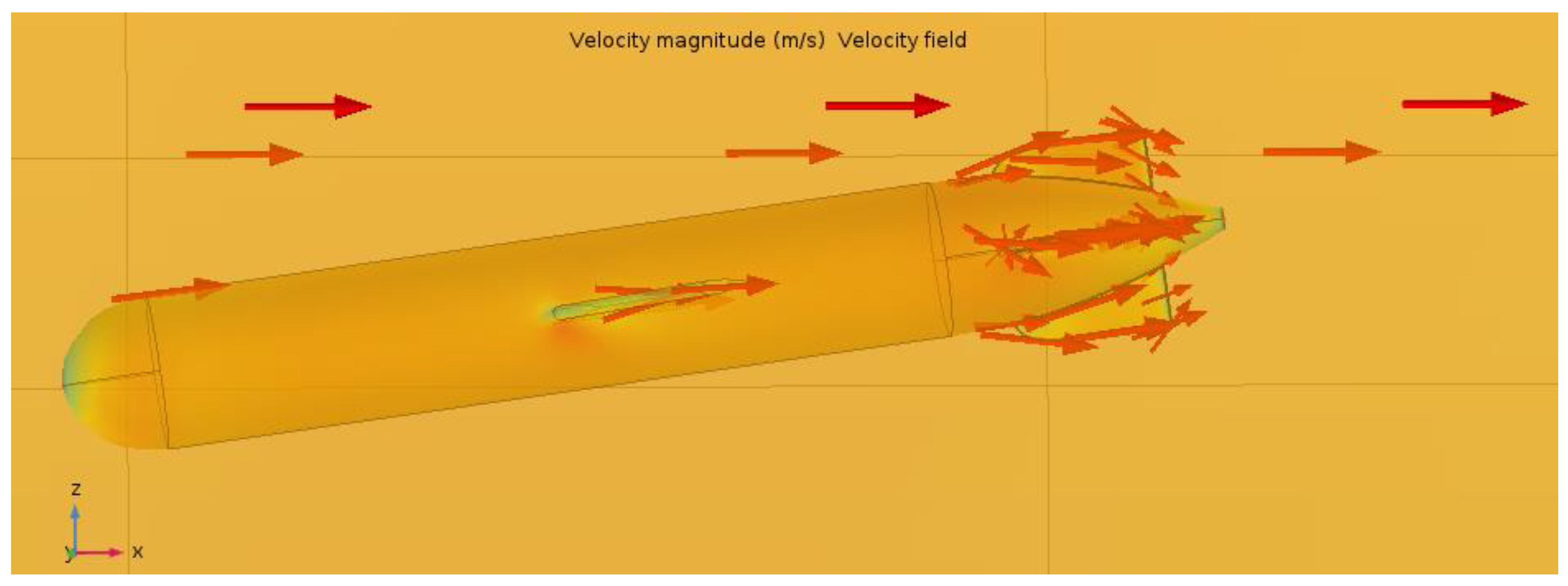
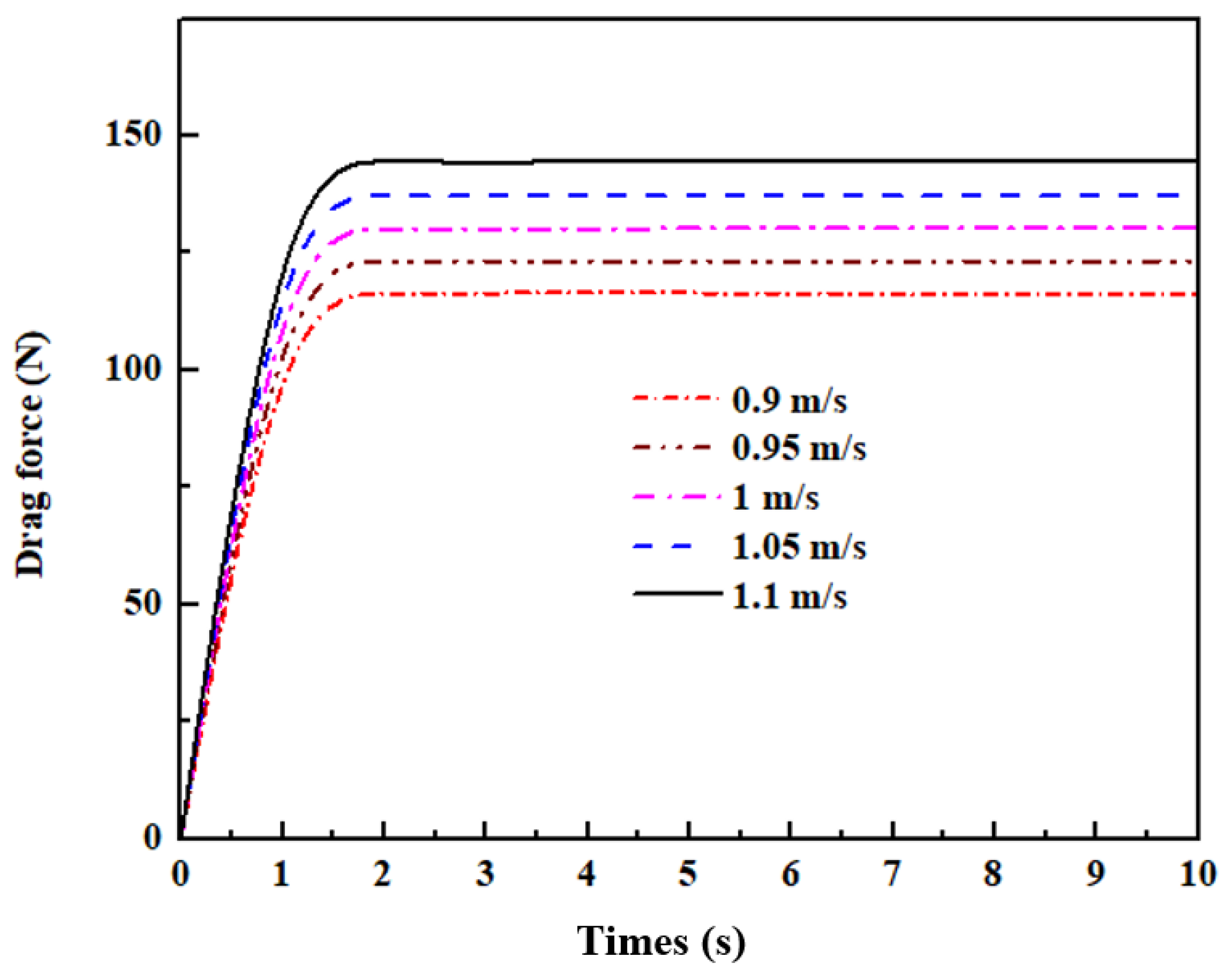
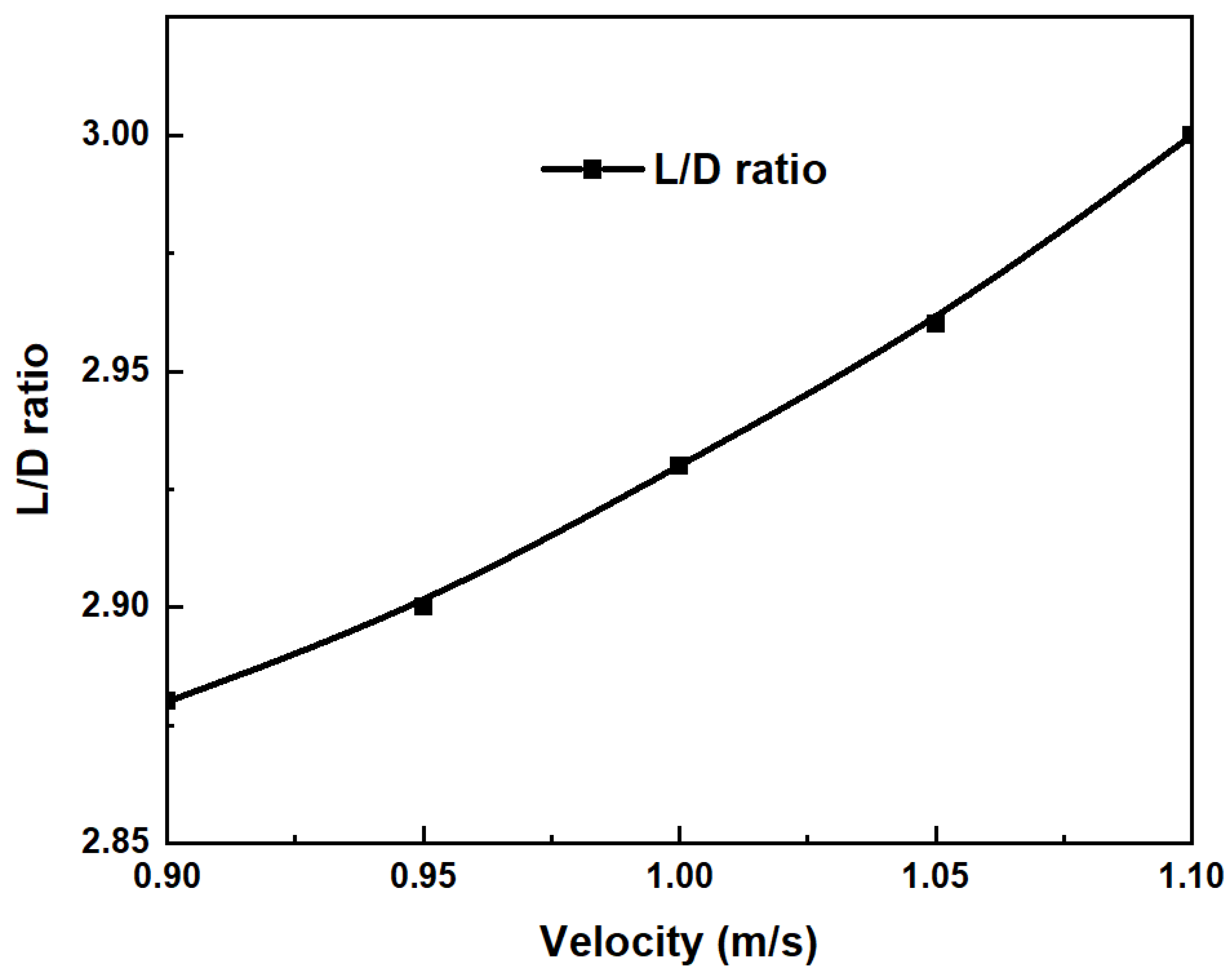
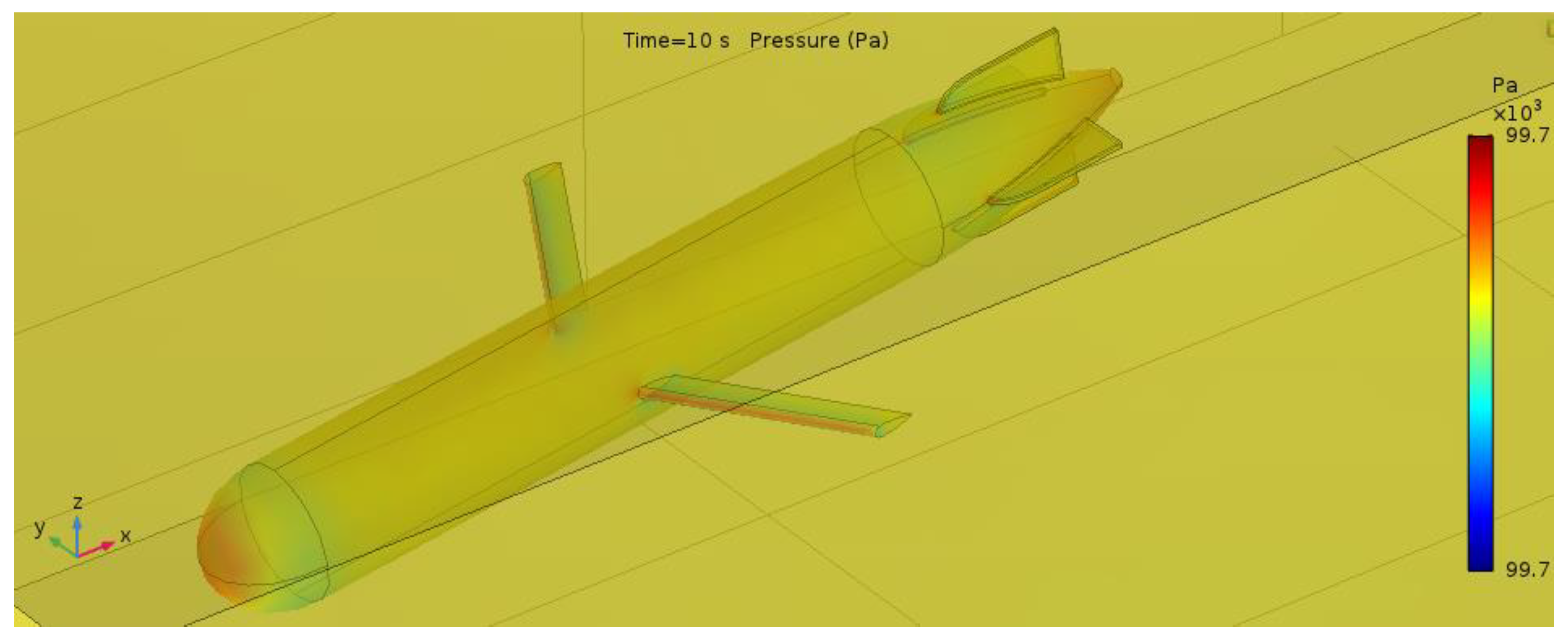
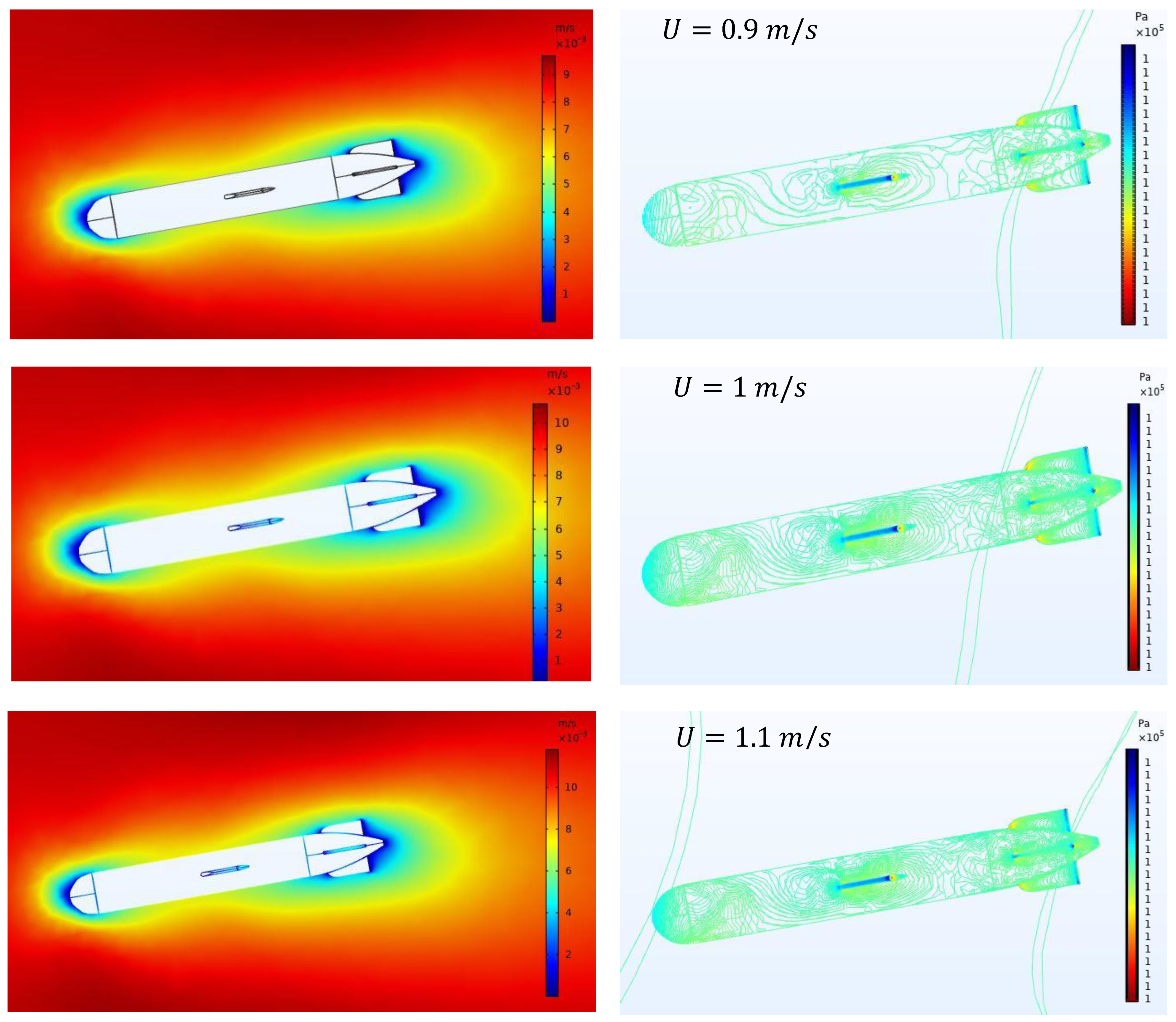
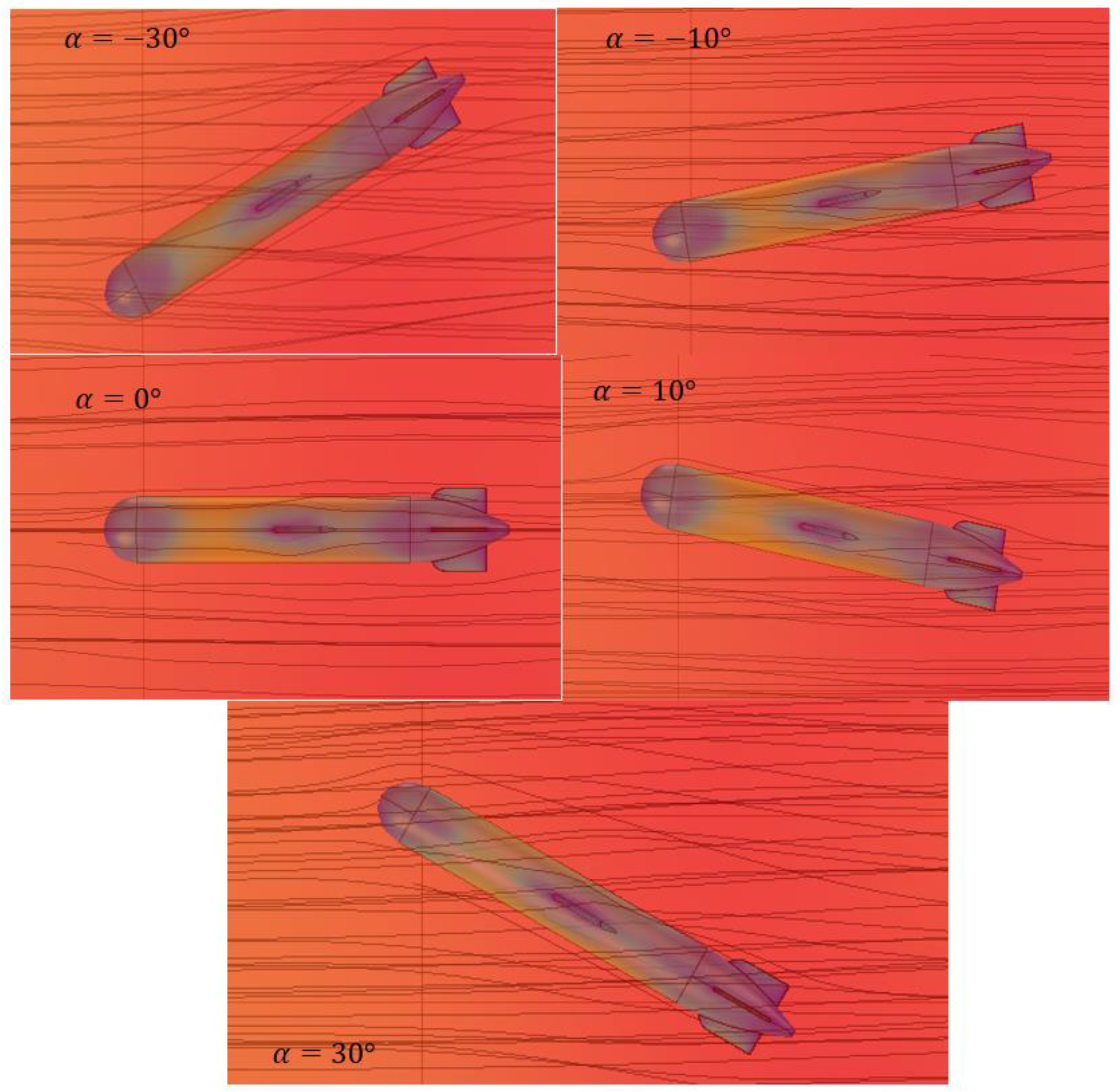
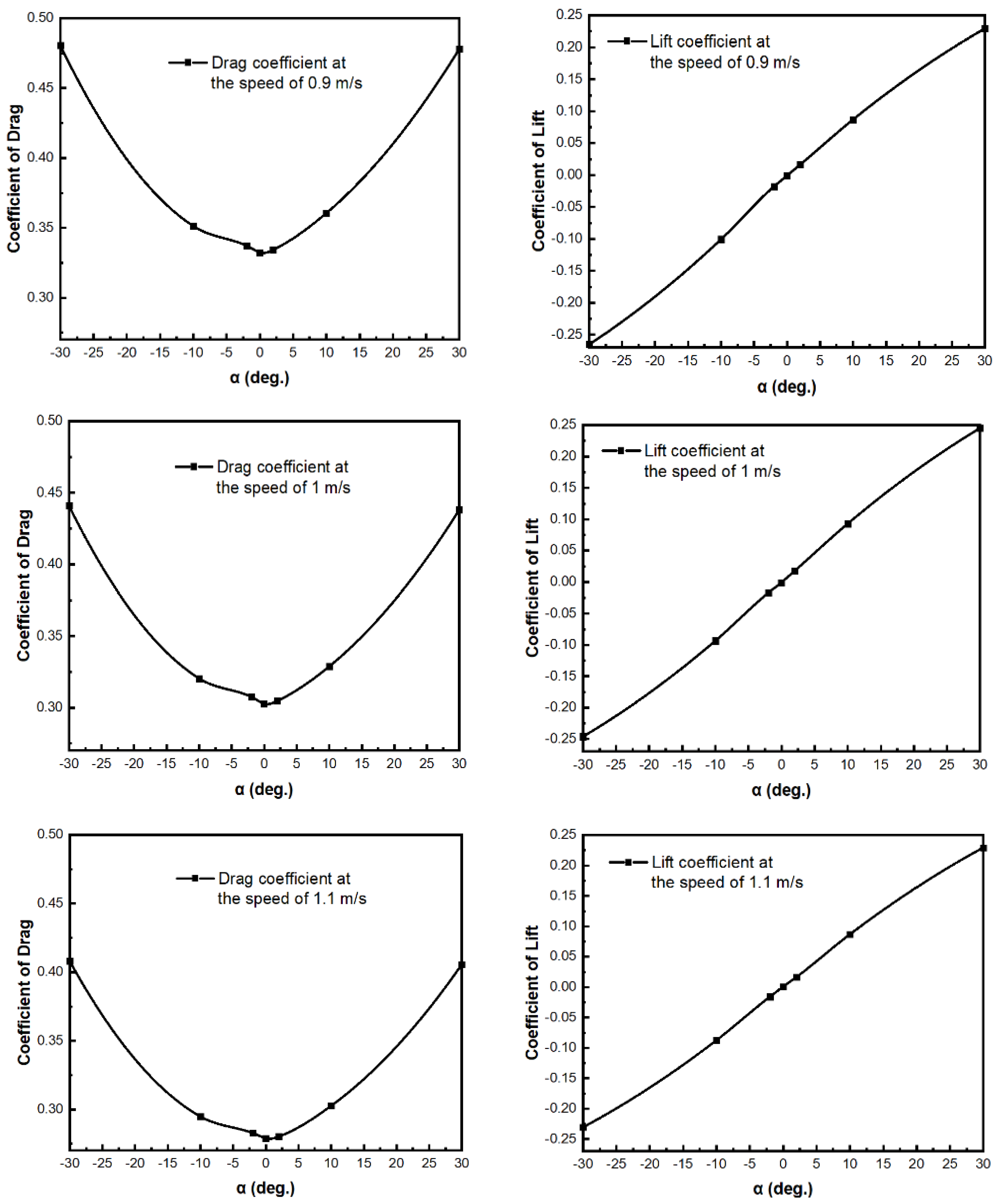
3. Results and Discussion
4. Concluding Remarks
Author Contributions
Funding
Acknowledgments
Conflicts of Interest
References
- Lurton, X. An Introduction to Underwater Acoustics: Principles and Applications; Springer: Berlin/Heidelberg, Germany, 2010. [Google Scholar]
- Leonard, J.J.; Bahr, A. Autonomous Underwater Vehicle Navigation. In Springer Handbook of Ocean Engineering; Springer: Berlin/Heidelberg, Germany, 2016; pp. 341–358. [Google Scholar]
- Niu, H.; Adams, S.; Lee, K.; Husain, T.; Bose, N. Applications of Autonomous Underwater Vehicles in Offshore Petroleum Industry Environmental Effects Monitoring. J. Can. Pet. Technol. 2009, 48, 12–16. [Google Scholar] [CrossRef]
- Cui, W. An Overview of Submersible Research and Development in China. J. Mar. Sci. Appl. 2018, 17, 459–470. [Google Scholar] [CrossRef]
- Sahoo, A.; Dwivedy, S.K.; Robi, P. Advancements in the field of autonomous underwater vehicle. Ocean. Eng. 2019, 181, 145–160. [Google Scholar] [CrossRef]
- Amiri, M.M.; Sphaier, S.H.; Vitola, M.A.; Esperana, P.T. URANS investigation of the interaction between the free surface and shallowly submerged underwater vehicle at steady drift. Appl. Ocean Res. 2019, 84, 192–205. [Google Scholar] [CrossRef]
- Myring, D.F. A Theoretical Study of Body Drag in Subcritical Axisymmetric Flow. Aeronaut. Q. 1976, 27, 186–194. [Google Scholar] [CrossRef]
- Mitra, A.; Panda, J.; Warrior, H. Experimental and numerical investigation of the hydrodynamic characteristics of Autono-mous Underwater Vehicles over sea-beds with complex topography. Ocean. Eng. 2020, 198. [Google Scholar] [CrossRef] [Green Version]
- Yu, P.; Wang, T.; Zhou, H.; Shen, C. Dynamic modelling and three-dimensional motion simulation of a disk type underwater glider. Int. J. Naval Arch. Ocean Eng. 2018, 10, 318–328. [Google Scholar] [CrossRef]
- Ziaeefard, S.; Page, B.R.; Pinar, A.J.; Mahmoudian, N. Effective turning motion control of internally actuated autonomous underwater vehicles. J. Intell. Robot. Syst. 2018, 89, 175–189. [Google Scholar] [CrossRef] [Green Version]
- Singh, Y.; Bhattacharyya, S.K.; Idichandy, V.G. CFD approach to modelling, hydrodynamic analysis and motion charac-teristisc of a laboratory underwater glider with experimental results. J. Ocean Eng. Sci. 2017, 2, 90–119. [Google Scholar] [CrossRef]
- Le, T.-L.; Chen, J.-C.; Shen, B.-C.; Hwu, F.-S.; Nguyen, H.B. Numerical investigation of the thermocapillary actuation behav-ior of a droplet in a microchannel. Int. J. Heat Mass Transf. 2015, 83, 721–730. [Google Scholar] [CrossRef]
- Le, T.-L.; Chen, J.-C.; Hwu, F.-S.; Nguyen, H.B. Numerical study of the migration of a silicone plug inside a capillary tube subjected to an unsteady wall temperature gradient. Int. J. Heat Mass Transf. 2016, 97, 439–449. [Google Scholar] [CrossRef]
- Le, T.-L.; Chen, J.-C.; Nguyen, H.B. Numerical study of the thermocapillary droplet migration in a microchannel under a blocking effect from the heated upper wall. Appl. Therm. Eng. 2017, 122, 820–830. [Google Scholar] [CrossRef]
- Le, T.-L.; Chen, J.-C.; Nguyen, H.-B. Numerical investigation of the forward and backward thermocapillary motion of a wa-ter droplet in a microchannel by two periodically activated heat sources. Numer. Heat Trans. Part A Appl. 2020, 79, 146–162. [Google Scholar] [CrossRef]
- Le, T.-L.; Tien, N.T. A CFD study on hydraulic and disinfection efficiencies of the body sterilization chamber. Ann. Roman. Soc. Cell Biol. 2021, 25, 3998–4004. [Google Scholar]
- Jia, L.J.; Qi, Z.F.; Zhang, S.; Qin, Y.F.; Shi, J.; Zhang, X.M.; Sun, X.J. Dynamic Analysis of the Acoustic Velocity Profile Obser-vation Underwater Glider. Appl. Mech. Mater. 2013, 475, 50–54. [Google Scholar] [CrossRef]
- Guang, P.; Hu, B.; Du, X.X.; Wang, Y.Y.; Pan, G. Research on Hydrodynamic Characteristics of Underwater Gliding UUV Based on the CFD Technique. Adv. Mater. Res. 2012, 479, 729–732. [Google Scholar] [CrossRef]
- Amory, A.; Maehle, E. Modelling and CFD Simulation of a Micro Autonomous Underwater Vehicle SEMBIO. In Proceedings of the OCEANS 2018 MTS/IEEE Charleston, Charleston, SC, USA, 22–25 October 2018. [Google Scholar]
- De Sousa, J.V.N.; de Macêdo, A.R.L.; de Amorim, W.F., Jr.; de Lima, A.G.B. Numerical analysis of turbulent fluid flow and drag coefficient for optimizing the AUV hull design. J. Fluid Dyn. 2014, 4, 263–277. [Google Scholar]
- Randeni, P.S.A.T.; Leong, Z.Q.; Ranmuthugala, D.; Forrest, A.; Duffy, J. Numerical investigation of the hydrodynamic inter-action between two underwater bodies in relative motion. Appl. Ocean. Res. 2015, 51, 14–24. [Google Scholar] [CrossRef]
- Dantas, J.; de Barros, E. Numerical analysis of control surface effects on AUV manoeuvrability. Appl. Ocean. Res. 2013, 42, 168–181. [Google Scholar] [CrossRef]
- Huang, H.; Zhou, Z.; Li, J.; Tang, Q.; Zhang, W.; Gang, W. Investigation on the mechanical design and manipulation hydro-dynamics for a small sized, single body and streamlined I-AUV. Ocean Eng. 2019, 186, 106106. [Google Scholar]
- Mansoorzadeh, S.; Javanmard, E. An investigation of free surface effects on drag and lift coefficients of an autonomous un-derwater vehicle (AUV) using computational and experimental fluid dynamics methods. J. Fluids Struct. 2014, 51, 161–171. [Google Scholar] [CrossRef]
- Cook, G.; Zhang, F. Mobile Robots: Navigation, Control and Sensing, Surface Robots and AUVs; Wiley: Hoboken, NJ, USA, 2020. [Google Scholar]
- Sarkar, T.; Sayer, P.G.; Fraser, S.M. A study of autonomous underwater vehicle hull forms using computational fluid dynam-ics. Int. J. Numer. Methods Fluids 1998, 25, 1301–1313. [Google Scholar] [CrossRef]
- Tyagi, A.; Sen, D. Calculation of transverse hydrodynamic coefficients using compuational fluid dynamic approach. Ocean Eng. 2006, 33, 798–809. [Google Scholar] [CrossRef]
- Jagadeesh, P.; Murali, K.; Jagadeesh, P.; Murali, K. Application of low-Re turbulence models for flow simulations past un-derwater vehicle hull forms. J. Nav. Arch. Mar. Eng. 1970, 2, 41–54. [Google Scholar] [CrossRef] [Green Version]
- Sakthivel, R.; Vengadesan, S.; Bhattacharyya, S. Application of non-linear k-ε turbulence model in flow simulation over un-derwater axisymmetric hull at higher angle of attack. J. Naval Arch. Mar. Eng. 2011, 8, 149–163. [Google Scholar] [CrossRef]
- Panda, J.P.; Warrior, H.V. A Representation Theory-Based Model for the Rapid Pressure Strain Correlation of Turbulence. J. Fluids Eng. 2018, 140. [Google Scholar] [CrossRef]
- Panda, J.; Warrior, H.; Maity, S.; Mitra, A.; Sasmal, K. An improved model including length scale anisotropy for the pres-sure strain correlation of turbulence. ASME J. Fluids Eng. 2017, 139, 44503. [Google Scholar] [CrossRef]
- Panda, J.; Mitra, A.; Joshi, A.; Warrior, H. Experimental and numerical analysis of grid generated turbulence with and with-out mean strain. Exp. Therm. Fluid Sci. 2018, 98, 594–603. [Google Scholar] [CrossRef] [Green Version]
- Mishra, A.A.; Girimaji, S. Linear analysis of non-local physics in homogeneous turbulent flows. Phys. Fluids 2019, 31, 35102. [Google Scholar] [CrossRef]
- Mishra, A.A.; Girimaji, S.S. Pressure–Strain Correlation Modeling: Towards Achieving Consistency with Rapid Distortion Theory. Flow Turbul. Combust. 2010, 85, 593–619. [Google Scholar] [CrossRef]
- Mishra, A.A.; Girimaji, S.S. Intercomponent energy transfer in incompressible homogeneous turbulence: Multi-point physics and amenability to one-point closures. J. Fluid Mech. 2013, 731, 639–681. [Google Scholar] [CrossRef]
- Mishra, A.A.; Girimaji, S.S. On the realizability of pressure-strain closures. J. Fluid Mech. 2014, 755, 535–560. [Google Scholar] [CrossRef]
- Mishra, A.A.; Girimaji, S.S. Hydrodynamic stability of three-dimensional homogeneous flow topologies. Phys. Rev. E 2015, 92, 53001. [Google Scholar] [CrossRef] [PubMed]
- Mishra, A.A.; Girimaji, S.S. Toward approximating non-local dynamics in single-point pressure-strain correlation closures. J. Fluid Mech. 2017, 811, 168–188. [Google Scholar] [CrossRef]
- COMSOL. COMSOL Multiphysics User’s Guide; COMSOL Inc.: Stockholm, Sweden, 2020. [Google Scholar]
- Joseph, A. Measuring Ocean Currents; Elsevier: Amsterdam, The Netherlands, 2014. [Google Scholar]
- Marsh, R.; Sebille, E.V. Ocean Currents; Elsevier: Amsterdam, The Netherlands, 2021. [Google Scholar]
- Brown, J. Ocean Circulation; Butterworth-Heinemann: Oxford, UK, 1989. [Google Scholar]
- Anton, A.; Cretu, V.; Ruprecht, A.; Muntean, S. Traffic replay compression (TRC): A highly efficient method for handling parallel numerical simulation data. Proc. Rom. Acad. 2013, 14, 385–392. [Google Scholar]


| Parameter | Value |
|---|---|
| a (mm) | 200 |
| b (mm) | 1650 |
| c (mm) | 600 |
| d (mm) | 324 |
| θ (°) | 25 |
| Boundary | Condition |
|---|---|
| Inlet | Prescribed velocity |
| Wall | Pressure on the depth of 100 m |
| Torpedo surface | No-slip |
| Outlet | Pressure on the depth of 100 m |
| Symmetry plane | Symmetry |
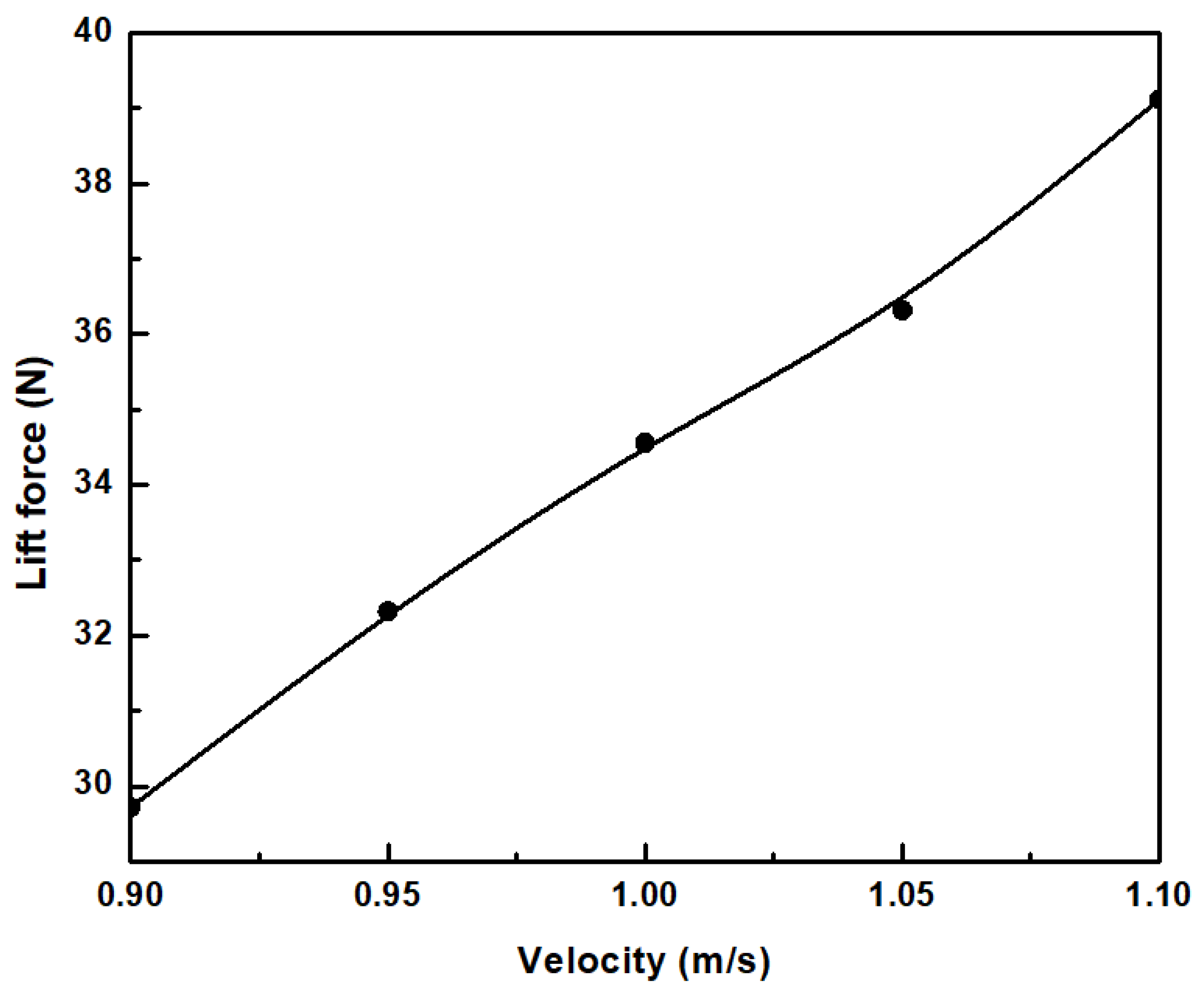
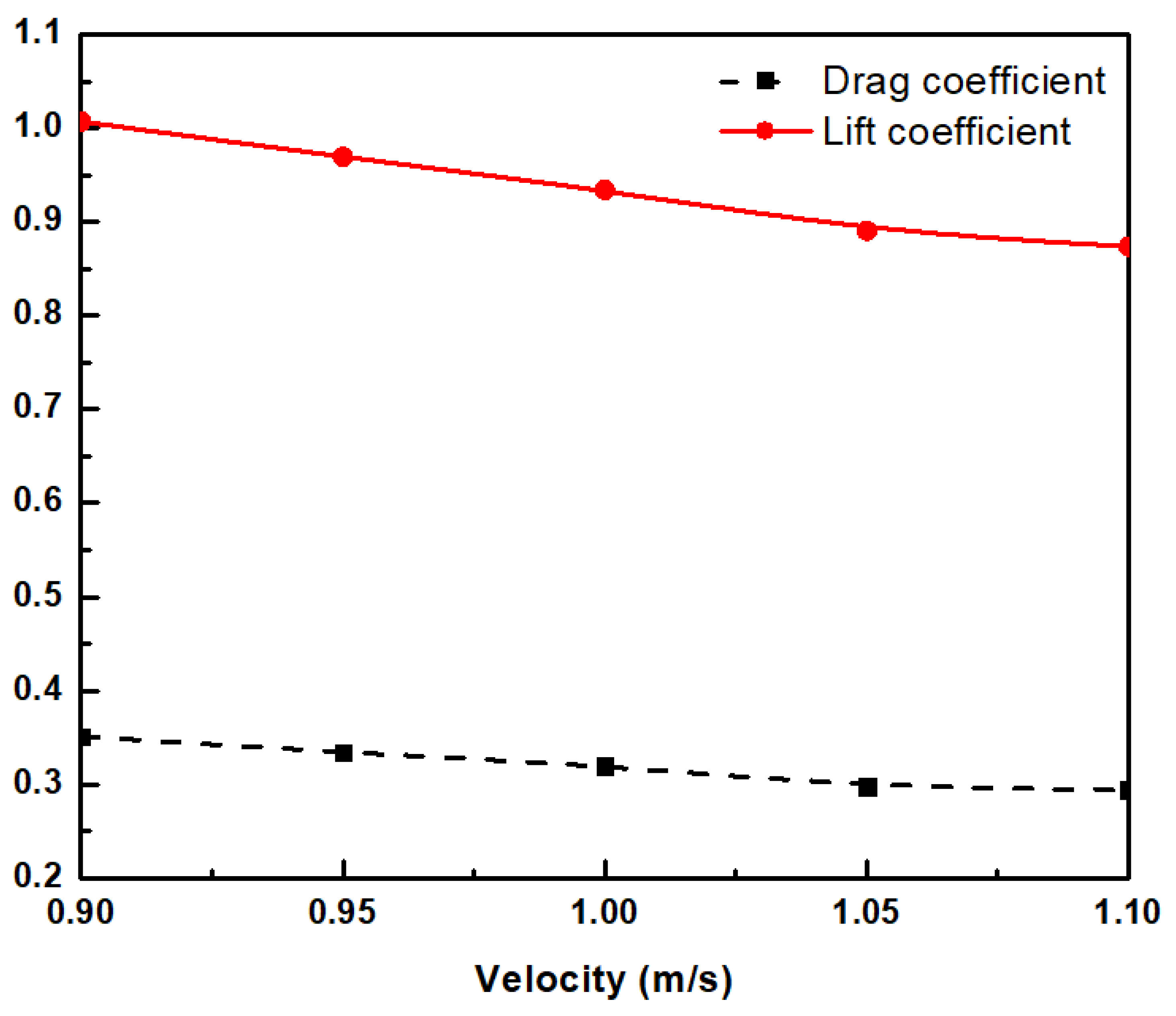
| Velocity (m/s) | Drag Force (N) | Lift Force (N) | Drag Coefficient | Lift Coefficient |
|---|---|---|---|---|
| 0.9 | 105.30 | 30.19 | 0.35 | 1.01 |
| 0.95 | 111.80 | 32.37 | 0.33 | 0.96 |
| 1 | 118.57 | 34.58 | 0.32 | 0.94 |
| 1.05 | 121.20 | 36.33 | 0.30 | 0.89 |
| 1.1 | 127.39 | 39.11 | 0.29 | 0.87 |
Publisher’s Note: MDPI stays neutral with regard to jurisdictional claims in published maps and institutional affiliations. |
© 2021 by the authors. Licensee MDPI, Basel, Switzerland. This article is an open access article distributed under the terms and conditions of the Creative Commons Attribution (CC BY) license (https://creativecommons.org/licenses/by/4.0/).
Share and Cite
Le, T.-L.; Hong, D.-T. Computational Fluid Dynamics Study of the Hydrodynamic Characteristics of a Torpedo-Shaped Underwater Glider. Fluids 2021, 6, 252. https://doi.org/10.3390/fluids6070252
Le T-L, Hong D-T. Computational Fluid Dynamics Study of the Hydrodynamic Characteristics of a Torpedo-Shaped Underwater Glider. Fluids. 2021; 6(7):252. https://doi.org/10.3390/fluids6070252
Chicago/Turabian StyleLe, Thanh-Long, and Duc-Thong Hong. 2021. "Computational Fluid Dynamics Study of the Hydrodynamic Characteristics of a Torpedo-Shaped Underwater Glider" Fluids 6, no. 7: 252. https://doi.org/10.3390/fluids6070252
APA StyleLe, T.-L., & Hong, D.-T. (2021). Computational Fluid Dynamics Study of the Hydrodynamic Characteristics of a Torpedo-Shaped Underwater Glider. Fluids, 6(7), 252. https://doi.org/10.3390/fluids6070252