Migration and Alignment of Three Interacting Particles in Poiseuille Flow of Giesekus Fluids

Abstract

Effect of rheological property on the migration and alignment of three interacting particles in Poiseuille flow of Giesekus fluids is studied with the direct-forcing fictitious domain method for the Weissenberg number (Wi) ranging from 0.1 to 1.5, the mobility parameter ranging from 0.1 to 0.7, the ratio of particle diameter to channel height ranging from 0.2 to 0.4, the ratio of the solvent viscosity to the total viscosity being 0.3 and the initial distance (y₀) of particles from the centerline ranging from 0 to 0.2. The results showed that the effect of y₀ on the migration and alignment of particles is significant. The variation of off-centerline (y₀ ≠ 0) particle spacing is completely different from that of on-centerline (y₀ = 0) particle spacing. As the initial vertical distance y₀ increased, the various types of particle spacing are more diversified. For the off-centerline particle, the change of particle spacing is mainly concentrated in the process of cross-flow migration. Additionally, the polymer extension is proportional to both the Weissenberg number and confinement ratio. The bigger the Wi and confinement ratio is, the bigger the increment of spacing is. The memory of shear-thinning is responsible for the reduction of d₁. Furthermore, the particles migrate abnormally due to the interparticle interaction.

1. Introduction

Particle migration in Newtonian or non-Newtonian fluids has been extensively studied due to the wide-ranging applied background in scientific and industrial fields, such as particle separation, focusing and sorting [1,2,3]. In many of these devices, such as flow cytometers [4,5] and continuous-flow sorters [6,7], focusing particles into a train is a necessary step prior to sorting and detecting them. Specifically, blood cell analysis by flow cytometry is routinely applied for therapy control and medical diagnostics in immunology and hematology [8]. The most important advantage of flow cytometry is the high frequency at which cells are differentiated and counted. Cells are differentiated by measuring light scatter in an orthogonal or forward direction. Mastering the variation of particle spacing is beneficial for improving the efficiency of particle sorting and cell detection. Therefore, understanding the migration and equilibrium pattern of particles in the fluids could provide a theoretical basis for particle manipulation.

The first observation of the cross-flow migration of particles in a pressure-driven pipe flow of Newtonian fluid was made by Segré and Silberberg [9]. The experimental results indicated that the particles were collected into a thin annulus at about 0.6 times the tube radii from the axis. Afterward, much work has been done to investigate the cross-flow migration of particles in a pressure-driven flow of Newtonian fluid. Compared to the particle migration toward the equilibrium position in Newtonian fluid, the particles would migrate to the centerline [10,11] or the closest wall in a non-Newtonian fluid [12], in which the particle migration is dependent on the competition between fluid inertia, elasticity, shear-thinning and geometric confinement [13]. Specifically, the elasticity makes particles migrate to the centerline, whereas the shear-thinning and geometric confinement drive particles toward the closest wall. There existed a boundary between the wall and the centerline, and the particles between the centerline and boundary would migrate toward the centerline, otherwise, particles would migrate toward the closest wall. The position of the boundary is determined by the above factors. The neutrally buoyant cylinder’s migration in viscoelastic fluids and the intrinsic mechanism are investigated in numerical simulations [14]. In Poiseuille flow with the limit of negligible inertia, the migration of particles is controlled by elastic normal stresses, which are compressive and proportional to the square of the shear rate. If the blockage is strong, the effect of elastic normal stresses is manifested by an attraction toward the nearby wall. If the blockage is weak, the normal stresses act through the curvature of the inflow velocity profile and generate a lateral force that points to the centerline. Additionally, there is a different phenomenon when particles migrate in the channel with a rectangular cross-section, i.e., particles would move to the corners due to the existence of the secondary flows [15,16].

Comparing with the cross-flow migration of a single particle in fluid, the migration behavior of multi-particles caused by the particle-particle interaction in a non-Newtonian fluid is more peculiar and more diverse. For the particle-particle interaction in the shear flow, there existed three patterns in the Oldroyd-B fluid, i.e., returning, tumbling and passing, while the tumbling behavior was not found in a shear-thinning viscoelastic polymer solution [17]. This suggested that tumbling may be related to the elasticity but not the shear-thinning property. Which pattern appears strongly dependent on the initial distance of the particle from the centerline. There was a separatrix between the returning and passing pattern. When the initial position is above the critical distance corresponding to the separatrix, the particles pass each other. Otherwise, the particles move toward a stable position on the centerline after they return. The returning/passing separatrix position depended on the Weissenbrg number, shear-thinning property and geometric confinement.

Another migration behavior of multi-particles in a non-Newtonian fluid is the particle alignment in the shear flow. The particle-particle interaction becomes more significant as the distance between particles decreases. The earlier experimental results showed that the particles lined up in the flow direction and formed a chain structure [18]. Choi et al. [19] presented a numerical algorithm to cope with the movement of particles. The results revealed the impact of the Weissenberg number, geometric confinement and viscosity ratio on the formation of chain-like structures. Xiang et al. [20] experimentally explored that, in a viscoelastic fluid where the inertia effect was comparable with the elastic effect, particles equilibrate at two symmetrical positions in the centerline, and a third focusing position at the center with further increase in the flow rate. Pasquino et al. [21] performed experiments and showed that the occurrence of particle migration had a non-negligible effect on the formation of a particle string in the shear flow. Pan et al. [22] observed the long-lived trains of particles aligned with the flow at high particle concentration in an experimental study. D’Avino et al. [23] studied the dynamics of pairs and triplets of particles by numerical simulations, and the results showed that, for the case of three particles, when the Deborah number was less than the critical De, the particles would separate if the interparticle distance between the leftmost and the middle one and the interparticle distance between the rightmost and the middle one were all larger than the critical distance, and otherwise the leftmost particle and the middle particle formed a pair and the rightmost particle separated.

As is shown above, there is still some work to be done in the study of the interaction and alignment of multiple particles when the particles are not initially located on the centerline. The former study [23] has proved that cross-flow migration has an important impact on string formation. In the present study, we investigate numerically the interaction among three neutrally buoyant and equally sized particles that are not initially located on the centerline in a Poiseuille flow of Giesekus fluids and focus on the effect of the initial distance of particles from the centerline, shear-thinning property, Weissenberg number and wall confinement on the behavior of migration and alignment of three interacting particles. In order to investigate the sole effect of fluid viscoelasticity, both fluid and particle inertia is neglected.

2. Numerical Model

2.1. Fictitious Domain Method

The direct-forcing fictitious domain (DF-FD) method is used to simulate particle migration. The DF-FD method is an improved version of the earlier distributed-Lagrange-multiplier/fictitious domain (DLM/FD) method, which was initially developed by Glowinski et al. [24] to solve the particle differential equations. The key idea of the DLM/FD is that the interior of the particle is filled with fluid, and a pseudo body force is exerted over the particle inner domain to enforce the fictitious fluid to satisfy the rigid-body motion constraint. More details about the DF/FD approach could be referred to in reference [25]. Here the solid domain and the entire domain, including both the interior and exterior of the solid body, are denoted by P(t) and Ω, respectively. In the FD method, the following scales are introduced to achieve nondimensionalization: H for length, U₀ for velocity, H/U₀ for time, ${\rho }_f{\mathit{u}}_0^2$ for pressure and ${\rho }_f{\mathit{u}}_0^2/H$for pseudo body-force. The dimensionless basic equations in the DF-FD method are as follows:

(i) Combined momentum equations:

$$\frac{\partial \mathit{u}}{\partial t}+\mathit{u}\cdot \nabla \mathit{u}=\frac{{\eta }_r{\nabla }^2\mathit{u}}{Re}-\nabla p+\frac{\left(1-{\eta }_r\right)\nabla \cdot \mathit{B}}{ReWi}+\lambda , \mathrm{in} \Omega$$

(1)

$$\mathit{u}=\mathit{U}+{\mathbf{\omega }}_p\mathbf{\times }\mathit{r}, \mathrm{in} P\left(t\right)$$

(2)

$$\left({\rho }_r-1\right)V_p^{*}\frac{\mathrm{d}\mathit{U}}{dt}=-{\displaystyle {\int }_P\lambda \mathrm{d}x},$$

(3)

$$\left({\rho }_r-1\right)J^{*}\frac{\mathrm{d}{\mathbf{\omega }}_p}{\mathrm{d}t}=-{\displaystyle {\int }_P\mathit{r}\times \lambda dx}.$$

(4)

(ii) Continuity equation:

$$\nabla \cdot \mathit{u}=0, \mathrm{in} \Omega .$$

(5)

(iii) Constitutive equation of Giesekus fluid:

$$\frac{\partial \mathit{B}}{\partial t}+\mathit{u}\cdot \nabla \mathit{B}-\mathit{B}\cdot \nabla \mathit{u}-{\left(\nabla \mathit{u}\right)}^T\cdot \mathit{B}+\frac{\alpha }{Wi}{\left(\mathit{B}-I\right)}^2+\frac{\mathit{B}-I}{Wi}=0, \mathrm{in} \Omega$$

(6)

In which u, p, and λ are the fluid velocity, pressure and Lagrange multiplier, respectively, and λ is defined in the solid domain P(t); ω_p is the particle angular velocity; ρ_r = ρ_s/ρ_f is the ratio of the particle density ρ_s to the fluid density ρ_f; r is the position vector in respect to the mass center of the particle; Re = ρ_fU₀H/η₀ is the Reynolds number (U₀ and H are the characteristic velocity and length, respectively, η₀ = η_s + η_p is the total zero shear-rate viscosity with η_s and η_p being the solvent and polymer viscosity, respectively); $V_p^{*}=V_p/H^3$ is the dimensionless particle volume; J^* = J/ρ_sH⁵ is the dimensionless moment of inertia; Wi = λ_tU₀/H is the Weissenberg number (λ_t is the fluid relaxation time); B is the polymer configuration tensor that is related to the polymer stress τ = η_p(B−I)/λ_t; α is the mobility parameter and quantifies the entity of the shear-thinning (α = 0 corresponds to the Oldroyd-B fluid without shear-thinning property).

A fractional-step time scheme is used to decouple Equations (1)–(6) into the following three sub-problems.

(i) Fluid sub-problem for ${\mathit{u}}^{*}$ and p:

$$\frac{{\mathit{u}}^{*}-{\mathit{u}}^n}{\Delta t}-\frac{{\eta }_r{\nabla }^2{\mathit{u}}^{*}}{2Re}=-\nabla p+\frac{1}{2}\left[3{\mathit{G}}^n-{\mathit{G}}^{n-1}\right]+\frac{{\eta }_r{\nabla }^2{\mathit{u}}^n}{2Re}+{\lambda }^n,$$

(7)

$$\nabla \cdot {\mathit{u}}^{*}=0,$$

(8)

$$\mathit{G}=-\mathit{u}\cdot \nabla \mathit{u}+(\frac{1-{\eta }_r}{ReWi})\nabla \cdot \mathit{B}.$$

(9)

This sub-problem is virtually the solution of the Navier–Stokes equation. Here a finite, difference-based projection approach on a homogeneous half-staggered grid is employed for spatial discretization, and all spatial derivatives are discretized with the second-order central difference scheme.

(ii) Particle sub-problem for Uⁿ⁺¹, ω_pⁿ⁺¹, λⁿ⁺¹, u ⁿ⁺¹:

$${\rho }_r{V}_p^{*}\frac{{\mathit{U}}^{n+1}}{\Delta t}=\left({\rho }_r-1\right)V_p^{*}\frac{{\mathit{U}}^n}{\Delta t}+{\displaystyle {\int }_P\left(\frac{{\mathit{u}}^{*}}{\Delta t}-{\lambda }^n\right)}dx,$$

(10)

$${\rho }_r\frac{J^{*}{\mathbf{\omega }}_p^{n+1}}{\Delta t}=\left({\rho }_{\mathit{r}}-1\right)\frac{J^{*}{\mathbf{\omega }}_p^n}{\Delta t}+{\displaystyle {\int }_{P}r\times \left(\frac{{\mathit{u}}^{*}}{\Delta t}-{\lambda }^n\right)}dx.$$

(11)

Note that the above equations have been reformulated so that all the terms on the right-hand side of the equations are known and consequently Uⁿ⁺¹ and ${\mathbf{\omega }}_p^{n+1}$ can be obtained without iteration. Then the Lagrange multipliers (λⁿ⁺¹) defined at the Lagrangian nodes can be determined by:

$${\lambda }^{n+1}=\frac{{\mathit{U}}^{n+1}+{\mathbf{\omega }}_p^{n+1}\times \mathit{r}-{\mathit{u}}^{*}}{\Delta t}+{\lambda }^n,$$

(12)

and the fluid velocities (${\mathit{u}}^{n+1}$) defined at the Eulerian nodes are corrected as:

$${\mathit{u}}^{n+1}={\mathit{u}}^n+\Delta t\left({\lambda }^{n+1}-{\lambda }^n\right),$$

(13)

In which u and λ are defined at the Eulerian and Lagrangian nodes, respectively. Consequently, u and λ are transferred from the Eulerian nodes to the Lagrangian nodes and from the Lagrangian nodes to the Eulerian nodes, respectively, using the tri-linear interpolation function. For the spherical particle, the Lagrangian nodes are distributed on a sequence of spherical surfaces.

(iii) Constitutive equation sub-problem for B:

$$\frac{{\mathit{B}}^{n+1}-{\mathit{B}}^n}{\Delta t}+{\mathit{u}}^{n+1}\cdot \nabla {\mathit{B}}^n-{\mathit{B}}^n\cdot \nabla {\mathit{u}}^{n+1}-{\left(\nabla {\mathit{u}}^{n+1}\right)}^T\cdot {\mathit{B}}^n+\frac{\alpha }{Wi}{\left({\mathit{B}}^n-I\right)}^2+\frac{{\mathit{B}}^{n+1}-I}{W\mathrm{i}}=0,$$

(14)

where${\mathit{u}}^{n+1}$ can be determined from the sub-problem (i) and (ii). Equation (14) is solved with the first-order time scheme, the central difference scheme for the velocity gradient and the third-order upwinding MUSCL scheme for the convective term.

The fictitious domain method has been widely used and well-validated [15,16,26,27]. Here we further verify the feasibility of this method by comparing the present results of circular particle lateral trajectory in a Poiseuille flow of Oldroyd-B fluid to those obtained with the finite element method [28] as shown in Figure 1, where η_r = η_s/η₀ and the ratio of the particle diameter to the channel height is d/H. The dimensionless computation domain x × y is 4 × 2, and two grid sizes, h = 1/128 and h = 1/64, are used. The time step Δt = 5 × 10⁻⁴ is employed. We can see that the present results are in good agreement with the previous numerical results, especially for the case of h = 1/128. Therefore, the grid size h = 1/128 is used in the following computations.

2.2. Collision Model

A collision model is used to prevent the mutual penetration of particles when they collide:

$$F_{ij}=F_0\left(1-d_{ij}/d_c\right)n_{ij},$$

(15)

where F_ij, d_ij and n_ij are the repulsive force exerting on particle j by particle i, the distance between two particles and the unit normal vector pointing from the center of particle i to that of particle j, respectively; d_c is a cutoff distance within which the repulsive force is activated and d_c = h (mesh size) here; F₀ = 10³ is the magnitude of the force at contact. Equations (10), (11) and (15) are solved separately with a fractional-step scheme to obtain particle migrations. We set the time step for the collision model to be one-tenth of the latter to circumvent the stiffness problem arising from the explicit integration scheme with a large value of the force F₀ [24].

2.3. Simulation Setup

We are concerned with the dynamics of three neutrally buoyant particles (ρ_r = 1) in a pressure-driven flow of viscoelastic fluid in this work. A Cartesian coordinate system is built up with its origin at the channel inlet, as shown in Figure 2, where the computational domain spans over [0, L] and [−H/2, H/2] in the x and y directions, respectively. The periodic boundary condition is applied in the streamwise direction, and a no-slip boundary condition is imposed at the channel walls and particle surface. Three particles are named particle 1, 2 and 3 from left to the right, respectively. x₁, x₂, x₃ represent the abscissa of particle center (particle 1, 2, 3) and the interparticle distances in the x-direction are defined as d₁ = x₂ − x₁ − d_p and d₂ = x₃ − x₂ − d_p, respectively. The initial interparticle distances in the x-direction are denoted by d_1,0 and d_2,0, and the initial distance of particles from the centerline is represented as y₀. The characteristic velocity U₀ is the velocity at the channel centerline. The confinement ratio ε is defined as ε = d_p/H. We take L = 16H in order to avoid the impact of channel length on the numerical results. The time-step Δt is 5 × 10⁻⁴. Since the inertia is neglected, we set Re = 0.1.

3. Results and Discussion

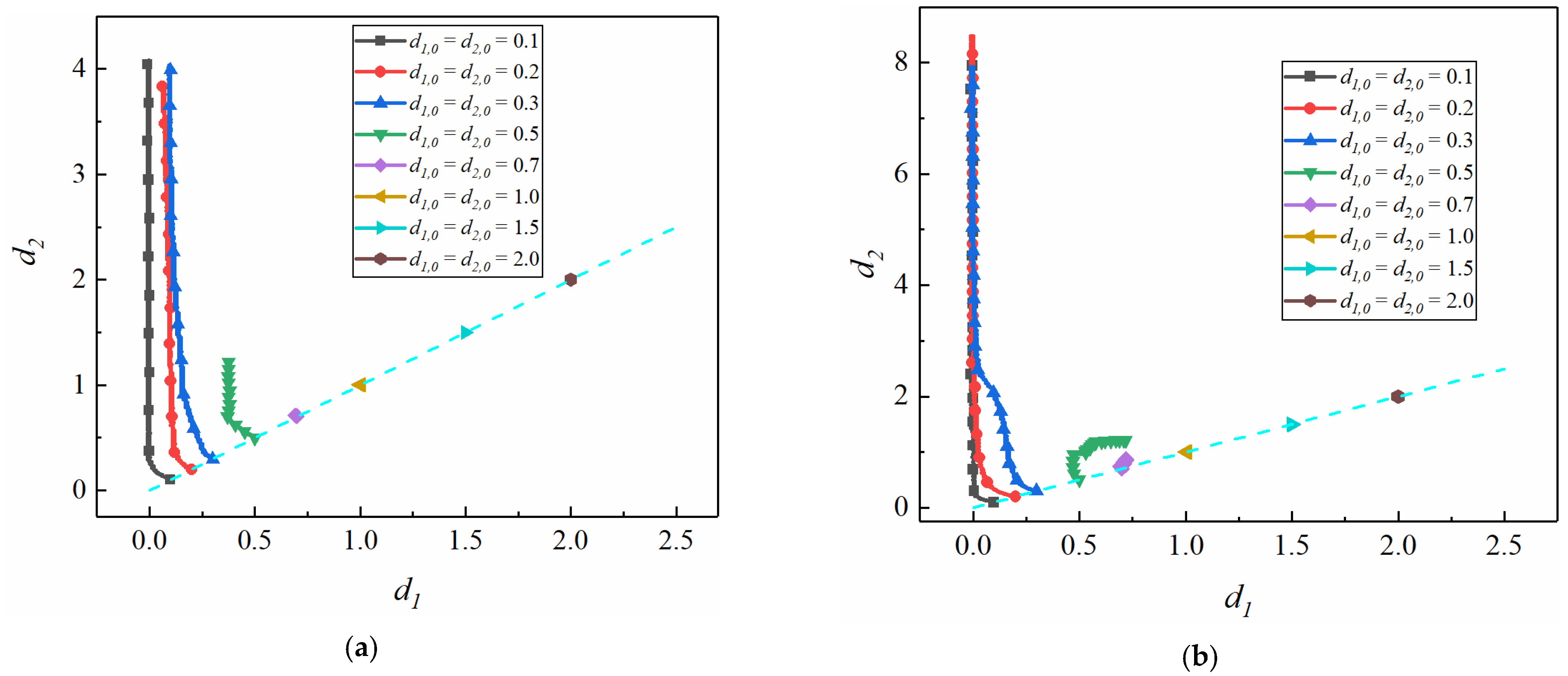
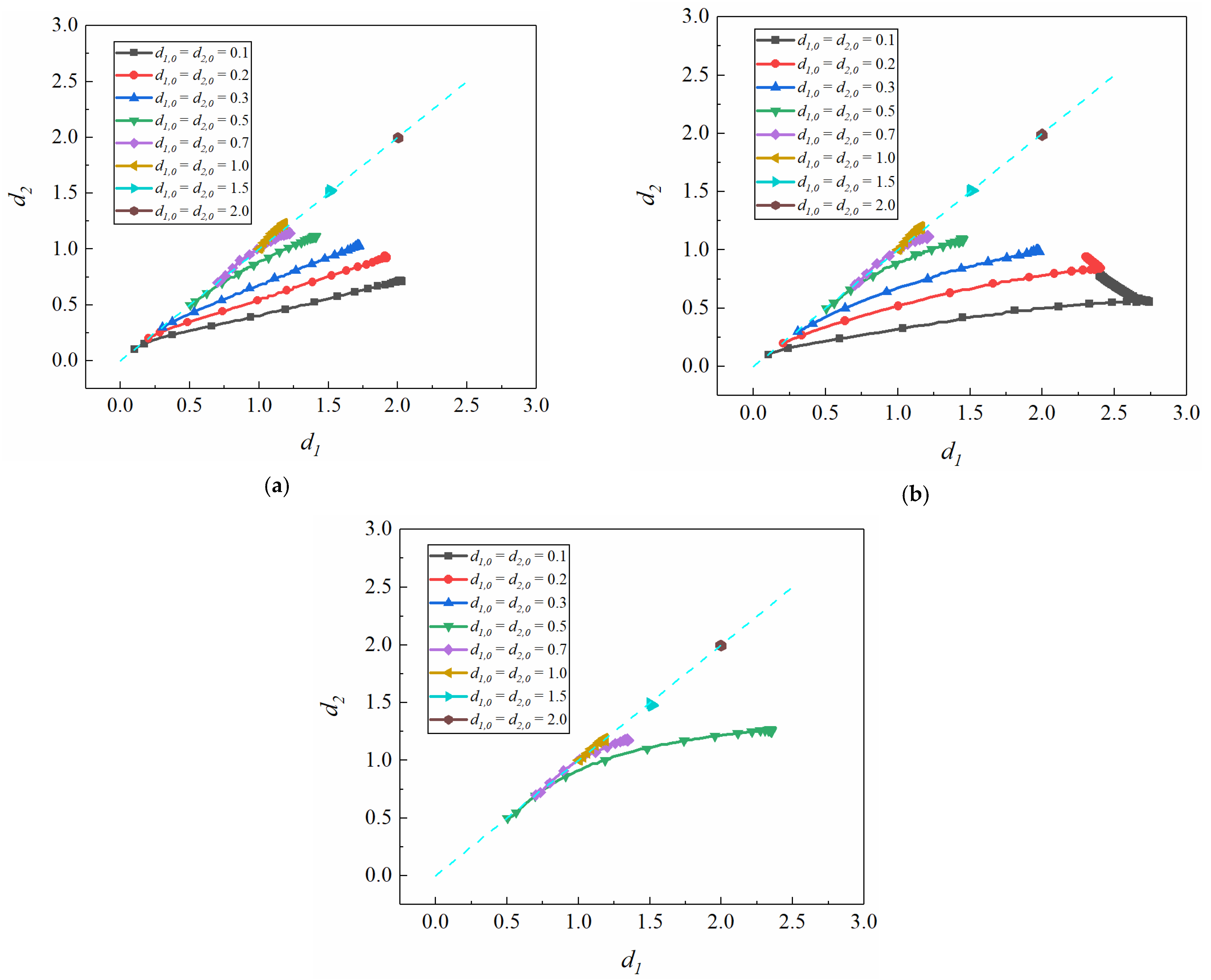
3.1. Effect of Initial Distance from the Centerline on the Interparticle Distance

Three particles are initially located at the same position y₀, as shown in Figure 2. The simulation is ended when the particles travel a length of 2000 times the channel height along the flow direction. Variations of interparticle distances d₁ and d₂ for different initial interparticle spacing d_1,0, d_2,0 are shown in Figure 3, where three particles are initially located on different vertical positions y₀. The variation of interparticle spacing depends on the relationship between the initial interparticle distance and the initial vertical position y₀. For the particle initially located on the channel centerline in Figure 3a, when the initial interparticle distances are small (d_1,0 = d_2,0 = 0.1, 0.2 and 0.3), the interparticle distance d₁ decreases to 0 while d₂ increases continuously, and finally, particle 1 forms a pair with particle 2 while particle 3 is isolated. When the initial interparticle distances are large (d_1,0 = d_2,0 = 1.0, 1.5 and 2.0), there is no interaction among the three particles and the interparticle distances d₁ and d₂ remain unchanged.

When the particles are not initially located on the centerline, they will migrate toward the channel centerline or the wall depending on their initial position from the centerline. In this work, we mainly concentrate on the variation of spacing between particles that migrate to the centerline. Obviously, the variations of the interparticle spacing are affected by the initial vertical positions y₀. In Figure 3b–d, the off-centerline particles migrate toward the centerline, and the variations of interparticle distances are different from those in Figure 3a. Firstly, When the initial interparticle distance d_1,0 = d_2,0 = 0.1, as shown in Figure 3b,c, particle 1 and particle 2 first repel each other and d₁ increases, then d₁ decreases and particle 1 and particle 2 form a pair while particle 3 is isolated. The above process is not observed for y₀ = 0, as shown in Figure 3a. Additionally, in Figure 3a (y₀ = 0), particle 1 and particle 2 form a pair when d_1,0 = d_2,0 = 0.1, 0.2 and 0.3, while the interparticle distance of three particles remains constant when d_1,0 = d_2,0 = 1.0. In Figure 3b (y₀ = 0.1), particle 1 and particle 2 form a pair when d_1,0 = d_2,0 = 0.1 and 0.2, while the three particles repel each other and there is a little increase in the interparticle distance when d_1,0 = d_2,0 = 1.0. In Figure 3c (y₀ = 0.15), particle 1 and particle 2 form a pair only when d_1,0 = d_2,0 = 0.1. While in Figure 3d (y₀ = 0.2), no particle pair is observed, and the interparticle spacing increases along the pathway. The variations of interparticle distances d₁ and d₂ become more obvious for the case of d_1,0 = d_2,0 = 1.0 with increasing y₀. To sum up, the interparticle repulsion increases as the distance (y₀) becomes larger. In Figure 3b–d, the interparticle distances d₁ and d₂ first increase before the particles migrate to the length of 50 H along the flow direction, and then d₁ decreases during the migration process from 50 H to 2000 H.

In order to further explore the effect of y₀ on the particle migration and interparticle distance, we exhibit the variations of interparticle distance under more initial interparticle distances, as shown in Figure 4, where the hollow circles and squares represent the initial configuration. The variation trend of the interparticle distance for y₀ = 0 is shown in Figure 4a, and the results are consistent with the former work [23]. The final configuration is a pair with the interparticle distance tending to be zero and an isolated particle moving far away from the pair. Comparing the variation of particle spacing in Figure 4, the particle migration and interparticle distance are obviously different for y₀ = 0 and y₀ ≠ 0. For y₀ ≠ 0 (y₀ = 0.2), there exists a critical value of initial particle distance, which divides the variation of interparticle distance into two categories. When the initial interparticle distance d_1,0 between particle 1 and particle 2 is small (hollow circle in Figure 4b), d₁ first increases and then decreases along the migration pathway. When d_1,0 is big (hollow square in Figure 4b), d₁ increases continuously along the pathway.

Compared with the particle trajectory and the variation of interparticle spacing in Figure 5, the results show the evolution of particle spacing mainly occurs in the pathway of cross-flow migration (the part to the left of the thin dashed line in Figure 5). When the particle migrates to the centerline, the change of interparticle spacing becomes small (the part to the right of the thin dashed line in Figure 5). Additionally, to better understand the spacing evolution of the three particles, the pressure contours at different stages of particle migration are examined in Figure 6. We investigate the stage of sharp change of particle spacing (Figure 5b t = 4, the thin red solid line, corresponding to Figure 6a) and the stage of stable particle spacing (Figure 5b t = 60, the thin blue solid line, corresponding to Figure 6b). As Figure 6a shows, the pressure distribution around particles is nonuniform. At this time, the particles migrate laterally, and the interparticle spacing changes dramatically. After the interparticle spacing becomes stable, the pressure around the particles is distributed uniformly and forms a relatively stable structure in Figure 6b.

3.2. Effect of Weissenberg Number on the Interparticle Distance

In this section, the effect of the Weissenberg number on the evolution of interparticle spacing is studied. The variations of interparticle distances d₁ and d₂ for different initial interparticle distances d_1,0, d_2,0 at different Weissenberg numbers (Wi) are shown in Figure 7. For the small Weissenberg numbers (Wi = 0.1 and 0.3), the particle spacing (d₁ and d₂) increases with particle migration, and finally, the spacing becomes constant in Figure 7a,b. As the Wi increases (Wi = 0.5, 1.0 and 1.5), there are three types of particle spacing variation. For small initial particle spacing (supposing the initial spacing d_1,0 = d_2,0 ≤ d_cr1), d₁ increases before the particles migrate to the length of 50H along the flow direction and then decreases during the migration process from 50H to 2000H, while d₂ increases continuously. The results reveal the process of spacing reduction is very slow. For very big initial particle spacing (supposing the initial spacing d_1,0 = d_2,0 > d_cr2), the particle spacing remains constant during the particle migration. The third type of spacing variation (d_cr1 ≤ d_1,0 = d_2,0 ≤ d_cr2) is that the spacing (d₁ and d₂) increases and finally remains constant. According to the results in Figure 7, the critical value of d_cr1 increases as Wi increases.

Comparing the slope of the curve in Figure 7, the increment of d₂ decreases with the increase in Wi in the case of the same increment of d₁. It indicates the spacing between particle 3 and particle 2 is smaller than the spacing between particle 1 and particle 2 with the migration. To gain deeper insight into the effect of Wi on the variation of interparticle spacing, the polymer extension of different Wi has been presented in Figure 8. The results show the polymer extension is proportional to Wi. The strong polymer extension causes the increment of d₁ to increase.

3.3. Effect of Shear-Thinning on the Interparticle Distance

The mobility parameter α quantifies the shear-thinning property of the fluid. The degree of shear-thinning is proportional to the value of α. We examined the effects of shear-thinning on the interparticle distance. The variations of interparticle distances d₁ and d₂ for different initial interparticle distances d_1,0, d_2,0 and different mobility parameter α are shown in Figure 9. The other parameters are fixed: Wi = 0.5, η_r = 0.3, ε = 0.3. It should be noted that because some of the particles with y₀ = 0.2 would migrate to the wall and some migrate to the centerline, we study the variation of interparticle distance for the particles with y₀ = 0.1.

As Figure 9 reveals, when α is 0.1 particle 1 forms a pair with particle 2 for d_1,0 = 0.1 and 0.2. As the shear-thinning effect becomes more pronounced (α increases), only particle 1 and particle 2 with d_1,0 = 0.1 can form a pair. For a small α (α = 0.1 and 0.3), the distance between particle 1 and particle 2 is always smaller than the distance between particle 2 and particle 3, and even particle 1 and particle 2 forms a pair at small initial spacing (d_1,0 = d_2,0 = 0.1, 0.2). However, as α increases (α = 0.5 and 0.7), the distance between particle 1 and particle 2 is always bigger than the distance between particle 2 and particle 3 for large initial interparticle spacings (d_1,0 = d_2,0 ≥ 0.3). To gain more insight into the effects of various shear-thinning effects, the polymer extension for different α is illustrated in Figure 10. We consider the situation in which particles are at the initial stage of migration (stage of cross-flow migration). From Figure 10, the strong polymer extension has emerged along the pathway by t = 3. Comparing the polymer extension of different shear-thinning, the maximum of polymer extension decreases as the shear-thinning becomes more pronounced.

Another important phenomenon is that the reduction in d₁ increases with the increase in α. Drawing lessons from the particle sedimentation in a viscoelastic fluid, the process of spacing reduction could be attributed to the memory of shear-thinning. In the former works [29,30,31], the memory of shear-thinning is responsible for the aggregation of two end-to-end settling particles. In the process of particle sedimentation, after a certain time, depending on the initial separation distance, the trailing particle falls faster than the leading particle and two particles approach [31]. In the Poiseuille flow of viscoelastic fluid (α ≠ 0), the reduction of d₁ could be attributed to the memory of viscosity (reduction in the viscosity by the leading particle). Meanwhile, as the shear-thinning becomes more pronounced (α increases), the reduction of d₁ increases. Additionally, as Figure 9c,d shows, the reduction in d₁ decreases with the initial interparticle spacing increase. These results are consistent with the previous works [30,31,32].

3.4. Effect of Wall Confinement on the Interparticle Distance

The cross-streamline migration of a particle in the confined flow of viscoelastic fluid is affected by the wall confinement [9]. The results of Karnis et al. [10] show a sphere migrates to the center of the pipe regardless of its initial position. In comparison Dhahir et al. [32] measured the force acting on a fixed cylinder in the channel flow of viscoelastic fluid. The results show that the force pushes the cylinder to the nearby wall. The results are verified by the numerical results [11]. The principal difference between the opposite results is the confinement ratio. Here, we investigate the effects of wall confinement on the variation of interparticle spacing. The variation of particle spacing with different positions (y₀ = 0 and 0.2) and diameters (d_p = 0.2, 0.3 and 0.4) is studied. For the selection of the diameter, it mainly highlights the different effects of particles with various diameters: weak effect and strong effect. Meanwhile, because we study the variation of off-centerline particle spacing, and the particles tend to migrate towards the wall with the increase in the diameter, the maximum diameter is 0.4 in this study. The other parameters are fixed: Wi = 0.5, η_r = 0.3, α = 0.1.

For the variation of interparticle spacing with y₀ = 0, as shown in Figure 11, a similar scenario occurs for three confinement ratios: particle 3 separates, giving rise to a pair (particle 1 and particle 2) and an isolated particle (particle 3) in the case of small initial spacing (d_1,0 = d_2,0 = 0.1, 0.2 and 0.3). For small initial spacing (0.2 and 0.3), a slight difference is that particle 1 and 2 approach and keep a small distance (d₁ ≠ 0) when ε = 0.2, while particle 1 and 2 approach and d₁ almost decreases to 0 when ε = 0.3 and 0.4. Additionally, other different behavior is found under the condition of d_1,0 = d_2,0 = 0.5: d₁ firstly decreases and keep constant for ε = 0.2, while particle 1 and particle 2 do not approach for ε = 0.3 and 0.4. As the initial spacing increases, the hydrodynamic interaction becomes weaker, and the interparticle spacing keeps constant along the pathway. However, comparing the variation of the spacing when d_1,0 = d_2,0 = 0.7 for different confinement ratios, the results show that the hydrodynamic interaction strengthens as the confinement ratio increases. In Figure 12, we also present the variation of the interparticle spacing for y₀ = 0.2. The variation of spacing is similar for different confinement ratios. However, comparing the trend and maximum of d₁, it also reveals that the hydrodynamic interaction becomes stronger as the confinement ratio increases. As a note, particles prefer to migrate to the wall as the confinement ratio (ε) increases [11,33]. Therefore, particles with the position of y₀ = 0.2 and the diameter of d_p = 0.4 migrate toward the wall, and the corresponding variation of spacing is not shown (d_1,0 = d_2,0 = 0.1, 0.2 and 0.3) in Figure 12c. Furthermore, the polymer extension for different confinement ratios at the same time is given in Figure 13. As we can see, the strong polymer extension has merged as the confinement ratio increases.

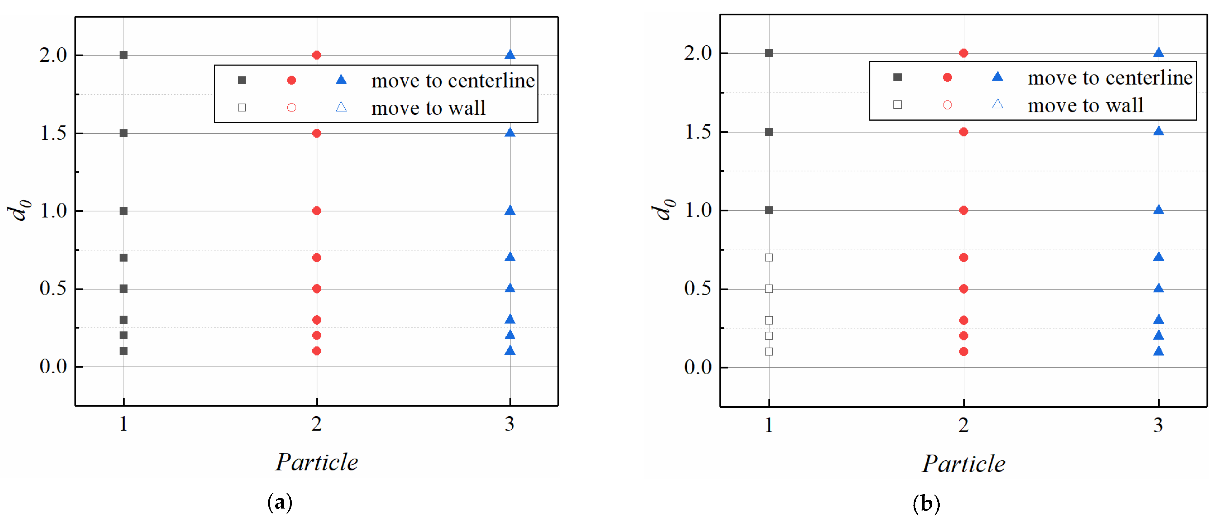
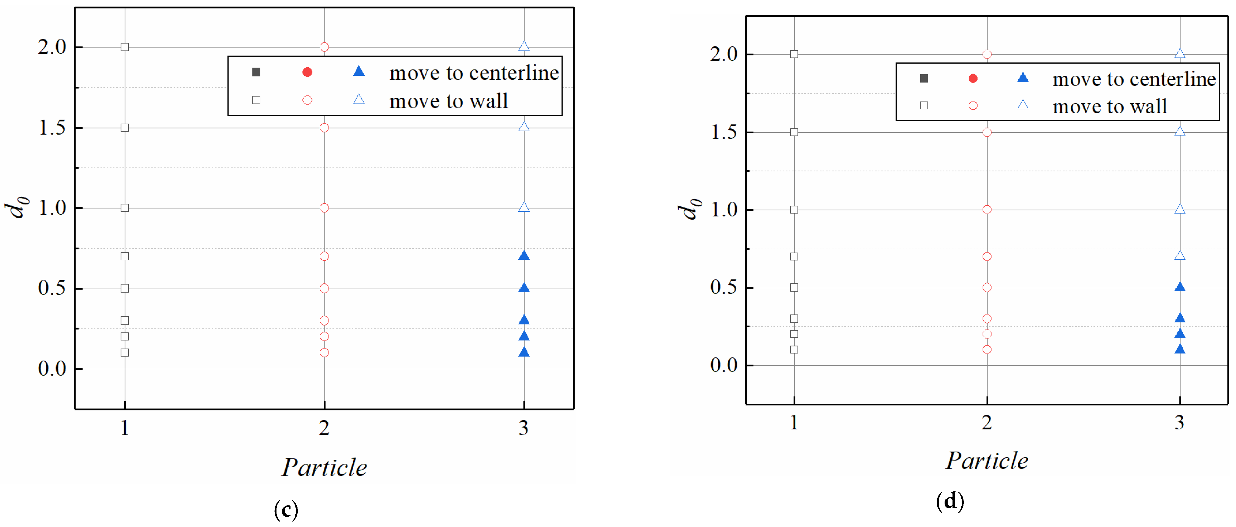
3.5. Abnormal Cross-Flow Migration of Particles

Based on the above results, a peculiar phenomenon has been found: in the Poiseuille flow of Giesekus fluid, which can make off-centerline single-particle migrate toward the centerline, one of the three particles would move abnormally because of the hydrodynamic interactions between the particles. Abnormal cross-flow migrations of particles induced by the hydrodynamic interaction between particles and other factors are investigated in this section. The viscoelasticity of the suspending fluid causes the particle cross-flow migration. The direction of particle migration is affected by the rheological properties, such as shear-thinning and the Weissenberg number. The shear-thinning effect causes particle migration toward the wall. The direction of particle migration for different particle initial positions (y₀) and different mobility parameters (α) is shown in Figure 14, where the direction of particle migration is dependent on the value of y₀ and α. It can be seen that we capture the separatrix (y_sep) (red dashed line) between the two directions. More particles move toward the centerline with the decrease in the shear-thinning effect and value of y₀.

Figure 15 shows the direction of three particles migration for different initial interparticle distances and different mobility parameters (α). Three particles migrate to the centerline when α = 0.1, as shown in Figure 15a, and the corresponding variation of interparticle distance is presented in Figure 7c. As shown in Figure 14, the particle with y₀ = 0.21 or less would migrate to the centerline at α = 0.3. However, particle 1 with y₀ = 0.2 would migrate to the wall at α = 0.3 when d_1,0 is less than or equal to 0.7, as shown in Figure 15b. On the contrary, the particle with y₀ = 0.19 or more would migrate to the wall at α = 0.5, as shown in Figure 14, while particle 3 with y₀ = 0.2 would migrate to the centerline at α = 0.5 when d_2,0 is less than or equal to 0.7, as shown in Figure 15c. The phenomenon similar wo Figure 15c also exists at α = 0.7, as shown in Figure 15d.

In order to explore the above phenomenon, we further study the trajectories of three particles with different initial interparticle distances and show the results in Figure 16. We can see that particle 1 first migrates to the wall for a distance Δm and then toward the centerline due to the interaction between particles. Here the distance Δm increases with decreasing in the initial interparticle distance d₀. The interparticle hydrodynamic interaction is the weakest for d₀ = 1.0, and so Δm is 0, as shown in Figure 16c. In Figure 16a, Δm is 0.0132 for d₀ = 0.8, i.e., the largest distance between particle 1 and the centerline is 0.2132. Nevertheless, the position of separatrix (y_sep) is 0.215. Between the separatrix and the centerline, particles would migrate toward the centerline, otherwise toward the wall. Consequently, particle 1 eventually moves to the centerline rather than to the wall. To summarize, if y₀ + Δm > y_sep, the particle changes direction and eventually migrates toward the wall. Otherwise, the particle keeps the original direction and moves to the centerline. In Figure 16, the differences in the trajectory between the single-particle and particle 1, single-particle and particle 3 are roughly marked Δn and Δk, respectively. It can be seen that the values of Δn and Δk are inversely proportional to the initial interparticle distance (d₀). Combining the results of Figure 15 and Figure 16, it can be inferred that the abnormal cross-flow migration of particles could be attributed to this interaction, and the hydrodynamic interaction is associated with the interparticle spacing, shear-thinning property and Weissenberg number. A detailed study would need to be carried out.

4. Conclusions

Migration and alignment of three interacting particles in Poiseuille flow of Giesekus fluids are investigated with the direct-forcing fictitious domain method. The model and method are validated by comparing the numerical results with the available data in the literature. The effects of the initial distance y₀ of particles from the centerline, the Weissenberg number (Wi), the shear-thinning effect and wall confinement on the migration and alignment of particles are analyzed. Conclusions are summarized as follows:

The main difference from the former work [23] is that the variation of off-centerline particle spacing is concentrated. The results reveal that the effect of y₀ on the migration and alignment of particles is significant. For y₀ = 0, particle 1 forms a pair with particle 2 when the initial interparticle distance d₀ is small, while there is no interaction among the three particles and the interparticle distances remain unchanged when d₀ is large. As the distance y₀ increases, the various type of particle spacing becomes more complex. When y₀ increases to 0.2, no particle pair is observed, and the interparticle distance becomes larger. For the off-centerline particle, the results show the evolution of particle spacing mainly occurs in the pathway of cross-flow migration, and the hydrodynamic interaction between particles becomes strong. The effect of the Weissenberg number is also studied. The increment of d₂ decreases with the increase in Wi in the case of the same increment of d₁. Additionally, as the shear-thinning effect becomes more pronounced, the maximum of d₁ increases and particle 1 forms a pair with particle 2 only when d_1,0 = d_2,0 = 0.1. The memory of shear-thinning is responsible for the reduction of d₁. The reduction of d₁ increases with the increase in α. For the effect of the confinement ratio, the bigger the confinement ratios, the stronger the polymer extension is.

What is more, particles would move abnormally in a three particles system. Three particles would migrate to the centerline for y₀ ≤ 0.2 when the shear-thinning effect is weak. As the shear-thinning effect increases, the particles tend to migrate toward the wall. When d₀ is small, the left particle first migrates to the wall for a distance and then toward the centerline, and the particle even changes the direction of migration completely, and this phenomenon is more obvious when d₀ is small. The abnormal migration of particles could be attributed to the interaction between particles, shear-thinning effect and Wi.

To extend this work, the formation of multi-particle trains and the abnormal migration would need to be investigated in detail. Furthermore, in order to better guide the practice, the internal mechanism needs to be investigated.

References

1. Pratt, E.D.; Huang, C.; Hawkins, B.G.; Gleghorn, J.P.; Kirby, B.J. Rare cell capture in microfluidic devices. Chem. Eng. Sci. 2011, 66, 1508–1522. [Google Scholar] [CrossRef] [Green Version]
2. Pedrol, E.; Massons, J.; Diaz, F.; Aguilo, M. Study of local inertial focusing conditions for spherical particles in asymmetric serpentines. Fluids 2020, 5, 1. [Google Scholar] [CrossRef] [Green Version]
3. Masaeli, M.; Sollier, E.; Amini, H.; Mao, W.; Camacho, K.; Doshi, N.; Mitragotri, S.; Alexeev, A.; Di Carlo, D. Continuous inertial focusing and separation of particles by shape. Phys. Rev. X 2012, 2, 031017. [Google Scholar] [CrossRef] [Green Version]
4. Ateya, D.A.; Erickson, J.S.; Howell, P.B., Jr.; Hilliard, L.R.; Golden, J.P.; Ligler, F.S. The good, the bad, and the tiny: A review of microflow cytometry. Anal. Bioanal. Chem. 2008, 391, 1485–1498. [Google Scholar] [CrossRef] [Green Version]
5. Godin, J.; Chen, C.; Cho, S.H.; Qiao, W.; Tsai, F.; Lo, Y. Microfluidics and photonics for bio-system-on-a-chip: A review of advancements in technology towards a microfluidic flow cytometry chip. J. Biophotonics 2008, 1, 355–376. [Google Scholar] [CrossRef] [PubMed] [Green Version]
6. Kersaudy-Kerhoas, M.; Dhariwal, R.; Desmulliez, M.P.Y. Recent advances in microparticle continuous separation. IET Nanobiotechnol. 2008, 2, 1–13. [Google Scholar] [CrossRef]
7. Kulrattanarak, T.; van der Sman, R.G.M.; Schroen, C.G.P.H.; Boom, R.M. Classification and evaluation of microfluidic devices for continuous suspension fractionation. Adv. Colloid Interface Sci. 2008, 142, 53–65. [Google Scholar] [CrossRef]
8. Kummrow, A.; Theisen, J.; Frankowski, M.; Tuchscheerer, A.; Yildirim, H.; Brattke, K.; Schmidt, M.; Neukammer, J. Microfluidic structures for flow cytometric analysis of hydrodynamically focussed blood cells fabricated by ultraprecision micromachining. Lab Chip 2009, 9, 972–981. [Google Scholar] [CrossRef]
9. Segré, G.; Silberberg, A. Radical particle displacements in Poiseuille flow of suspensions. Nature 1961, 189, 209–210. [Google Scholar] [CrossRef]
10. Karnis, A.; Mason, S.G. Particle motions in sheared suspensions. xix. viscoelastic media. Trans. Soc. Rheol. 1966, 10, 571–592. [Google Scholar] [CrossRef]
11. Villone, M.M.; D’Avino, G.; Hulsen, M.A.; Greco, F.; Maffettone, P.L. Numerical simulations of particle migration in a viscoelastic fluid subjected to Poiseuille flow. Comput. Fluids 2011, 42, 82–91. [Google Scholar] [CrossRef]
12. Villone, M.M.; D’Avino, G.; Hulsen, M.A.; Greco, F.; Maffettone, P.L. Particle motion in square channel flow of a viscoelastic liquid: Migration vs.secondary flows. J. Non-Newton. Fluid Mech. 2013, 195, 1–8. [Google Scholar] [CrossRef]
13. Spanjaards, M.M.A.; Jameson, N.O.; Hulsen, M.A.; Anderson, P.D. A Numerical Study of particle migration and sedimentation in viscoelastic Couette flow. Fluids 2019, 5, 25. [Google Scholar] [CrossRef] [Green Version]
14. Huang, P.Y.; Feng, J.; Hu, H.H.; Joseph, D.D. Direct simulation of the motion of solid particles in Couette and Poiseuille flows of viscoelastic fluids. J. Fluid Mech. 1997, 343, 73–94. [Google Scholar] [CrossRef] [Green Version]
15. Wang, P.; Yu, Z.; Lin, J.Z. Numerical simulations of particle migration in rectangular channel flow of Giesekus viscoelastic fluids. J. Non-Newton. Fluid Mech. 2018, 262, 142–148. [Google Scholar] [CrossRef]
16. Yu, Z.; Wang, P.; Lin, J.Z.; Hu, H. Equilibrium positions of the elasto-inertial particle migration in rectangular channel flow of Oldroyd-B viscoelastic fluids. J. Fluid Mech. 2019, 868, 316–340. [Google Scholar] [CrossRef]
17. Snijkers, F.; Pasquino, R.; Vermant, J. Hydrodynamic interactions between two equally sized spheres in viscoelastic fluids in shear flow. Langmuir 2013, 29, 5701–5713. [Google Scholar] [CrossRef]
18. Michele, J.; Patzold, R.; Donis, R. Alignment and aggregation effects in suspensions of spheres in non-Newtonian media. Rheol. Acta 1977, 16, 317–321. [Google Scholar] [CrossRef]
19. Choi, Y.J.; Hulsen, M.A. Alignment of particles in a confined shear flow of aviscoelastic fluid. J. Non-Newton. Fluid Mech. 2012, 175–176, 89–103. [Google Scholar] [CrossRef]
20. Xiang, N.; Dai, Q.; Ni, Z.H. Multi-train elasto-inertial particle focusing in straight microfluidic channels. Appl. Phys. Lett. 2016, 109, 134101. [Google Scholar] [CrossRef]
21. Pasquino, R.; Snijkers, F.; Grizzuti, N.; Vermant, J. The effect of particle size and migration on the formation of flow-induced structures in viscoelastic suspensions. Rheol. Acta 2010, 49, 993–1001. [Google Scholar] [CrossRef]
22. Pan, A.; Zhang, R.; Yuan, C.; Wu, H.Y. Direct measurement of microscale flow structures induced by inertial focusing of single particle and particle trains in a confined microchannel. Phys. Fluids 2018, 30, 102005. [Google Scholar] [CrossRef]
23. D’Avino, G.; Hulsen, M.A.; Maffettone, P.L. Dynamics of pairs and triplets of particles in a viscoelastic fluid flowing in a cylindrical channel. Comput. Fluids 2013, 86, 45–55. [Google Scholar] [CrossRef]
24. Glowinski, R.; Pan, T.-W.; Hesla, T.I.; Joseph, D.D. A distributed Lagrange multiplier/fictitious domain method for particulate flows. Int. J. Multiph. Flow 1999, 25, 755–794. [Google Scholar] [CrossRef]
25. Yu, Z.; Shao, X. A direct-forcing fictitious domain method for particulate flows. J. Comput. Phys. 2007, 227, 292–314. [Google Scholar] [CrossRef]
26. Yu, Z.; Wachs, A. A fictitious domain method for dynamic simulation of particle sedimentation in Bingham fluids. J. Non-Newton. Fluid Mech. 2007, 145, 78–91. [Google Scholar] [CrossRef]
27. Yu, Z.; Xia, Y.; Guo, Y.; Lin, J.Z. Modulation of turbulence intensity by heavy finite-size particles in upward channel flow. J. Fluid Mech. 2021, 913, 1140. [Google Scholar] [CrossRef]
28. Hu, H.H.; Patankar, N.A.; Zhu, M.Y. Direct numerical simulations of fluid-solid systems using the arbitrary Lagrangian–Eulerian technique. J. Comput. Phys. 2001, 169, 427–462. [Google Scholar] [CrossRef]
29. Joseph, D.D.; Liu, Y.J.; Poletto, M.; Feng, J. Aggregation and dispersion of spheres falling in viscoelastic liquids. J. Non-Newton. Fluid Mech. 1994, 54, 45–86. [Google Scholar] [CrossRef]
30. Daugan, S.; Talini, L.; Herzhaft, B.; Allain, C. Aggregation of particles settling in shear-thinning fluids. Part 1. Two-particle aggregation. Eur. Phys. J. E 2002, 7, 73–81. [Google Scholar] [CrossRef]
31. Yu, Z.; Wachs, A.; Peysson, Y. Numerical simulation of particle sedimentation in shear-thinning fluids with a fictitious domain method. J. Non-Newton. Fluid Mech. 2006, 136, 126–139. [Google Scholar] [CrossRef]
32. Dhahir, S.A.; Walters, K. On non-Newtonian flow past a cylinder in a confined flow. J. Rheol. 1989, 33, 781–804. [Google Scholar] [CrossRef]
33. Sullivan, M.T.; Moore, K.; Stone, H.A. Transverse instability of bubbles in viscoelastic channel flows. Phys. Rev. Lett. 2008, 101, 244503. [Google Scholar] [CrossRef] [Green Version]
Figure 1. Comparison of the lateral trajectory of a particle in a Poiseuille flow of Oldroyd-B fluid. (Wi = 0.5, Re = 0.5, ηr = 0.5, d/H = 0.15).
Fluids 06 00218 g001
Figure 2. Schematic diagram of three particles in a pressure-driven flow of viscoelastic fluid.
Fluids 06 00218 g002
Figure 3. Diverse variations of interparticle distances for different initial interparticle distances. (Wi = 0.5, α = 0.1, ηr = 0.3, ε = 0.3). (a) y0 = 0; (b) y0 = 0.1; (c) y0 = 0.15; (d) y0 = 0.2.
Fluids 06 00218 g003aFluids 06 00218 g003b
Figure 4. Variation of interparticle distances under more initial interparticle distances. (Wi = 0.5, α = 0.1, ηr = 0.3, ε = 0.3). (a) y0 = 0; (b) y0 = 0.2.
Fluids 06 00218 g004
Figure 5. The trajectories of three particles and the variation of interparticle spacing with time. (Wi = 0.5, α = 0.1, ηr = 0.3, ε = 0.3, y0 = 0.2). (a) d1,0 = d2,0 = 0.1; (b) d1,0 = d2,0 = 0.3. The thin red line represents t = 4: the stage of sharp change of particle spacing and cross-flow migration. The thin blue line represents t = 60: the stage of relatively stable particle spacing and particle migrate on the centerline.
Fluids 06 00218 g005
Figure 6. Pressure contours of different times for the three particles. (Wi = 0.5, α = 0.1, ηr = 0.3, ε = 0.3, y0 = 0.2). (a) t = 4; (b) t = 60.
Fluids 06 00218 g006
Figure 7. Diverse variations of interparticle distances for different initial interparticle distances and Wi. (α = 0.1, ηr = 0.3, ε = 0.3, y0 = 0.2). (a) Wi = 0.1; (b) Wi = 0.3; (c) Wi = 0.5; (d) Wi = 1.0; (e) Wi = 1.5.
Fluids 06 00218 g007
Figure 8. Polymer extension tr(B) along the pathway in Giesekus fluid at t = 7 (α = 0.1, ηr = 0.3, ε = 0.3, y0 = 0.2, d1,0 = d2,0 = 0.3). (a) Wi = 0.5; (b) Wi = 1.0; (c) Wi = 1.5.
Fluids 06 00218 g008
Figure 9. Diverse variations of interparticle distances for different initial interparticle distances and α (Wi = 0.5, ηr = 0.3, ε = 0.3, y0 = 0.1). (a) α = 0.1; (b) α = 0.3; (c) α = 0.5; (d) α = 0.7.
Fluids 06 00218 g009
Figure 10. Polymer extension tr(B) along the pathway in Giesekus fluid at t = 3 (Wi = 0.5, ηr = 0.3, ε = 0.3, y0 = 0.1, d1,0 = d2,0 = 0.3). (a) α = 0.1; (b) α = 0.3; (c) α = 0.5; (d) α = 0.7.
Fluids 06 00218 g010
Figure 11. Diverse variations of interparticle distances for different initial confinement ratios (Wi = 0.5, ηr = 0.3, α = 0.1, y0 = 0). (a) ε = 0.2; (b) ε = 0.3; (c) ε = 0.4.
Fluids 06 00218 g011aFluids 06 00218 g011b
Figure 12. Diverse variation of interparticle distances for different initial confinement ratios. (Wi = 0.5, ηr = 0.3, α = 0.1, y0 = 0.2). (a) ε = 0.2; (b) ε = 0.3; (c) ε = 0.4.
Fluids 06 00218 g012
Figure 13. Polymer extension tr(B) along the pathway in Giesekus fluid at t = 7 (Wi = 0.5, ηr = 0.3, α = 0.1, y0 = 0.1, d1,0 = d2,0 = 0.5). (a) ε = 0.2; (b) ε = 0.3; (c) ε = 0.4.
Fluids 06 00218 g013
Figure 14. Direction of particle migration for different particle initial positions and mobility parameters. (Wi = 0.5, ηr = 0.3, ε = 0.3).
Fluids 06 00218 g014
Figure 15. Direction of three particles migration for different initial interparticle distances and mobility parameters (Wi = 0.5, ηr = 0.3, ε = 0.3, y0 = 0.2) (a) α = 0.1; (b) α = 0.3; (c) α = 0.5; (d) α = 0.7.
Fluids 06 00218 g015aFluids 06 00218 g015b
Figure 16. Trajectories of particles for different initial interparticle distances (Wi = 0.5, ηr = 0.3, α = 0.3, ε = 0.3, y0 = 0.2) (a) d0 = 0.8; (b) d0 = 0.85; (c) d0 = 1.0.
Fluids 06 00218 g016aFluids 06 00218 g016b
Publisher’s Note: MDPI stays neutral with regard to jurisdictional claims in published maps and institutional affiliations.