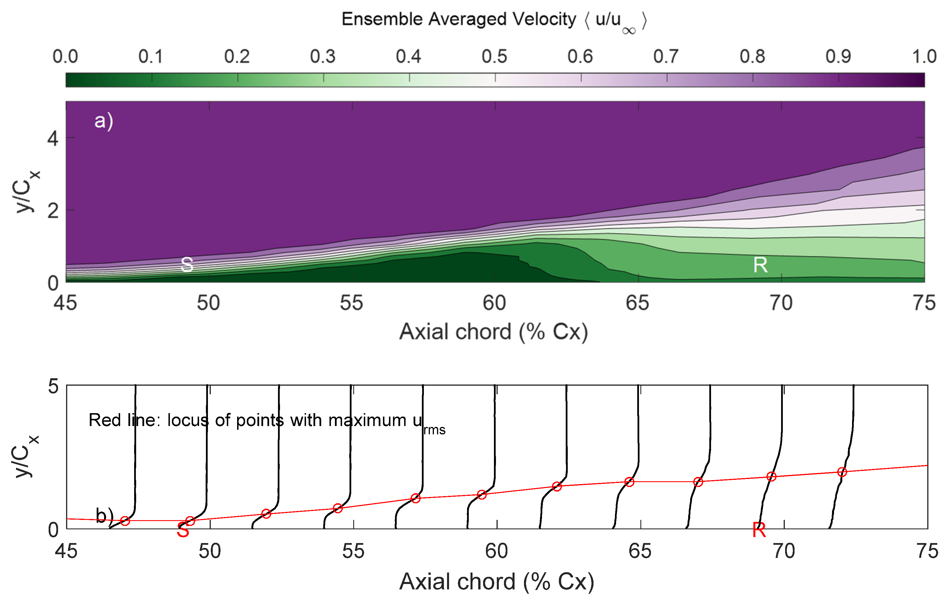
3.1. Time Domain Analysis
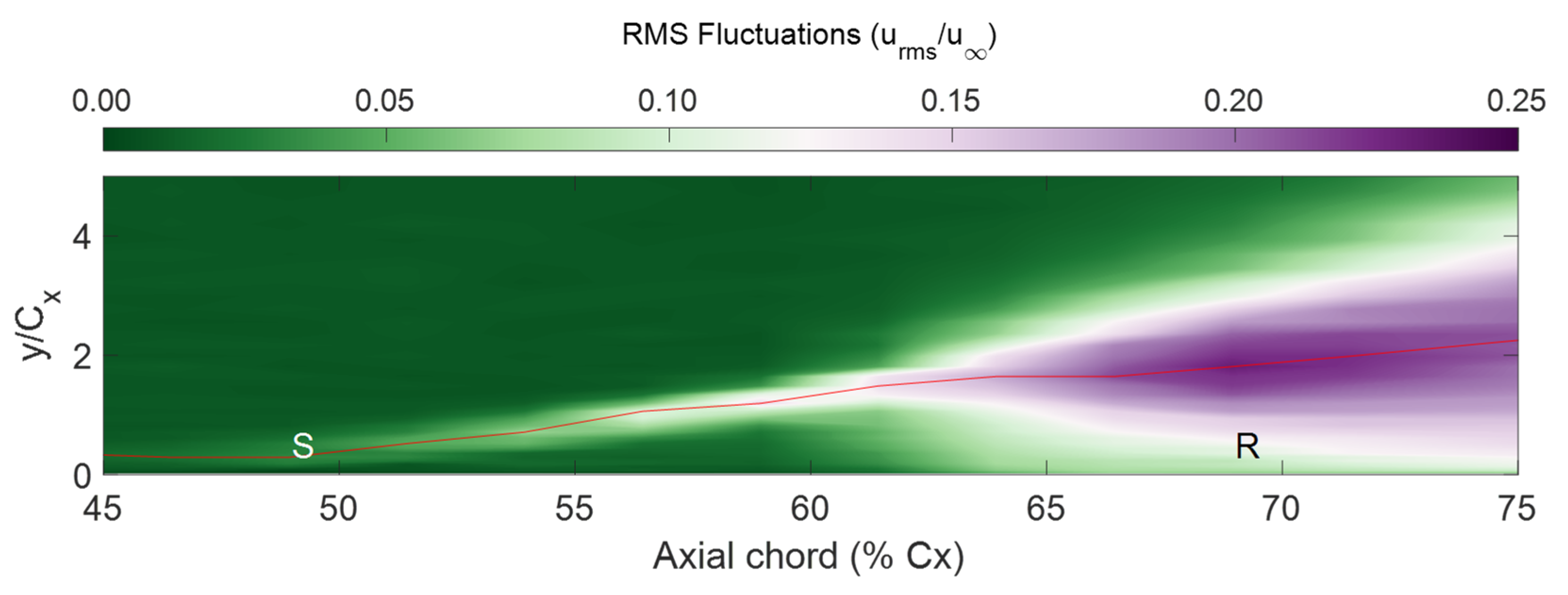
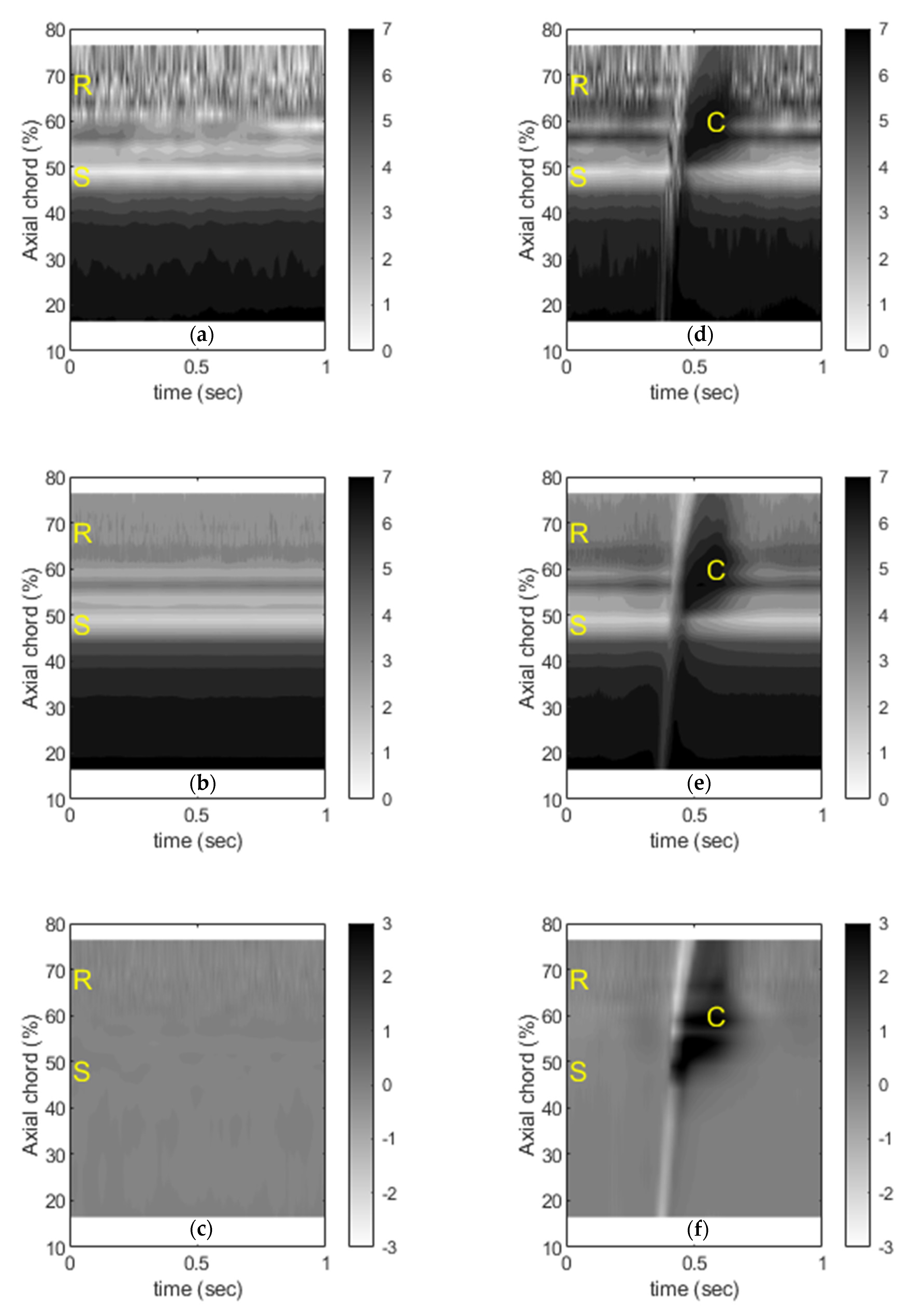
Figure 5 shows the space–time (S–T) diagram of the velocity signals acquired along the locus of the peak
. In each of the plots shown, the
-axis shows the time in seconds and the
-axis shows the streamwise location expressed as a percentage of the plate chord. The time axis shows one second’s worth of the signal and the space axis shows distances from 16% to 78% axial chord (0.16
to 0.78
) downstream of the plate leading edge. For comparison, the cases without (steady-inlet) and with the presence of the wake at the inlet to the test section (hereafter referred to as ‘wake-inlet’) are plotted side-by-side. The S–T diagrams of the raw velocity signals are presented first for the steady-inlet, in
Figure 5a, and for the wake-inlet, in
Figure 5d. In agreement with the
distribution over the surface, as shown earlier in
Figure 2, the velocity can be seen to decrease past the peak suction point (located near 0.4
) following the initial region of acceleration near the plate leading edge. The strong deceleration downstream of 0.4
causes the laminar boundary layer (seen with relatively smooth contours) to separate around 0.49
(the region annotated as S in the figure) and to reattach as a turbulent boundary layer (seen with streaky contours) around 0.69
(the region annotated as R in the figure). In reality, the streaky nature of the contours starts before reattachment at around 0.6
, which is slightly upstream of the peak height of the separation bubble. The instability of the shear layer is known to grow linearly over the front part of the separation bubble before becoming non-linear and triggering the formation of Kelvin–Helmholtz (K-H) vortex roll-up. This vortex roll-up enhances the process of flow breakdown into turbulence. In fact, the vortex structures ensure that high momentum fluid from the external flow is brought closer to the wall, thus enabling the separated flow to reattach back onto the surface. These observations are consistent with those of [
21,
22,
23]. The main difference between the steady-inlet case in
Figure 5a and the wake-inlet case in
Figure 5d is the presence of the convective disturbances due to the wake that is present for the latter. The wake is not only characterised by an ‘avenue’ of reduced velocity but also by a region of increased fluctuations, as seen by the ‘streakiness’ of the contours within the wake avenue in
Figure 5d. It is known [
12] that the wake as it impinges on the blade surface brings forward the location within the boundary layer where turbulence is present, although this turbulence is only partially present during the wake cycle in the upstream regions and only when the foot of the wake grazes the surface where the flow is laminar.
Another major difference between the steady-inlet case and the wake-inlet case is the appearance of a region of reduced fluctuations and increased velocity behind the wake deficit. This region is annotated as C in
Figure 5d–f and this corresponds to the ‘calmed region’. The calmed region is a relatively thin, non-stable passage of flow following a turbulent wake (or turbulent spot), resembling a ‘laminar region’. The perceived high velocities associated with region C are due to the passage of the calmed region momentarily making the boundary layer thinner and thus exposing the ‘freestream’ flow to the measurement probe. However, as noted in [
12], it would be erroneous to associate the properties of a laminar boundary layer with the calmed region. Although resistant to fluctuations, the skin friction under the calmed region is comparable to that in a turbulent flow, making it more resistant to adverse pressure gradients. The velocity variation within the calmed region is almost linear with the wall normal distance, resembling the laminar sublayer under a turbulent boundary layer but extending all the way to the freestream. This passage of ‘calmed’ flow relaxes back to that of a traditional laminar boundary layer after sufficient time.
Figure 5b,e essentially show the same data as in
Figure 5a,d but in the ensemble averaged form and thus the random fluctuations due to the disturbances are no longer visible. This clearly shows the separated region and its suppression partly during the time interval due to the arrival of the calmed region. In
Figure 5c,f, the evolution of the wake disturbance alone is isolated by subtracting the mean steady flow velocity field. This makes the contours of the velocity field due to the steady-inlet look uniform throughout, whereas that due to the wake-inlet shows the effect of the wake propagation alone.
More insight into the velocity field is available by plotting the individual velocity signals along the streamwise positions as shown in
Figure 6. For the steady-inlet case (
Figure 6a), the velocity field remains undisturbed and laminar until the separation point (~0.49
). The front portion of the bubble, often identified as the dead-air region [
24], is known to be a region of very low amplitude disturbances and linear evolution of disturbance is expected [
21]. As seen in
Figure 6a, the front part of the bubble (0.49
to 0.55
) is free from disturbances, although a low-frequency, low-amplitude, wavy structure seems to appear and grow towards the rear part of this region. However, by 0.59
, another relatively higher-frequency periodic structure is visible, which seems to grow rather rapidly before becoming unrecognisable due to the flow breakdown in the rear part of the bubble. A similar behaviour was observed by Diwan and Ramesh [
21], who identified that the growth of the disturbances could be broadly divided into to the mild-growth and small dispersion region before the separation point, a region of exponential growth from the front of the bubble to the peak height of the bubble and finally a region of nonlinear breakdown downstream of the peak bubble. The peak height of the bubble in the present measurement is located around 0.62
downstream of the plate leading edge.
For the wake-inlet case, as shown in
Figure 6b, the above observations from the stead-inlet case largely remain true. Two important differences are the additional features that exist within the wake disturbance itself (annotated by the letter W and enclosed within the green boxed region) and the calmed region that trails the wake disturbance (annotated by the letter C and demarcated by the purple boxed region). The convective wake disturbance is clearly identifiable in the upstream laminar boundary layer regions as a highly turbulent patch. One intriguing observation is that the diffusion (in the sense of temporal stretching of the signal) of the wake seems to be lower compared to that reported for a loudspeaker-generated wave packet in [
21]. This is despite similar levels of diffusion being present in the current study and that reported in [
21]. The calmed region was already visible, as described in
Figure 5, for the regions over the bubble; however, the time series of the signals indicate the presence of it even in the regions upstream of the bubble, which is less recognisable in the nominal laminar flow with a higher freestream velocity. As noted before, the calmed region is characterised by a thin boundary layer, its resistance to turbulent fluctuations and its ability to resist separation on the account of higher skin friction. The calmed region is seen to undergo dispersion (stretching) within the nominally laminar flow upstream and in the front portion of the boundary layer. However, as the disturbances grow towards the peak of the bubble and as the flow breaks down further downstream, the extent of the calming effect shrinks. There is also some evidence that some disturbances can penetrate into the calmed region downstream of the peak bubble height region. These disturbances seem to be of the periodic type, as noted earlier in the section, rather than the random fluctuation associated with turbulence. This aspect should become much clearer if one were to do a frequency domain analysis of the above signals. It may also help to elucidate the origins of the periodic structure that was noted upstream of the location of the peak bubble height.
3.2. Frequency Domain Analysis
The power spectra associated with the velocity signals seen in
Figure 6 are presented.
Figure 7 shows the spectra for both the steady-inlet and the wake-inlet cases with the same plot legend applicable to both. In general, the energy associated with the fluctuations increases as they grow with distance away from the leading edge. At any given streamwise location prior to the location of peak bubble height (0.62
), the wake-inlet signals have several orders of magnitude more energy than the steady-inlet signals. This is true across the entire frequency spectrum that is plotted and can be attributed to the energy of the fluctuations contained within the wake (higher turbulent content with moderate to high frequencies) and that associated with the velocity deficit within the wake (lower frequencies). The inertial subrange containing the Taylor micro-scale is usually associated with the −5/3rd power and is shown alongside the spectra in the plots (black solid line). It is apparent that the flow conforms to this regime post reattachment (0.62
) for the steady-inlet as well as the wake-inlet cases. A dominant feature of the spectra for both cases is the existence of a narrow frequency hump peaking at a frequency of 100 Hz (and its higher harmonics). It is notable that the energy contained in the hump becomes less dominant after reattachment, suggesting a break-up of flow producing turbulent structure in the inertial subrange. In other words, the inertial subrange only starts post-reattachment.
With several of the authors mentioned earlier [
9,
10,
11,
13,
14,
15] pointing to the possibility of the existence and dominance of amplified T–S waves and others (e.g., [
21]) observing the opposite, there is some interest in ascertaining the source of this frequency hump. Walker [
9] described a correlation for the most amplified T–S wave frequencies as a function of the displacement thickness-based Reynolds number (
), boundary layer edge velocity (
) and kinematic viscosity (
) of the form,
This was evaluated using the time-averaged velocity profiles for the steady-inlet case and the results are plotted in
Figure 8. The dominant frequency (
) is represented in Hz as well as in the circular frequency (
) form. The values for
immediately upstream and downstream of the separation bubble are approximately 45 Hz (circular frequency ~300 rad/s) and 5 Hz (circular frequency of ~30 rad/s), respectively. However, prior to the bubble,
decreases almost linearly from 160 Hz at a distance of 0.16
downstream of the plate leading edge until the front of the separation bubble.
Figure 8 tells us that a T–S wave with a frequency of 100 Hz could well be formed in the streamwise region close to 0.40
. These T–S disturbances could then become amplified in the free shear layer over the separation bubble as the latter is widely known to amplify upstream disturbances exponentially [
25]. The T–S waves and their frequencies, if present, may be predicted by linear stability theory and this requires obtaining the eigenvalues of the Orr–Sommerfeld equation. Such an analysis is currently not available for the present work. Since measurements using a single-wire CTA probe, as reported in this study, cannot resolve negative velocities that may be present within regions of the separation bubble with an inflectional profile, a
-based curve was fitted through the profiles (Dovgal et al. [
26]). This, however, only had a marginal effect on the T–S frequencies, as predicted by Equation (1).
Another phenomenon that could be the cause of the said frequency hump is the shear layer roll-up above the separation bubble that is known to occur due to the K–H instability. As noted by Simoni et al. [
27], the K–H instability is influenced by the adverse pressure gradient and flow velocity at separation (linked to the blade loading) and the vortex shedding frequency is influenced by the shear layer thickness. The above authors proposed an expression for the Strouhal number associated with the K–H instability as a function of the non-dimensional streamwise velocity (
), the streamwise velocity gradient (
) and the exit velocity-based Reynolds number (
) of the form,
where
is a constant. The authors of [
27] showed that for Reynolds numbers less than 300,000, the Strouhal number predicted by Equation (2) is within ±15% of the experimentally observed values for the test cases that they considered. For the present study, the Strouhal numbers evaluated in this manner corresponded to a frequency of 110 Hz near the peak height of the bubble and 95 Hz immediately downstream of the averaged bubble reattachment point. These numbers are extremely close to the experimentally observed frequency hump at 100 Hz and point to the dominance of K–H instability in this region.
The correlation-based analyses presented above and the proximity of the predicted frequencies to the experimentally observed frequency hump suggest a strong possibility of the existence of either phenomena. In other words, the origin of the frequency hump could be either the amplification of T–S waves (that originate in the close to 0.4
downstream of the plate leading edge) or the shear layer instability of the K–H type over the separation bubble. In the time series data presented in
Figure 6, periodic structures are visible at least as early as 0.59
.
Stieger and Hodson [
28] used a wavelet-based analysis of hot-film signals to reveal the presence of T–S waves when studying the wake-induced transition over a separated boundary layer on a flat plate. The above authors concluded that this highlighted the existence of natural transition phenomena between wake passing events. As in [
28], the current velocity signal data were also analysed using a Morlet wavelet (
) transform. The reason for selecting the Morlet wavelet is its resemblance to the wave packets found in the measured flow. Hughes and Walaker [
10] also used a Morlet wavelet for analysing their experimental data. As noted in [
10], the wavelet analysis helps with the identification of wave packets (with a specific frequency) that appear randomly in time under the influence of free-stream turbulence.
Figure 9 shows the contours of wavelet power corresponding to the location 0.59
downstream of the plate leading edge for both the steady-inlet and the wake-inlet cases. For the contours in each case, the corresponding velocity time series is shown above the contour map. Time is shown along the horizontal axis and frequency along the vertical logarithmic axis (base 2). The contour levels are also in the logarithmic scale (base 2). The black line is the 95% confidence enclosure. The advantage of the wavelet power spectrum as plotted in the above manner is that it combines both time and frequency information in one plot. It therefore makes it easier to understand the frequencies that are present at different instances within a given signal. For example,
Figure 9a allows us to identify, along its vertical axis, the most dominant frequency (100 Hz) corresponding to the frequency hump in the power spectrum that was presented earlier in
Figure 7. A horizontal red (dashed) line in
Figure 9a now signifies this dominant frequency. It is clear that, for the steady-inlet case, the velocity signal has a distinct 100 Hz spectral content at this location all along its length, with islands of highs (purple) and lows (green), pointing to the possibility that these could indeed be the amplified T–S waves that were potentially generated at a location close to 0.40
downstream of the plate leading edge. For the wake-inlet case, the wavelet power spectrum contours show a distinct region corresponding to the wake disturbance, which has fluctuations present within it in the full range of frequencies shown. Interestingly, the there are two distinct peaks visible within the wake corresponding to the frequency of 100 Hz. As in the steady-inlet case, fluctuations at 100 Hz are present all along the signal, except in the time gap of 0.5 s to 0.7 s, which can be identified as the calmed region. Therefore, if T–S wave amplification is indeed the cause of the 100 Hz spectral content at this location, then the wave is clearly damped within the calmed region.
Although not shown in the paper, for both steady- and wake-inlet cases, the wavelet power contours show that the amplitude of the 100 Hz fluctuations peaks close to the maximum bubble height location (0.62
), beyond which its distinctiveness is lost as the flow starts to break down non-linearly, thus bringing the higher-frequency regions highlighted in the contour plot. While the generation of T–S waves well upstream of the bubble and their amplification is a clear possibility, as suggested by the evaluation using Equation (2), the shedding frequency of the rolled-up vortices due to K–H instability is also in the 95–110 Hz region. In fact, a direct numerical simulation (DNS) study by McAuliffe and Yaras [
29] based on the results from a flat plate experimental test case has shown that both T–S and K–H instabilities can play a key role in the transition process if they occur at a similar frequency, as is the case in the present study. The above authors argued that although the K–H instability mechanism is key to the ultimate breakdown into turbulence, as it enables cross-stream mixing for the reattachment of the separated shear layer, the amplified T–S waves contribute considerably to the cross-stream momentum exchange in the separated shear layer. Furthermore, Diwan and Ramesh [
21] show evidence to modify the view that the origin of the inviscid instability in a bubble is related to the Kelvin–Helmholtz mechanism associated with the detached shear layer outside the bubble. They show that the inflectional instability associated with the separated shear layer is an extension of the instability of the upstream attached adverse pressure gradient boundary layer and the origin of the instability lies upstream of the separation bubble. They argue, further, that only when the separated shear layer has moved away sufficiently from the wall (e.g., peak height of the bubble) does the vorticity thickness-based non-dimensional frequency scale associated with K–H instability come into play and such a mode become dominant.


