Abstract
The momentum flux in a canonical turbulent boundary layer is known to have a time-series signature that is characterised by a highly intermittent variation, which includes very short periods of intense flux activity. Here, we study the variation in these flux signal characteristics across almost a decade of flow Reynolds number () by analysing datasets acquired using miniature cross-wire probes with matched spatial resolution. The analysis is facilitated by conditionally sampling the signal based on the quadrant (Qi; i = 1–4) and magnitude of the flux, revealing fractional cumulative contribution from Q4 to increase at a much faster rate than from Q2 with . An episodic description of the flux signal is subsequently undertaken, which associates this rapid increase in Q4 contributions with the emergence of extreme and rare flux events with . The same dataset is also used to test Townsend’s hypothesis on the active and inactive components of the momentum flux, which are obtained for the first time by implementing a spectral linear stochastic estimation-based decomposition methodology. While the active component is found to be the dominant contributor to the mean momentum flux consistent with Townsend’s hypothesis, the inactive component is found to be small but non-zero, owing to the non-linear interactions associated with the modulation phenomenon. Finally, an episodic description of the active and inactive momentum flux signal is undertaken to highlight the starkly different time series characteristics of the two flux components. The inactive flux signal is found to comprise individual statistically significant events associated with all four quadrants, leading to a small net contribution to the total flux.
1. Introduction and Motivation
The highly dissipative nature of zero-pressure gradient turbulent boundary layers (ZPG TBL) necessitates the continuous reinforcement of its turbulent kinetic energy (TKE) in order to maintain its quasi-steady-state characteristics [1,2]. This energy comes from the mean shear flow and is represented by the turbulence production term in the Reynolds transport equations. Analysis of the energy budget has been a topic of interest over many years [3,4,5,6], which has led to the association of these energy transfer mechanisms with coherent motions [6,7]. Reynolds shear stress (; where u and w denote the streamwise and wall-normal velocity fluctuations respectively and overbar denotes time average) also known as the mean momentum flux, forms a key component of the turbulence production term and has long been associated with the coherent motions, since the seminal flow visualisation studies of Kim et al. [8] and Corino and Brodkey [1]. Kim et al. [8], who experimentally tracked the near-wall flow using hydrogen bubbles, observed coherent motions associated with violent eruptions/bursting events (u < 0, w > 0) which, although short-lived, corresponded to high values of Reynolds shear stress. The significance of the coherent motions in turbulent energy production was reaffirmed by Corino and Brodkey [1], who in addition to bursting/ejections, also observed motions associated with the sweep events (u > 0, w < 0), also responsible for significant momentum flux.
The first quantitative evidence to prove the statistical significance of the ejections (∼70%) and sweep (∼50%) events, towards their contribution to , was presented through the pioneering cross-wire measurements of Wallace et al. [9] and Willmarth and Lu [10]. This was facilitated via the quadrant analysis proposed by Wallace et al. [9], which involved conditional sampling of the momentum flux signal as per the four possible quadrants (and the associated coherent motions) with respect to the sign of u and w: (i) Q1, outward interactions (u > 0, w > 0); (ii) Q2, ejections (u < 0, w > 0); (iii) Q3, inward interactions (u < 0, w < 0); and (iv) Q4, sweeps (u > 0, w < 0). Amongst these quadrants, contributions from Q1 and Q3 ( > 0) were estimated to be of much less significance and found to essentially offset the excess contributions from Q2 and Q4 by their opposite signs. To understand the nature of the flux signal, Willmarth and Lu [10] further sorted the time (t) series signal based on the magnitude of instantaneous momentum flux, following: > , where k is the threshold with possible values, k≥ 0. By systematically varying the value of k, they found that, while only 45% of the total signal had a magnitude greater than 0.5, these samples cumulatively accounted for nearly 99% of the mean momentum flux, revealing the intermittent character of its time series signal. Further, it was also found that all of the highly intense flux samples ( > 4) corresponded only to Q2 and Q4 and contributed approximately 60% of while being limited to only a small part (∼10%) of the time series. This analysis, hence, brought out the very unique variation in the magnitude of the momentum flux signal, which, as described in the words of Willmarth and Lu [10]: “is very small for a large fraction of time relative to shorter intervals of intense activity”. These temporal characteristics of the flux signal were noted at wall-normal locations across the shear layer [10,11], prompting the authors to associate the ejection phenomena with hairpin-shaped flow structures, exhibiting spatial coherence and comprising of intense vorticity [12]. Their hypothesis, which suggested spatial as well as temporal intermittency in the flux signal, was later confirmed with the advent of particle image velocimetry (PIV) technique [13,14]. These PIV-based studies, in fact, revealed association of the intense flux events with packets of hairpins (instead of individual hairpins), which explained the simultaneous multiple ejections noted by Bogard and Tiederman [15], Luchik and Tiederman [16] and Tardu [17] in the flux time-series.
The seminal work of Willmarth and co-workers [10,11,18] inspired the studies by Narasimha and co-workers [19,20], who attempted an episodic description of the flux signal acquired in the near-neutral atmospheric boundary layer (ABL). This involved representation of the flux time series as a combination of various statistically significant events contributing to , wherein an ‘event’ corresponded to a sequence of time series observations with a significant flux magnitude. Such a description was argued based on the fact that the other conventional methodologies of describing a time series, namely harmonic or wavelet descriptions, only explained contributions to the fluctuations of the time series (i.e., − ) instead of the mean () itself. In their analysis, the statistically significant flux events were detected based on a sorting criterion inspired from the one used previously by Willmarth and Lu [10]: > , where refers to the standard deviation of the flux signal and k is again the threshold. This criterion was found to be more robust, as compared to that used previously by Willmarth and co-workers [10,11]. In this manner, Narasimha et al. [20] were able to obtain a minimal description of the system by selecting an optimal k value, which led to the detection of the minimum number of events responsible for nearly all the mean flux. The low amplitude flux events which did not meet the optimal criterion (and hence contributed negligibly to ) were associated with passive or ‘inactive’ events as per the definition of Townsend [21,22], and were described as a background noise, comprising of signals with small and equal amplitude but opposite sign. Alternatively, those which did meet the criterion were considered as ‘active’ events [21,22] of the momentum flux and characterised as per the requirement of an episodic description. This involved defining the various event types, event amplitude, event duration, etc. for the active flux, which was found to be typical of a Poisson point process [23].
While a lot of effort has already been dedicated towards investigating the momentum flux signal over the past 50 years, most of the aforementioned studies [10,11,19,20] were conducted either at low in the laboratory ( ≲ 2000) or in the ABL, with each dataset having its own set of limitations. The data from the ABL are typically insufficient to achieve statistical convergence, as well as suffer from the varying stability conditions during the measurement. Studies conducted in the low regime, on the other hand, were predominantly focused in the near-wall/buffer region, owing to the peak in the turbulence production and TKE located in this region. Availability of high datasets in laboratory environments over time [24,25,26,27], however, has confirmed that contribution to the bulk production (at high ) comes from the logarithmic (log) region [28]. Further, the ability to simulate experimental conditions with high fidelity direct numerical simulation datasets [29,30,31] has revealed the possibility of significant measurement inaccuracies originating from poor spatial resolution while using cross-wire probes (or X-probes) in the near-wall region. These studies have inspired the development of miniature X-wire probes with sufficiently good resolution [26,27,29,31] for measuring velocity statistics in the high log-region. The availability of these high-fidelity datasets across a range of has also permitted application of several post-processing algorithms (e.g., spectral linear stochastic estimation (SLSE) [32,33]) to present empirical evidence [34,35] in support of Townsend’s attached eddy hypothesis (discussed briefly ahead in Section 1). The aforementioned experimental and theoretical developments, since the first measurements reported by Willmarth and co-workers [10,11], suggest the need to revisit the momentum flux analysis with sufficiently resolved high ZPG TBL datasets, which is attempted in the present study. Throughout this manuscript, u, v and w represent the velocity fluctuations along the streamwise (x), spanwise (y) and wall-normal (z) directions, respectively, while superscript ‘+’ denotes normalisation by the mean friction velocity () and kinematic viscosity (). Capital letters or overbars are used to indicate the time-averaged quantities, while lower case letters indicate fluctuations. The friction Reynolds number, = , with the boundary layer thickness. The words ‘structures’, ‘motions’ and ‘eddies’ used across the manuscript essentially conform to the definition of a coherent motion given by Robinson [7].
Townsend’s Attached Eddy Hypothesis
The attached eddy model of wall-turbulence (AEM [36,37]), which is based on Townsend’s attached eddy hypothesis [22], is one of the most popular and well cited conceptual models in the literature. As per this hypothesis, the kinematics in the log (or inertial) region of the canonical wall-bounded flow can be modelled by a hierarchy of inertially dominated (inviscid), geometrically self-similar attached eddies randomly distributed in the flow field. The term ‘attached’ here is used to refer to any coherent structure having a geometric extent scaling with its distance from the wall, z. These attached eddies, as per the hypothesis, have a population density inversely proportional to their height (), which can vary in the range () ≲ ≲ (), where refers to the beginning of the inertial region. The cumulative contribution from these eddies results in the logarithmic variation of the streamwise () and spanwise () variance in the inertial region ( < ≲ 0.15) while the wall-normal velocity variance () remains constant following:
where and are constants with ≈ −1. These expressions have received empirical support in recent literature [26,27,34,38,39,40], albeit with the recognition that other non-self-similar eddies play an important role at finite .
Noting the -dependence of and for a fixed in contrast to the -invariance of and depicted by Equation (1), Townsend [21] commented: “it is difficult to reconcile these observations without supposing that the motion at any point consists of two components, an active component responsible for turbulent transfer and determined by the stress distribution and an inactive component which does not transfer momentum or interact with the universal component”. As per his hypothesis, “the inactive motion is a meandering or swirling motion made up from attached eddies of large size which contribute to the Reynolds stress much further from the wall than the point of observation”. Thus, for a purely attached eddy-based flow (i.e., one in which the attached eddies are the only flow structures), the flow at any z in the inertial region is a combination of active and inactive contributions at z [21,22,35]. The active contributions come solely from the velocity fields of the attached eddies of height, ∼, which add to u(z), v(z), w(z) and consequently (z). The inactive contributions, on the other hand, come from the velocity fields of relatively tall and large attached eddies of height, ≪ < , which add to u(z) and v(z) but not to w(z) (and hence not to (z)). These differences are owing to the spatially localised nature of the w-velocity signature, in comparison to u- and v-signatures, from the attached eddies (illustrated in Figure 1 of Deshpande et al. [41]). Following the aforementioned discussion, the decomposition of the attached eddy fields may be expressed mathematically as per Panton [42]:
with subscript ‘a’ and ‘’ representing active and inactive contributions, respectively. According to the original hypothesis of Townsend [21,22], the inactive and active fields are uncorrelated [43], owing to which the Reynolds stresses listed in Equation (1) can be decomposed for a purely attached eddy field following:
Recently, Deshpande et al. [35,41] proposed an SLSE-based methodology to decompose the Reynolds stress components in Equation (3) and validated it by testing the active and inactive components for the various scaling arguments as per Townsend [21,22]. It was, however, found from their analysis that comprised of energy contributions from both self-similar as well as -scaled motions (i.e., superstructures [34,44]), wherein the latter, although not strictly conforming to the definition of an attached eddy [34,45,46], were argued to also have an inactive signature as per the definition of Townsend [21,22]. These superstructures, which span across the log-region, are known to modulate the relatively smaller (active) motions localised in the log-region and below via non-linear interactions [25,33,35,47,48,49]. Hence, contrary to Townsend’s hypothesis, the active and inactive motions cannot be deemed completely uncorrelated in a real TBL [50], resulting in the Reynolds stress decomposition in (3) to be redefined following [42]:
Considering Townsend’s hypothesis, however, the terms representing the non-linear interactions across the active and inactive motions would be expected to be much smaller than the respective Reynolds stress components (i.e., ≪ , ≪ , ≪ ). In the present study, we apply the active-inactive decomposition methodology proposed by Deshpande et al. [35] on existing high- X-probe datasets. The idea is to investigate the active () and inactive () momentum flux characteristics through the analysis strategies used by Willmarth and co-workers [10,11] and Narasimha and co-workers [19,20] and understand their relative statistical significance with respect to the mean total flux, .
2. ZPG TBL Datasets
The present study considers four published experimental ZPG TBL datasets [25,26], all of which have been acquired at the High Reynolds Number Boundary Layer Wind Tunnel (HRNBLWT) facility at the University of Melbourne. Table 1 lists these datasets along with necessary details associated with the individual experiments. The working section of the wind tunnel facility has a cross-section of ≃ 0.92 m × 1.89 m and operates under ZPG conditions as well as sufficiently low free-stream turbulence levels up to its maximum speed of 45 ms [24]. The unique feature of this facility is its very long working section length of 27 m, which permits generation of a high shear layer via growth of a physically thick turbulent boundary layer along the streamwise direction. Such an approach of investigating the TBL, popularly known as the ‘big and slow’ approach, allows one to conduct experiments over a range of without changing the free-stream speeds, thereby maintaining nominally the same smallest energetic scale (i.e., the viscous scale).

Table 1.
Summary of the various experimental ZPG TBL datasets analysed in the present study. Terminology associated with the geometry of the X-probe and other measurement parameters is described in Section 2.
Each dataset listed in Table 1 comprises measurements of the streamwise and wall-normal velocity components at 50 wall-normal locations across the TBL via the same miniature X-probe custom-built at Melbourne [29]. This probe comprised of two Wollaston wires each of diameter, d = 2.5 μm, spaced at a distance () 0.2 mm apart, with an etched sensor length of 0.5 mm (≈). Data were acquired at sufficiently high sampling rates and for a total time duration over several eddy turn over times (), to get well converged mean statistics. Amongst the four datasets mentioned in Table 1, those associated with the range 2500 ≲ ≲ 10,000 were acquired at the same free-stream speed of approximately 15 ms but with the X-probe placed at different streamwise (x) locations with respect to the start of the working section, leading to negligible variation in the viscous scale associated with the measurement. This permits investigation of the Reynolds number effects on the velocity statistics (demonstrated previously by Baidya et al. [26]) as well as on the momentum flux signal without any adverse influence of the spatial resolution effect [30,31].
The fourth dataset, however, is an exception in the sense that the high (≈15,000) was achieved by increasing the free-stream speed to ∼19 ms, leading to a slight drop in the viscous scale (and a corresponding increase in the viscous-scaled sensor geometry) as compared to the other three datasets. The unique aspect of this measurement, however, is its multi-point nature. The dataset comprises measurements of the skin-friction velocity fluctuations () synchronously with every X-probe measurement (u,w) across the TBL. These fluctuations were acquired using a hot-film sensor placed on the wall vertically below the X-probe sensor. Availability of this multi-point dataset permits application of the SLSE-based decomposition methodology proposed previously by Deshpande et al. [35] (Appendix A) to estimate the active and inactive components of the momentum flux (Equation (4)) for the present investigation.
3. Effect of Reτ
3.1. Conditional Sampling
The analysis begins by first investigating the effect of on the flux time series characteristics. This is facilitated by conditionally sampling the signal [51] acquired in the TBL across a range of (Table 1). The analysis is inspired from previous studies [9,10,20] discussed in Section 1 and is conducted using two sorting criteria:
- Criterion 1 is used to sort the flux samples in accordance to the particular quadrant (Q1–Q4) to which they belong using [9,10]:for i = 1, 2, 3 and 4. Thus, (t) demarcates the flux signal ((t)) into four segments ((t)) following:
- Criterion 2 is used to identify the fraction of the time series signal with flux magnitude beyond a pre-defined threshold, and it is given as per [10,20]:If suppose N samples of the time series (expressed as , with j = 1–N) are found to conform to the condition in (7) for a particular threshold k, then the fractional contribution to the mean flux from these N(k) samples may be defined asand the fractional cumulative time duration ((k)) for which the flux signal crosses the threshold is given by
By definition, (k = 0) = 1 and (k = 0) = 1. Criteria 1 and 2, defined above, may also be fused together to estimate the fractional contribution, to from the (k) samples in each of the four quadrants following [10]:
Here, and may be respectively related with and following:
Figure 1a shows the variation of and with respect to k for the momentum flux signals acquired at the nominal lower bound of the inertial region ( ≈ 100) at various . The respective curves for varying are found to overlap over one another, indicating invariance of the statistics with respect to the flow Reynolds number. A similar behaviour was noted when considering these curves at various in the inertial-region (not shown here), suggesting universality in these flux signal characteristics in the inertial region. The present analysis yields k ≈ 0.25 as the optimal, -invariant threshold [20], using which, one would recover nearly all (∼99%) of the mean flux from the minimum number of samples (∼58%). When the threshold is increased to k = 3, only ∼2% of the total samples have a magnitude greater than 3, but these samples are found to contribute approximately 30% of the mean flux. These results, which are analysed here in the inertial region, are consistent with the initial findings of Willmarth and Lu [10] in the near-wall region. Indeed, the flux signal has a very low magnitude for most of the time-signal, while the major contributions to the mean flux come from small intervals of intense activity. The present analysis provides empirical evidence to this interpretation over a decade of . It also establishes k = 0.25 as an optimal, -invariant threshold to extract the statistically significant part of the flux signal [20].
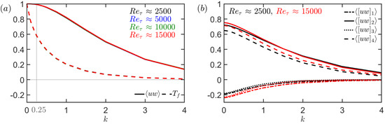
Figure 1.
(a) Fractional contribution to the mean flux, , and the cumulative fractional duration of the detected flux samples, , varying as a function of the threshold k used to detect these samples. (b) Fractional contribution to the mean flux demarcated into individual contributions from the four quadrants, (i = 1–4) varying as a function of k. All flux signals considered for this analysis were recorded at ≈ 100 at respective (indicated by various colours).
Figure 1b considers split into the individual contributions from the four quadrants, for i = 1–4, for the case of the highest and lowest . It is evident that ejections () contribute more to the mean flux than the sweeps (), irrespective of the variation in k, suggesting the former to be of relatively greater significance than the latter in the present range. This is consistent with observations made by Wallace et al. [9] and Willmarth and Lu [10]. Furthermore, contributions from Q1 and Q3 are found to be statistically less significant and simply nullify the excess contribution from Q2 and Q4, as noted by Willmarth and Lu [10]. Considering the effect of , contribution from all quadrants are found to increase with at k = 0. Interestingly, however, the contribution from Q4 increases at a much faster rate than Q2, suggesting that sweep events may become the dominant contributors to the mean flux at very high . This explains the observations made by Narasimha et al. [20] in the ABL at ∼ 10, who found percentage contribution from sweeps to be ∼79% of while ejections contributed ∼68%. On increasing k ≳ 1, the effect of on contributions from Q2 is found to be negligible. In case of Q4, on the other hand, an increment can be noted even for large k values, suggesting emergence of more intense sweep events with increase in . These observations motivate the need for a more detailed analysis of the instantaneous flux signal characteristics for varying , which is presented in the next subsection.
3.2. Episodic Description
We now attempt an episodic description of the momentum flux signal following Narasimha et al. [20], to better understand how the characteristics of the individual flux events in each quadrant are affected with varying . Here, we refer to an event as a sequence of time instants for which > , as depicted in Figure 2, with k = 0.25 being the optimal, -invariant threshold estimated in Section 3.1. To this end, we characterise the momentum flux events as per their various types, their amplitude and durations [20], each of which are schematically represented in Figure 2 and defined below:
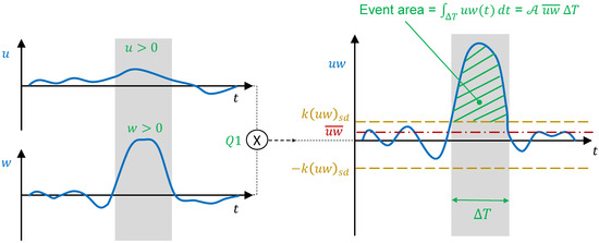
Figure 2.
Schematic depicting the characterisation of statistically significant flux event (highlighted with grey background) in accordance to the episodic description of the momentum flux signal proposed by Narasimha et al. [20]. Definition of the various terminologies is given in Section 3.2.
- Event type: For each event identified in the flux time series, the sign of the u and w samples at the corresponding instants is used to assign a particular quadrant (Q1–Q4) to which the event belongs.
- Event duration (): This refers to the time interval associated with the identified event and is expressed as .
- Event amplitude (): It is defined as , with essentially being the ratio of the average momentum flux over (obtained by computing the occupied area) to the mean momentum flux.
It should be noted here that is not sign definite and would vary depending on whether the event corresponds to Q2 and Q4 ( > 0) or Q1 and Q3 ( < 0).
Figure 3a–c shows the density scatter plots between the absolute value of the event amplitude () and its corresponding duration () for all the statistically significant events detected in the flux signals at ≈ 100, for various . The colour map represents the population density of the events, and hence differentiates the characteristics of the events that are more likely to happen (referred as common events) from the relatively ‘rare’ events. These event characteristics are further segregated in accordance to their respective quadrants, to bring out the similarities as well as differences between the events in the four quadrants. The density scatter plots reveal that the characteristics of these statistically significant events span over a range of time scales—from small , high events to large , small events—in all four quadrants. Such information, however, is obscured when representing the flux signal characteristics via statistics such as mean time duration [11], etc. At each , the maximum and values associated with the events in Q2 and Q4 are larger than those in Q1 and Q3, leading to a ‘bow-tie’ shaped asymmetric distribution of the event characteristics amongst the four quadrants. Q2 and Q4, quite understandably, also have a higher number of events associated with them than Q1 and Q3, which is reflected by the asymmetry in the colour map.
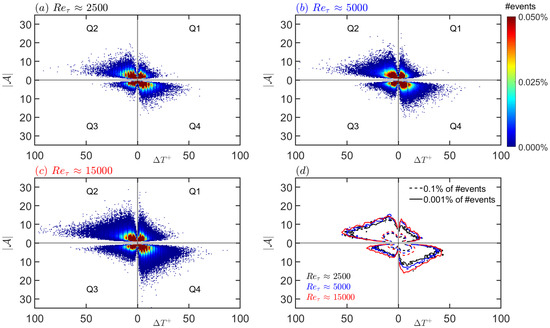
Figure 3.
(a–c) Density scatter plot between the absolute value of the flux event amplitude () and the associated viscous scaled duration () of the statistically significant events (using k = 0.25) at ≈ 100 for ≈: (a) 2500; (b) 5000; and (c) 15,000. The data are plotted in four quadrants to represent the characteristics of the events in the respective quadrants. The population density for a specific case is calculated by considering the statistically significant events from all four quadrants as a reference. (d) Constant density contours highlighting the changes in event characteristics for the relatively rare (0.001%) and common (0.1%) events as a function of (indicated by various colours).
Certain event characteristics, however, can be seen changing with increasing , such as the gradual spreading of the event amplitude and duration to greater magnitudes, which is better represented by the contour plot in Figure 3d. This plot considers how the contours of constant population density change with , where contours representing 0.001% density represent characteristics of relatively rare events in comparison to the more common events (0.1% density). In general, the rare events are observed to spread out towards larger and with increase in . However, this spread is more significant for events corresponding to Q4 as compared to the other quadrants, in particular the high and small events in Q4. It is the emergence of these rare and extreme events, which can be considered responsible for the increased contribution from to the mean flux (Figure 1b) at very high [20]. Interestingly, though, these increments tend to be balanced out in the mean by respective increments in Q1 and Q3 keeping ≈ −1 in the log-region at all [25,26]. The present analysis, thus, encourages further investigation into the emergence of extreme events in the TBL with increasing . Such events are responsible for the non-Gaussian tails in the probability distribution function of the flux signal, and hence are of significance to the meteorological community interested in predicting ABL turbulence [20,52].
4. Active and Inactive Momentum Flux
4.1. Estimating the Active and Inactive Flux Signal
With the characteristics for the total flux signal () now established, we investigate its sub-components, i.e., the active () and inactive () parts of the momentum flux (Equation (4)), which can be obtained here only for the multi-point dataset of Talluru et al. [25]. To this end, we implement the SLSE-based decomposition methodology (Appendix A) proposed by Deshpande et al. [35] to obtain at a wall-normal location () corresponding to the inertial region following:
where = (()) is the Fourier transform of the skin-friction velocity fluctuation, in time. Further, corresponds to a complex-valued, scale-specific transfer kernel between the synchronously acquired u(z) and , and it is defined as per [33]:
where the asterisk (∗) and curly brackets () denote the complex conjugate and ensemble averaging, respectively. Interested readers may refer to Appendix A for the complete procedure followed to arrive at Equation (12). It is worth noting that the SLSE-based energy decomposition is carried out here only as a function of the frequency domain, owing to the limitations of the dataset, as opposed to that for both the frequency and spanwise wavenumber in case of Deshpande et al. [35]. Following (12), the time domain equivalent of can be estimated simply by the inverse Fourier transform:
with known, the time series of the active component () at can be obtained following (2):
Figure 4a,b depicts a portion of the u-time series and its corresponding active and inactive sub-components at ≈ 100 as an example. is found to resemble the small-scale (high frequency) characteristics of u, given its association with motions localised at (active). , on the other hand, represents large-scale variations owing to its association with taller/inactive motions, and has a very low magnitude for most of the time.
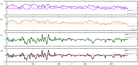
Figure 4.
(a,b) Example of a u-time series at ≈ 100 (in (a)) decomposed into its active and inactive components (in (b)). The w-time series synchronously acquired at the same is also plotted in (b). (c,d) Comparison of the total flux time series () computed from u- and w-time series in (a), with its corresponding (c) active and (d) inactive component.
The availability of the time series of both active and inactive streamwise components, along with the synchronously measured w (Figure 5a), permits the estimation of the respective momentum flux time series following Equation (4). The active and inactive components of the momentum flux are respectively compared with the total flux () in Figure 4c,d. can be seen to follow the -signal reasonably well, suggesting the active part of the momentum flux to be the dominant contributor to , consistent with the hypothesis of Townsend [21,22]. In contrast, the magnitude of -signal is close to zero for the majority of the signal, except in certain instants where both , w≠ 0.
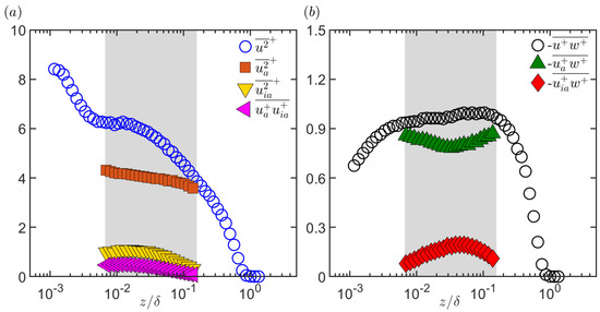
Figure 5.
Viscous scaled (a) streamwise turbulence intensity and (b) momentum flux profiles from the dataset of Talluru et al. [25], decomposed into their respective active and inactive components following (4) for in the inertial region (indicated by the grey shaded region).
To analyse the statistical significance of the active and inactive components across the inertial region, Figure 5b shows all the mean momentum flux components (active, inactive and total) estimated by using Equations (12)–(15) for various . The individual components obtained via decomposition of the streamwise turbulence intensity (; Equation (4)) are also plotted for comparison in Figure 5a. It is evident that the active part () represents the dominant contribution to the mean momentum flux [21,22]. However, it is also worth noting the non-zero contribution from (≈ 0.15), which may be ascertained to the non-linear interactions (such as the modulation phenomenon) between the superstructure signatures in and the predominantly active signatures in w [21,22,35,50]. A similar interaction can also be noted between the active and inactive components of the streamwise velocity (), which is estimated to be of the same order (≈0.3) as . The order of magnitude similarity between these two components is consistent with the comparable values of the amplitude modulation coefficient, estimated by Talluru et al. [25], for both u and w components. It should be noted here that the statistical trends depicted in Figure 5, such as , ≠ 0, conflict with the original hypothesis of Townsend [21,22], which was based on the assumption of a TBL comprising solely active and inactive motions (both of which are associated with the attached eddies). The differences can be ascertained to the coexistence of non-self-similar motions such as superstructures, fine dissipative scales, etc. in a real TBL [35], which also contribute to each sub-component of the Reynolds stresses (apart from the attached eddies).
Next, the investigation is directed towards analysing the time-series characteristics of the and signals, as done previously for the -signal in Section 3. Readers interested in the analysis of the normal Reynolds stress components (, , ) are referred to the work by Deshpande et al. [35,41] for a detailed discussion on that topic.
4.2. Conditional Sampling
We begin the analysis of the and signals by first estimating the fractional contribution from the statistically significant active and inactive flux samples to the mean momentum flux, . For this, we extend the same sorting criteria (Criteria 1 and 2) defined previously in Equation (10) (Section 3.1) to and following:
with and , respectively, referring to the number of detected samples in the active and inactive flux signals for the quadrant i and threshold k. It should be noted that both and are computed here with respect to the mean momentum flux () to estimate the fractional contribution to the total flux. Following (11), the cumulative fractional contributions as well as the total number of statistically significant samples for and can be calculated using (16) and (17) following:
Similarly, the fractional cumulative duration for which the two signals lie beyond a pre-defined threshold can be expressed as:
Figure 6a shows the variation of , , and , , with respect to k from the respective momentum flux signals at ≈ 100 at ≈ 15,000. The nature of variation of the active contributions (), for varying threshold values, is similar to the full flux signal (), with the vertical offset nominally equivalent to . A similar nature of variation was also noted when the respective flux signals were analysed at different in the inertial region (not shown here). Extending the concept of obtaining a minimal description of the flux signal [20] to active and inactive components, k = 0.25 is found as an effective threshold to recover ∼99% of as well as by considering the minimum number of samples – ≈ 0.5 and ≈ 0.25. While ≈ 0.25 is comprehensible given the very dormant state of the signal seen in Figure 4d, the fact that ≈ 0.5 indicates that even the active flux signal comprises of statistically insignificant events (with respect to the mean flux), which is in contrast to the hypothesis of Narasimha et al. [20]. Interestingly, ≈ 0 for k≳ 1.5, suggesting that nearly all inactive contributions could be removed from the total flux signal by setting the threshold at k = 1.5. This criterion, however, cannot be used to segregate the active and inactive components of the -signal since it also removes significant contributions (∼40%) from the active flux signal. It is important to note that ≈ 0 does not indicate ≈ 0, motivating the investigation into the latter in Figure 6b.
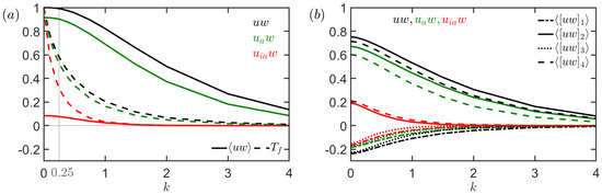
Figure 6.
(a) Fractional contribution to mean total flux, and the cumulative fractional duration of the detected flux samples, varying as a function of the threshold k used to detect these samples. (b) Fractional contribution to flux demarcated into individual contributions from the four quadrants, (i = 1–4) varying as a function of k. Black, green and red lines respectively represent these statistics for the total (), active () and inactive () flux signals computed at ≈ 100 for ≈ 15,000.
On sorting the -signal based on the individual contributions from the four quadrants, the nature of variation of is seen to be similar to . Contributions from Q2 and Q4 are found to be significantly more than those from Q1 and Q3 for all k. On the other hand, behaves starkly different to these two. Contributions from all four quadrants are nearly equal irrespective of the variation of k, indicating the positive (Q1 and Q3) and negative (Q2 and Q4) flux events tend to nearly cancel out each other, subsequently resulting in ≪ . It is important to note here that, while (k = 0) ≈ 0.1, ≈ ≈ 0.2 at k = 0, which is a non-negligible fraction of the mean flux. This suggests the presence of individual statistically significant events in the -signal, motivating a detailed characterisation of these events, as done above in Section 3.2.
4.3. Episodic Description
We now extend the episodic description of the flux signal [20] to the and -signal by following the same definitions of the event type, amplitude and duration as given above in Section 3.2, with for all signals normalised by . Figure 7a–c shows the density scatter plots between the absolute value of the event amplitude () and its corresponding duration () for all the statistically significant events (k = 0.25) detected in , and -signal at ≈ 100. As would be expected based on the observations in Figure 4 and Figure 6, distribution of the event characteristics for the -signal are found to be similar to those seen in the -signal. The density scatter plots, in particular, bring out the clear differences between the characteristics of the active and inactive flux events in the four quadrants. The key difference is that the ‘bow-tie’ shaped asymmetric distribution of the event characteristics, noted for both or , is not observed for . This is because the maximum of the inactive flux events, associated with Q2 and Q4, is significantly smaller than that for the or flux events. Interestingly, the characteristics of the inactive flux events are distributed in a quasi-symmetric manner about = 0 axis, suggesting events in Q1 and Q2 being of nearly equal intensity (but of opposite sign) than those in Q4 and Q3, respectively. This symmetry is also noted for the population density of the inactive events, which is more clearly reflected by the constant density contours in Figure 7d, explaining why ≪ . It is worth noting here that, although most of the ‘rare’, yet extreme events (∼0.001% density), which have high and short , are present in the -signal, the -signal does not correspond solely to weak amplitude events, with the maximum ≈ 10. Hence, although inactive events do not contribute substantially to the mean, the present analysis suggests that these motions should not be disconsidered while modelling turbulent flows given their statistical relevance in the instantaneous sense.
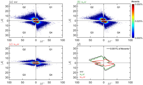
Figure 7.
(a–c) Density scatter plot between the absolute value of the flux event amplitude () and the associated viscous scaled duration () of the statistically significant events (using k = 0.25) in the (a) , (b) and (c) signals at ≈ 100 for ≈ 15,000. The data are plotted in four quadrants to represent the characteristics of the events in the respective quadrants. The population density is calculated by considering the statistically significant events found in the respective signals from all four quadrants as a reference. (d) Constant density contours highlighting the changes in event characteristics for the various flux signals (indicated by different colours).
5. Conclusions
The present paper revisits the momentum flux analysis, conducted almost half a century ago by Willmarth and co-workers [10,11] and Wallace et al. [9], with sufficiently resolved ZPG TBL datasets now available, varying over a range of [25,26]. Inspired from the aforementioned studies, the flux signals acquired in the log-region are conditionally sampled based on: (i) the (u,w) quadrant to which the samples belong; and (ii) the magnitude of the momentum flux. The analysis on the new datasets yields results consistent with the initial findings of Willmarth and Lu [10], revealing the highly intermittent nature of the momentum flux signal. While contributions from the second quadrant (Q2; ejections) are found to be more significant than from the fourth (Q4; sweeps) for the present datasets, the comparison over almost a decade change of suggests the relative contributions from the latter to be increasing at a much faster rate than the former with . Notably, these increased contributions from Q4 (with ) are found to be associated with highly intense flux events, which are balanced by much milder increments in Q1 and Q3 contributions to yield ≈ −1 at all . This unique behaviour of the Q4 contributions is further characterised via the episodic description methodology by Narasimha et al. [20], which reveals the high amplitude and short duration (i.e., extreme) nature of these events. More importantly, these extreme events are estimated to be a rare occurrence, suggesting the inherent difficulty in prediction of such statistically significant events for very high ABL phenomenon.
Analysis along the same lines is also later extended to the active and inactive components [21,22] of the momentum flux, which are obtained by implementing the SLSE-based methodology proposed recently by Deshpande et al. [35]. The active component of the flux is found to be the dominant contributor to the mean momentum flux () across the inertial region, providing the first empirical evidence to the hypothesis of Townsend [21,22]. Accordingly, the signal characteristics of this flux component are very similar to that exhibited by the total flux. On the other hand, the inactive flux component, which was hypothesised by Townsend [21,22] to be nominally zero for a purely attached eddy field, is found to make non-zero contributions to . These contributions are likely associated with the non-linear interactions, in the form of modulation [25,33,48], between the superstructures and the active motions in the inertial region of a ZPG TBL. Conditional sampling of the inactive flux signal revealed almost equal but non-negligible (≈0.2) fractional contribution from all four quadrants, suggesting individual inactive flux events to be of statistical significance, despite ≪ . This was reaffirmed by undertaking the episodic description of the inactive flux signal, which revealed the presence of short duration events with sufficiently high amplitude (≈10) from Q1 and Q4, suggesting inactive events should be considered while attempting turbulence modelling of instantaneous flow phenomena.
Author Contributions
Conceptualisation, R.D. and I.M.; methodology, R.D.; software, R.D.; validation, R.D.; formal analysis, R.D.; investigation, R.D.; resources, I.M.; writing—original draft preparation, R.D.; writing—review and editing, R.D. and I.M.; supervision, I.M.; project administration, I.M.; and funding acquisition, I.M. All authors have read and agreed to the published version of the manuscript.
Funding
This research was funded by the Australian Research Council.
Institutional Review Board Statement
Not applicable.
Informed Consent Statement
Not applicable.
Data Availability Statement
Data available on request from the authors.
Acknowledgments
We are grateful to Talluru et al. [25] and Baidya et al. [26] for making their respective data available. This work was motivated by the seminal work of W. W. Willmarth and co-workers, and we are very pleased to be able to contribute to these proceedings celebrating his distinguished career.
Conflicts of Interest
The authors declare no conflict of interest. The funders had no role in the design of the study; in the collection, analyses, or interpretation of data; in the writing of the manuscript, or in the decision to publish the results.
Abbreviations
The following abbreviations are used in this manuscript:
| ABL | atmospheric boundary layer |
| HRNBLWT | high Reynolds number boundary layer wind tunnel |
| PIV | particle image velocimetry |
| SLSE | spectral linear stochastic estimation |
| TBL | turbulent boundary layer |
| TKE | turbulent kinetic energy |
| ZPG | zero pressure gradient |
Appendix A. SLSE-Based Methodology to Decompose the Flux Time Series
This section demonstrates the methodology to estimate a component of the u-time series at any wall-normal location (say ), representing contributions from certain specific coherent motions coexisting at , via the spectral linear stochastic estimation (SLSE) approach. The procedure outlined here has been merely adapted from earlier studies introducing SLSE [32,33], which can be directly referred for a detailed understanding on this technique. According to this approach, a scale-specific conditional output at is obtained from a scale-specific unconditional input at following:
where is the Fourier transform of in time, t. Here, represents the scale-specific linear transfer kernel and the superscript E represents the estimated quantity. Such an approach enables an estimation of those scales at which are also coherent with . For this, is computed from an ensemble of data following:
with and the scale-specific phase and gain, respectively, and the asterisk (∗), curly brackets () and vertical bars () denoting the complex conjugate, ensemble averaging and modulus, respectively. For the case of ≪ , would be representative of the energy contributions from all coexisting motions significantly taller than , which as per the discussion in Deshpande et al. [35] leads to:
where represents the inactive component of the streamwise velocity.
References
- Corino, E.R.; Brodkey, R.S. A visual investigation of the wall region in turbulent flow. J. Fluid Mech. 1969, 37, 1–30. [Google Scholar] [CrossRef]
- Tennekes, H.; Lumley, J.L. A First Course in Turbulence; MIT Press: Cambridge, MA, USA, 1972. [Google Scholar]
- Lumley, J.L. Spectral energy budget in wall turbulence. Phys. Fluids 1964, 7, 190–196. [Google Scholar] [CrossRef]
- Domaradzki, J.A.; Liu, W.; Härtel, C.; Kleiser, L. Energy transfer in numerically simulated wall-bounded turbulent flows. Phys. Fluids 1994, 6, 1583–1599. [Google Scholar] [CrossRef]
- Mizuno, Y. Spectra of energy transport in turbulent channel flows for moderate Reynolds numbers. J. Fluid Mech. 2016, 805, 171. [Google Scholar] [CrossRef]
- Lee, M.; Moser, R.D. Spectral analysis of the budget equation in turbulent channel flows at high Reynolds number. J. Fluid Mech. 2019, 860, 886–938. [Google Scholar] [CrossRef]
- Robinson, S.K. Coherent motions in the turbulent boundary layer. Annu. Rev. Fluid Mech. 1991, 23, 601–639. [Google Scholar] [CrossRef]
- Kim, H.; Kline, S.J.; Reynolds, W. The production of turbulence near a smooth wall in a turbulent boundary layer. J. Fluid Mech. 1971, 50, 133–160. [Google Scholar] [CrossRef]
- Wallace, J.M.; Eckelmann, H.; Brodkey, R.S. The wall region in turbulent shear flow. J. Fluid Mech. 1972, 54, 39–48. [Google Scholar] [CrossRef]
- Willmarth, W.W.; Lu, S.S. Structure of the Reynolds stress near the wall. J. Fluid Mech. 1972, 55, 65–92. [Google Scholar] [CrossRef]
- Lu, S.S.; Willmarth, W.W. Measurements of the structure of the Reynolds stress in a turbulent boundary layer. J. Fluid Mech. 1973, 60, 481–511. [Google Scholar] [CrossRef]
- Willmarth, W.W.; Tu, B.J. Structure of turbulence in the boundary layer near the wall. Phys. Fluids 1967, 10, S134–S137. [Google Scholar] [CrossRef]
- Adrian, R.J.; Meinhart, C.D.; Tomkins, C.D. Vortex organization in the outer region of the turbulent boundary layer. J. Fluid Mech. 2000, 422, 1–54. [Google Scholar] [CrossRef]
- Ganapathisubramani, B.; Longmire, E.K.; Marusic, I. Characteristics of vortex packets in turbulent boundary layers. J. Fluid Mech. 2003, 478, 35–46. [Google Scholar] [CrossRef]
- Bogard, D.G.; Tiederman, W.G. Burst detection with single-point velocity measurements. J. Fluid Mech. 1986, 162, 389–413. [Google Scholar] [CrossRef]
- Luchik, T.S.; Tiederman, W.G. Timescale and structure of ejections and bursts in turbulent channel flows. J. Fluid Mech. 1987, 174, 529–552. [Google Scholar] [CrossRef]
- Tardu, S. Characteristics of single and clusters of bursting events in the inner layer. Exp. Fluids 1995, 20, 112–124. [Google Scholar]
- Wei, T.; Willmarth, W.W. Reynolds-number effects on the structure of a turbulent channel flow. J. Fluid Mech. 1989, 204, 57–95. [Google Scholar] [CrossRef]
- Narasimha, R.; Kailas, S.V. Turbulent bursts in the atmosphere. Atmos. Environ. Part A Gen. Top. 1990, 24, 1635–1645. [Google Scholar] [CrossRef]
- Narasimha, R.; Kumar, S.R.; Prabhu, A.; Kailas, S.V. Turbulent flux events in a nearly neutral atmospheric boundary layer. Philos. Trans. R. Soc. Math. Phys. Eng. Sci. 2007, 365, 841–858. [Google Scholar] [CrossRef]
- Townsend, A.A. Equilibrium layers and wall turbulence. J. Fluid Mech. 1961, 11, 97–120. [Google Scholar] [CrossRef]
- Townsend, A. The Structure of Turbulent Shear Flow, 2nd ed.; Cambridge University Press, Ed.; Cambridge University Press: Cambridge, UK, 1976. [Google Scholar]
- Cox, D.R.; Isham, V. Point Processes; CRC Press: Boca Raton, FL, USA, 1980; Volume 12. [Google Scholar]
- Marusic, I.; Chauhan, K.; Kulandaivelu, V.; Hutchins, N. Evolution of zero-pressure-gradient boundary layers from different tripping conditions. J. Fluid Mech. 2015, 783, 379–411. [Google Scholar] [CrossRef]
- Talluru, K.M.; Baidya, R.; Hutchins, N.; Marusic, I. Amplitude modulation of all three velocity components in turbulent boundary layers. J. Fluid Mech. 2014, 746. [Google Scholar] [CrossRef]
- Baidya, R.; Philip, J.; Hutchins, N.; Monty, J.P.; Marusic, I. Distance-from-the-wall scaling of turbulent motions in wall-bounded flows. Phys. Fluids 2017, 29, 020712. [Google Scholar] [CrossRef]
- Baidya, R.; Philip, J.; Hutchins, N.; Monty, J.P.; Marusic, I. Spanwise velocity statistics in high-Reynolds-number turbulent boundary layers. J. Fluid Mech. 2021, 913. [Google Scholar] [CrossRef]
- Marusic, I.; Mathis, R.; Hutchins, N. High Reynolds number effects in wall turbulence. Int. J. Heat Fluid Flow 2010, 31, 418–428. [Google Scholar] [CrossRef]
- Baidya, R. Multi-Component Velocity Measurements in Turbulent Boundary Layers. Ph.D. Thesis, Department of Mechanical and Manufacturing Engineering, University of Melbourne, Parkville, Australia, 2016. [Google Scholar]
- Baidya, R.; Philip, J.; Hutchins, N.; Monty, J.P.; Marusic, I. Spatial averaging effects on the streamwise and wall-normal velocity measurements in a wall-bounded turbulence using a cross-wire probe. Meas. Sci. Technol. 2019, 30, 085303. [Google Scholar] [CrossRef]
- Deshpande, R.; Monty, J.P.; Marusic, I. A scheme to correct the influence of calibration misalignment for cross-wire probes in turbulent shear flows. Exp. Fluids 2020, 61, 1–17. [Google Scholar] [CrossRef]
- Tinney, C.; Coiffet, F.; Delville, J.; Hall, A.; Jordan, P.; Glauser, M. On spectral linear stochastic estimation. Exp. Fluids 2006, 41, 763–775. [Google Scholar] [CrossRef]
- Baars, W.J.; Hutchins, N.; Marusic, I. Spectral stochastic estimation of high-Reynolds-number wall-bounded turbulence for a refined inner-outer interaction model. Phys. Rev. Fluids 2016, 1, 054406. [Google Scholar] [CrossRef]
- Baars, W.J.; Marusic, I. Data-driven decomposition of the streamwise turbulence kinetic energy in boundary layers. Part 2. Integrated energy and A1. J. Fluid Mech. 2020, 882, A26. [Google Scholar] [CrossRef]
- Deshpande, R.; Monty, J.P.; Marusic, I. Active and inactive components of the streamwise velocity in wall-bounded turbulence. J. Fluid Mech. 2021, 914, A5. [Google Scholar] [CrossRef]
- Perry, A.; Chong, M. On the mechanism of wall turbulence. J. Fluid Mech. 1982, 119, 173–217. [Google Scholar] [CrossRef]
- Marusic, I.; Monty, J.P. Attached eddy model of wall turbulence. Annu. Rev. Fluid Mech. 2019, 51, 49–74. [Google Scholar] [CrossRef]
- Jimenez, J.; Hoyas, S. Turbulent fluctuations above the buffer layer of wall-bounded flows. J. Fluid Mech. 2008, 611, 215–236. [Google Scholar] [CrossRef]
- Lee, M.; Moser, R.D. Direct numerical simulation of turbulent channel flow up to Reτ ≈ 5200. J. Fluid Mech. 2015, 774, 395–415. [Google Scholar] [CrossRef]
- Orlandi, P.; Bernardini, M.; Pirozzoli, S. Poiseuille and Couette flows in the transitional and fully turbulent regime. J. Fluid Mech. 2015, 770, 424–441. [Google Scholar] [CrossRef]
- Deshpande, R.; Monty, J.P.; Marusic, I. Active and inactive motions in wall turbulence. In Proceedings of the 22nd Australasian Fluid Mechanics Conference, Brisbane, Australia, 7–10 December 2020. [Google Scholar]
- Panton, R.L. Composite asymptotic expansions and scaling wall turbulence. Philos. Trans. R. Soc. A Math. Phys. Eng. Sci. 2007, 365, 733–754. [Google Scholar] [CrossRef]
- Bradshaw, P. ‘Inactive’ motion and pressure fluctuations in turbulent boundary layers. J. Fluid Mech. 1967, 30, 241–258. [Google Scholar] [CrossRef]
- Hutchins, N.; Marusic, I. Evidence of very long meandering features in the logarithmic region of turbulent boundary layers. J. Fluid Mech. 2007, 579, 1–28. [Google Scholar] [CrossRef]
- Yoon, M.; Hwang, J.; Yang, J.; Sung, H.J. Wall-attached structures of streamwise velocity fluctuations in an adverse-pressure-gradient turbulent boundary layer. J. Fluid Mech. 2020, 885, A12. [Google Scholar] [CrossRef]
- Deshpande, R.; Chandran, D.; Monty, J.; Marusic, I. Two-dimensional cross-spectrum of the streamwise velocity in turbulent boundary layers. J. Fluid Mech. 2020, 890, R2. [Google Scholar] [CrossRef]
- Morrison, J.F. The interaction between inner and outer regions of turbulent wall-bounded flow. Philos. Trans. R. Soc. A Math. Phys. Eng. Sci. 2007, 365, 683–698. [Google Scholar] [CrossRef] [PubMed]
- Mathis, R.; Hutchins, N.; Marusic, I. Large-scale amplitude modulation of the small-scale structures in turbulent boundary layers. J. Fluid Mech. 2009, 628, 311–337. [Google Scholar] [CrossRef]
- Wu, S.; Christensen, K.; Pantano, C. Modelling smooth- and transitionally rough-wall turbulent channel flow by leveraging inner–outer interactions and principal component analysis. J. Fluid Mech. 2019, 863, 407–453. [Google Scholar] [CrossRef]
- McNaughton, K.G.; Brunet, Y. Townsend’s hypothesis, coherent structures and Monin–Obukhov similarity. Bound.-Layer Meteorol. 2002, 102, 161–175. [Google Scholar] [CrossRef]
- Kovasznay, L.S.G.; Kibens, V.; Blackwelder, R.F. Large-scale motion in the intermittent region of a turbulent boundary layer. J. Fluid Mech. 1970, 41, 283–325. [Google Scholar] [CrossRef]
- Sapsis, T.P. Statistics of extreme events in fluid flows and waves. Annu. Rev. Fluid Mech. 2021, 53. [Google Scholar] [CrossRef]


Publisher’s Note: MDPI stays neutral with regard to jurisdictional claims in published maps and institutional affiliations. |
© 2021 by the authors. Licensee MDPI, Basel, Switzerland. This article is an open access article distributed under the terms and conditions of the Creative Commons Attribution (CC BY) license (https://creativecommons.org/licenses/by/4.0/).