
A Model of Synovial Fluid with a Hyaluronic Acid Source: A Numerical Challenge


Abstract
1. Introduction
2. Model
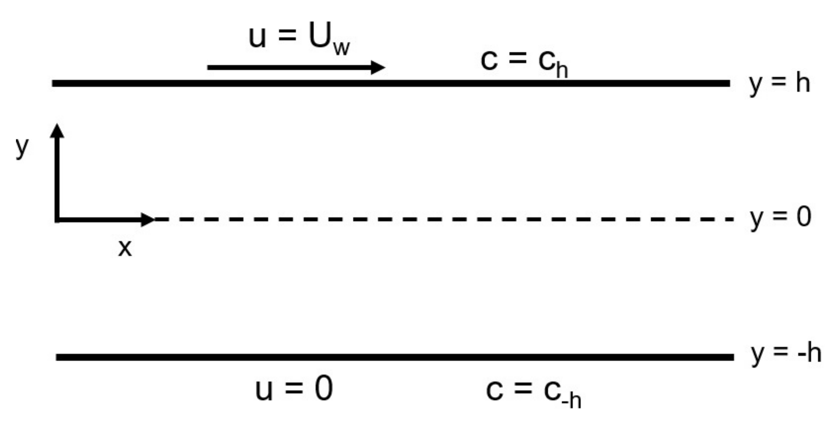
2.1. Equations
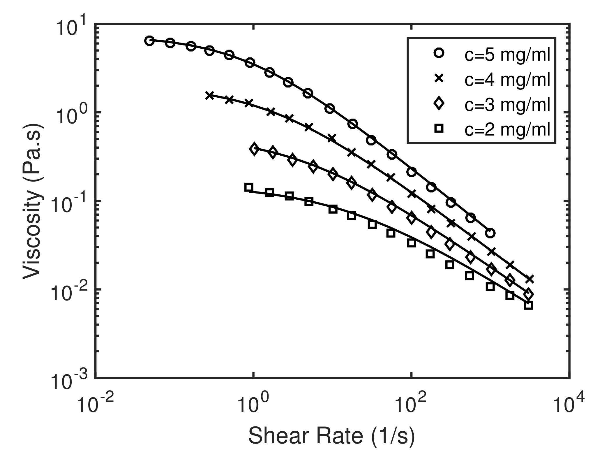
2.2. Viscosity Model
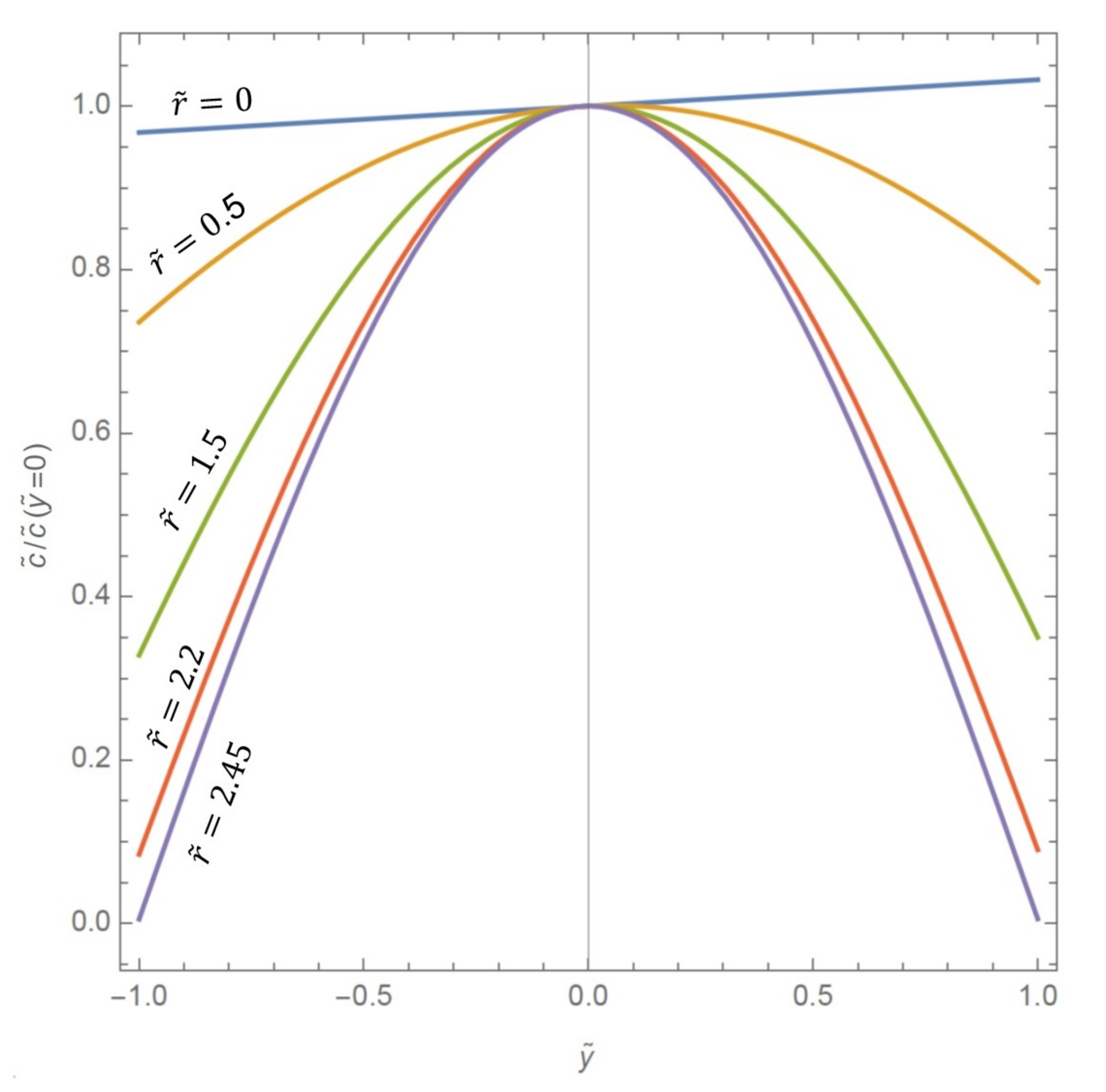
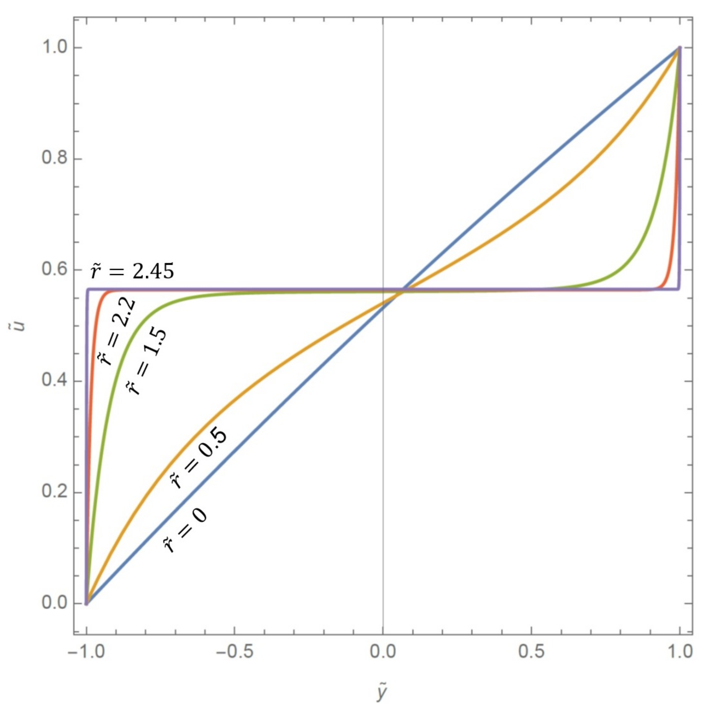
2.3. Analysis of the Model: Steady State
2.4. Stability Consideration
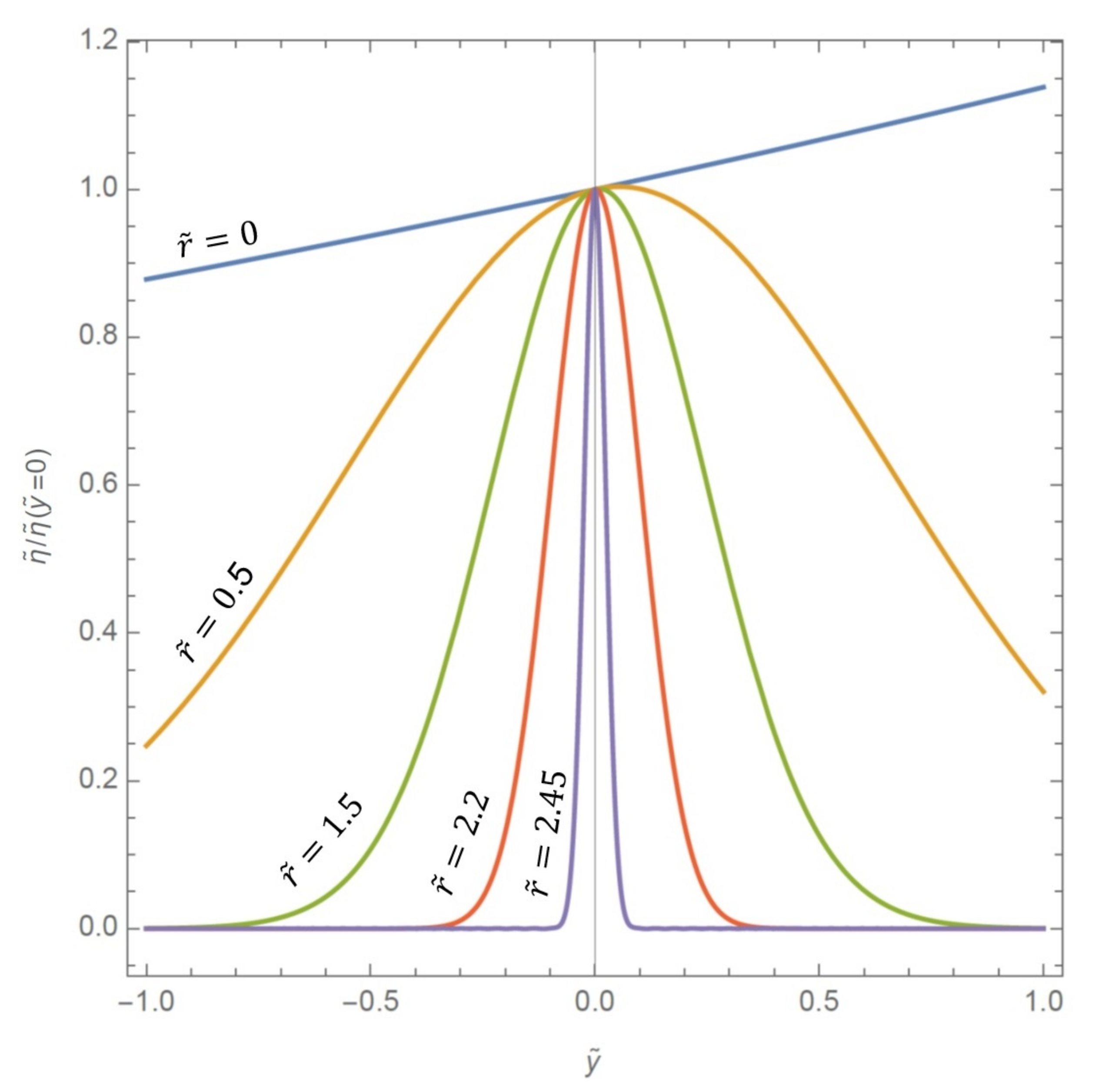
3. Results
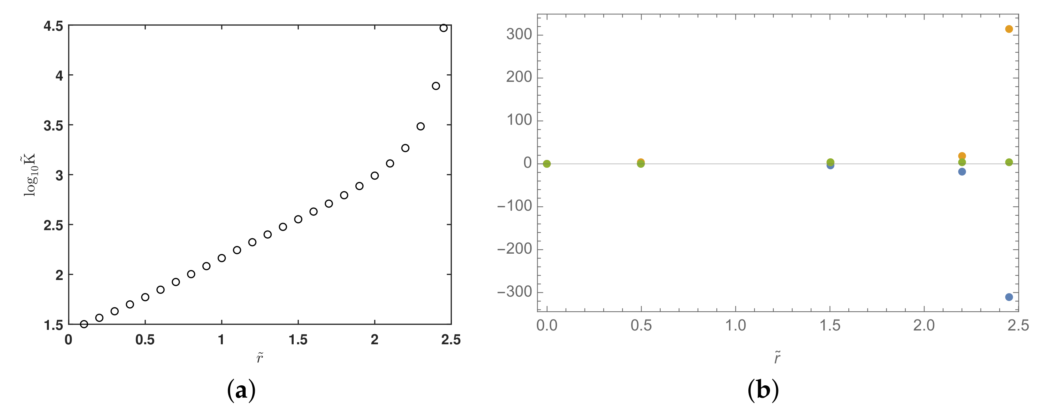
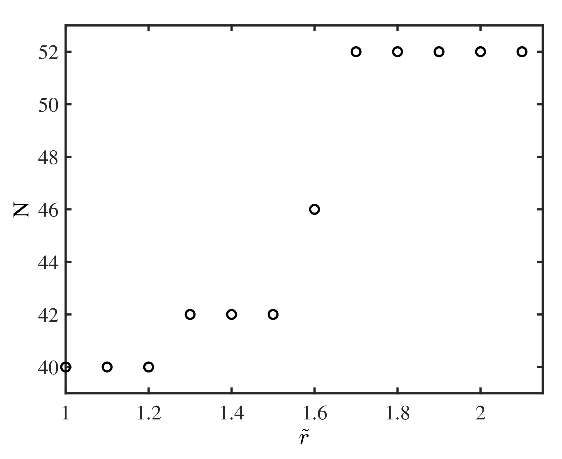
4. Discussion about Numerics
5. Conclusions
Author Contributions
Funding
Institutional Review Board Statement
Informed Consent Statement
Data Availability Statement
Acknowledgments
Conflicts of Interest
Nomenclature
| c | concentration | |
| dimensionless concentration | - | |
| D | diffusion coefficient | |
| h | half distance between the plates | m |
| K | stress | |
| dimensionless stress | - | |
| n | flow behavior index | - |
| r | strength of the source term | 1/s |
| dimensionless strength of the source term | - | |
| t | time | s |
| dimensionless time | - | |
| u | velocity | m/s |
| dimensionless velocity | - | |
| wall velocity | m/s | |
| viscosity | kg/m/s | |
| zero-shear viscosity | kg/m/s | |
| dimensionless viscosity | - | |
| Cross time constant | s | |
| density |
Abbreviations
| SF | Synovial fluid |
| HA | Hyaluronic acid |
| CSC | Chebyshev spectral collocation |
| Re | Reynolds number |
| Pe | Péclet number |
Appendix A. Numerical Treatment of the Problem
Appendix A.1. Spatial Discretization
Appendix A.2. Temporal Discretization
References
- Fam, H.; Bryant, J.; Kontopoulou, M. Rheological Properties of Synovial Fluids. Biorheology 2007, 44, 59–74. [Google Scholar] [PubMed]
- Ogston, A.; Stanier, J. On the State of Hyaluronic Acid in Synovial Fluid. Biochem. J. 1950, 46, 364. [Google Scholar] [CrossRef] [PubMed]
- Ogston, A.; Stanier, J. The Physiological Function of Hyaluronic Acid in Synovial Fluid; Viscous, Elastic and Lubricant Properties. J. Physiol. 1953, 119, 244. [Google Scholar] [CrossRef] [PubMed]
- King, R. A rheological measurement of three synovial fluids. Rheol. Acta 1966, 5, 41–44. [Google Scholar] [CrossRef]
- Ruggiero, A.; Sicilia, A. Lubrication modeling and wear calculation in artificial hip joint during the gait. Tribol. Int. 2020, 142, 105993. [Google Scholar] [CrossRef]
- Hron, J.; Málek, J.; Pustějovská, P.; Rajagopal, K. On the Modeling of the Synovial Fluid. Adv. Tribol. 2010, 2010, 104957. [Google Scholar] [CrossRef]
- Fam, H.; Kontopoulou, M.; Bryant, J. Effect of Concentration and Molecular Weight on the Rheology of Hyaluronic Acid/Bovine Calf Serum Solutions. Biorheology 2009, 46, 31–43. [Google Scholar] [CrossRef]
- Seller, P.; Dowson, D.; Wright, V. The Rheology of Synovial Fluid. Rheol. Acta 1971, 10, 2–7. [Google Scholar] [CrossRef]
- Conrad, B.P. The Effects of Glucosamine and Chondroitin on the Viscosity of Synovial Fluid in Patients with Osteoarthritis. Ph.D. Thesis, University of Florida, Gainesville, FL, USA, 2001. [Google Scholar]
- Tandon, P.; Bong, N.; Kushwaha, K. A New Model for Synovial Joint Lubrication. Int. J. Bio Med. Comput. 1994, 35, 125–140. [Google Scholar] [CrossRef]
- Rudraiah, N.; Kasiviswanathan, S.; Kaloni, P. Generalized Dispersion in a Synovial Fluid of Human Joints. Biorheology 1990, 28, 207–219. [Google Scholar] [CrossRef]
- Mazzucco, D.; McKinley, G.; Scott, R.D.; Spector, M. Rheology of Joint Fluid in Total Knee Arthroplasty Patients. J. Orthop. Res. 2002, 20, 1157–1163. [Google Scholar] [CrossRef]
- Ruggiero, A. Milestones in Natural Lubrication of Synovial Joints. Front. Mech. Eng. 2020, 6, 52. [Google Scholar] [CrossRef]
- Hor, C.H.; Tso, C.P.; Chen, G.M.; Chee, K.K. Characteristics of the Internal Fluid Flow Field Induced by an Oscillating Plate with the other Parallel Plate Stationary. J. Adv. Res. Fluid Mech. Therm. Sci. 2019, 55, 136–141. [Google Scholar]
- Pekkan, K.; Nalim, R.; Yokota, H. Computed Synovial Fluid Flow in a Simple Knee Joint Model. In Fluids Engineering Division Summer Meeting, Honolulu, Hawaii, USA; Proceedings of the ASME: New York, NY, USA, 2003; Volume 1, pp. 2085–2091. [Google Scholar] [CrossRef]
- Afsar Khan, A.; Farooq, A.; Vafai, K. Impact of induced magnetic field on synovial fluid with peristaltic flow in an asymmetric channel. J. Magn. Magn. Mater. 2018, 446, 54–67. [Google Scholar] [CrossRef]
- Romanishina, T.A.; Romanishina, S.A.; Deeva, V.S.; Slobodyan, S.M. Numerical modeling of synovial fluid layer. In Proceedings of the 2017 IEEE International Young Scientists Forum on Applied Physics and Engineering (YSF), Lviv, Ukraine, 17–20 October 2017; pp. 143–146. [Google Scholar] [CrossRef]
- VijayaKumar, R.; Ratchagar, N.P. Mathematical Modeling of Synovial Joints with Chemical Reaction. J. Phys. Conf. Ser. 2021, 1724, 012051. [Google Scholar] [CrossRef]
- Bridges, C.; Rajagopal, K. Pulsatile Flow of a Chemically-Reacting Nonlinear Fluid. Comput. Math. Appl. 2006, 52, 1131–1144. [Google Scholar] [CrossRef]
- Bridges, C.; Karra, S.; Rajagopal, K. On Modeling the Response of the Synovial Fluid: Unsteady Flow of a Shear-Thinning, Chemically-Reacting Fluid Mixture. Comput. Math. Appl. 2010, 60, 2333–2349. [Google Scholar] [CrossRef]
- Uguz, A.K.; Massoudi, M. Heat Transfer and Couette Flow of a Chemically Reacting Non-Linear Fluid. Math. Methods Appl. Sci. 2010, 33, 1331–1341. [Google Scholar] [CrossRef]
- Massoudi, M.; Uguz, A. Chemically-Reacting Fluids with Variable Transport Properties. Appl. Math. Comput. 2012, 219, 1761–1775. [Google Scholar] [CrossRef]
- Trefethen, L.N. Spectral Methods in MATLAB; Society for Industrial and Applied Mathematics (SIAM): Oxford, England, 2000; Volume 10. [Google Scholar]
- Labrosse, G. Méthodes Spectrales; Ellipses: Paris, France, 2011. [Google Scholar]
- Guo, W.; Labrosse, G.; Narayanan, R. The Application of the Chebyshev-Spectral Method in Transport Phenomena: Lecture Notes in Applied and Computational Mechanics; Springer-Verlag: Berlin/Heidelberg, Germany, 2013; Volume 68. [Google Scholar]
- Cohen, A.M. Numerical Methods for Laplace Transform Inversion; Springer: Boston, MA, USA, 2007; Volume 5. [Google Scholar]
- Ma, D.; Saunders, M. Solving Multiscale Linear Programs Using the Simplex Method in Quadruple Precision. In Numerical Analysis and Optimization; Al-Baali, M., Grandinetti, L., Purnama, A., Eds.; Springer Springer International Publishing: Cham, Switzerland, 2015; Volume 134, pp. 223–235. [Google Scholar]
- Carson, E.; Higham, N. A New Analysis of Iterative Refinement and Its Application to Accurate Solution of Ill-Conditioned Sparse Linear Systems. SIAM J. Sci. Comput. 2017, 39, A2834–A2856. [Google Scholar] [CrossRef]
- Yang, L.; Yurkovich, J.; Lloyd, C.; Ebrahim, A.; Saunders, M.; Palsson, B. Principles of proteome allocation are revealed using proteomic data and genome-scale models. Sci. Rep. 2016, 6, 36734. [Google Scholar] [CrossRef] [PubMed]
- Takashima, M. The stability of natural convection in a vertical fluid layer with internal heat generation. J. Phys. Soc. Jpn. 1983, 52, 2364–2370. [Google Scholar] [CrossRef]
- Khanna, G. High-Precision Numerical Simulations on a CUDA GPU: Kerr Black Hole Tails. J. Sci. Comput. 2013, 56, 366–380. [Google Scholar] [CrossRef]


Publisher’s Note: MDPI stays neutral with regard to jurisdictional claims in published maps and institutional affiliations. |
© 2021 by the authors. Licensee MDPI, Basel, Switzerland. This article is an open access article distributed under the terms and conditions of the Creative Commons Attribution (CC BY) license (https://creativecommons.org/licenses/by/4.0/).
Share and Cite
Ozan, S.C.; Labrosse, G.; Uguz, A.K. A Model of Synovial Fluid with a Hyaluronic Acid Source: A Numerical Challenge. Fluids 2021, 6, 152. https://doi.org/10.3390/fluids6040152
Ozan SC, Labrosse G, Uguz AK. A Model of Synovial Fluid with a Hyaluronic Acid Source: A Numerical Challenge. Fluids. 2021; 6(4):152. https://doi.org/10.3390/fluids6040152
Chicago/Turabian StyleOzan, S. Canberk, Gérard Labrosse, and A. Kerem Uguz. 2021. "A Model of Synovial Fluid with a Hyaluronic Acid Source: A Numerical Challenge" Fluids 6, no. 4: 152. https://doi.org/10.3390/fluids6040152
APA StyleOzan, S. C., Labrosse, G., & Uguz, A. K. (2021). A Model of Synovial Fluid with a Hyaluronic Acid Source: A Numerical Challenge. Fluids, 6(4), 152. https://doi.org/10.3390/fluids6040152