Abstract
Particle tracking is a competitive technique widely used in two-phase flows and best suited to simulate the dispersion of heavy particles in the atmosphere. Most Lagrangian models in the statistical approach to turbulence are based either on the eddy interaction model (EIM) and the Monte-Carlo method or on random walk models (RWMs) making use of Markov chains and a Langevin equation. In the present work, both discontinuous and continuous random walk techniques are used to model the dispersion of heavy spherical particles in homogeneous isotropic stationary turbulence (HIST). Their efficiency to predict particle long time dispersion, mean-square velocity and Lagrangian integral time scales are discussed. Computation results with zero and no-zero mean drift velocity are reported; they are intended to quantify the inertia, gravity, crossing-trajectory and continuity effects controlling the dispersion. The calculations concern dense monodisperse spheres in air, the particle Stokes number ranging from 0.007 to 4. Due to the weaknesses of such models, a more sophisticated matrix method will also be explored, able to simulate the true fluid turbulence experienced by the particle for long time dispersion studies. Computer evolution and performance since allowed to develop, instead of Reynold-Averaged Navier-Stokes (RANS)-based studies, large eddy simulation (LES) and direct numerical simulation (DNS) of turbulence coupled to Generalized Langevin Models. A short review on the progress of the Lagrangian simulations based on large eddy simulation (LES) will therefore be provided too, highlighting preferential concentration. The theoretical framework for the fluid time correlation functions along the heavy particle path is that suggested by Wang and Stock.
1. Introduction
In order to simulate multiphase flows, both Eulerian and Lagrangian models have been developed and rendered more efficient over the last four decades [1,2,3,4]. Lagrangian particle tracking methods are particularly developed for turbulent dispersion problems, at first for dilute multiphase flows [5,6] and more dense gas–solid flows [5,6] in the industrial and engineering field or to simulate atmospheric pollution of tracers or heavy particles [7]. However, the dynamic response of a heavy particle to a turbulent flow is different from that of a tracer behaving like a fluid element because of inertia and gravity effects. Insofar as the Lagrangian approach pioneered by Taylor [8] for turbulent diffusion is no longer valid, it must be reformulated. A plethora of models have been proposed to simulate the turbulent dispersion of heavy particles. Most are based on a Monte-Carlo “process.” In the present paper, Monte-Carlo process is used as an abbreviation for the well-known Monte-Carlo computational method, using repeated random sampling to numerically analyze the turbulent dispersion process. The average ensemble over many trajectories of discrete particles is representative of their dispersion in a turbulent carrier flow. The trajectories are obtained by solving numerically the equation of motion, taking into account the fluid velocity along the trajectories of the discrete particles. How the fluid velocity “seen” or “experienced” along the trajectory can be simulated is the crucial question in all Lagrangian models. Although experiments can provide Eulerian—at a fixed point—information, dispersion needs information in a Lagrangian frame, and the relationships between Eulerian and Lagrangian statistics or an accurate value of the Kolmogorov constant are not yet available [9,10].
The Lagrangian models, well-adapted to the study of dilute gas–solid flows, are interesting for modeling the dispersion of the particles emitted from a point source even in complex geometry configurations. These models are the most appropriate ones for studying particle dispersion in turbulent flows insofar as they allow to take into account relatively easily phenomena such as interactions between particles, wall-particles collisions or the physical laws of each particle (combustion, evaporation, rotation, etc.). Lagrangian stochastic (LS) models used for predicting the turbulent dispersion of the particles can be divided into two important classes: the eddy interaction model (EIM, [11]) and the random flight or walk model (RWM, [7,12,13,14]). The main difference between these two kinds of Lagrangian models is the method they use to statistically generate the turbulent fluid velocity in the particle surrounding, since this fluid velocity along the particle path is necessary to solve the equation of motion and calculate the trajectory. Other classifications are indeed possible. However, they are all influenced by the way the fluid velocity is simulated; models will have different abbreviations or terminology, whether or not they have been developed early for turbulent diffusion, homogeneous or shear turbulence or heavy particles, for EIM, RWM, NLWs (normalized Langevin models), GLW (generalized Langevin equations), SDEs (stochastic differential equations), DRW (discrete/discontinuous random walk) or CRW (continuous random walk) models.
A Monte-Carlo (MC) process will be associated to the EIM–DRW class; the fluid Lagrangian velocity is generated in this case through independent random numbers, and the fluid velocity is kept constant for a given time of the order of the eddy lifetime. The CRW models are related to Markov chains as well as a Langevin equation, and make use of random numbers with a one-step memory to simulate the fluid velocity “continuously”. Multistep Markov chains have also been developed over the last 30 years and can be classified as matrix methods. They are more efficient but need more computer resources.
Numerous studies in turbulent diffusion and dispersion use models based on Monte-Carlo methods or Markov chain methods, and the validation of these models is generally performed on a few available experimental test flow cases in grid turbulence [15,16] or the center region of a pipe flow [17]. These flows are well adapted to simulate an ideal turbulent field, homogeneous isotropic stationary turbulence (HIST). The main objectives of the present work are to present an overview of their efficiency to simulate the dispersion of heavy particles in HIST, since Lagrangian modeling is a tool also developed in more complex flow configurations. The reference will be the theoretical contribution of Wang and Stock [18,19,20]. It will be shown that most models are far from satisfactory, even in such an ideal theoretical turbulent field as in the case of dilute gas–solid particle-laden flows.
The article is organized as follows. Section 2 gives a summary of the theory on turbulent diffusion, a recall of the turbulent scales, equation of motion and parameters governing turbulent dispersion of heavy particles. Section 3 is dedicated to eddy interaction and classical random walk models. Numerical results of modeling turbulent dispersion in HIST with these models are developed and discussed in Section 4. Finally, Section 5 is dedicated to a short overview of the progress on random walk models based on the generalized Langevin equation and LES modeling and introduce preferential concentration.
2. Theoretical Background
Turbulent diffusion, also called passive dispersion, refers to the spreading in turbulent flows of scalar quantities such as heat, light seeding particles, chemical species, vectors, e.g., momentum, or tensors, e.g., second-order velocity correlation functions. On the other side, turbulent dispersion, or particle dispersion, consists of the spreading, due to turbulence, of discrete solid particles or droplets exhibiting inertia and a mean relative fluid–particle velocity due to gravity. In a turbulent flow, the particle motion is influenced by two mechanisms that make the particle dispersion more complex than the fluid diffusion, one relevant to the turbulent carrier flow, another related to the particle properties. Sometimes, turbulent dispersion includes diffusion of particles having such small dimensions that inertia vanishes. In any case, effects of molecular diffusion are masked by the turbulent effects, a realistic assumption, except in the near-wall regions, where molecular mixing becomes important.
2.1. Taylor’s Turbulent Diffusion Theory and Batchelor’s Generalization
The seminal theory of turbulent diffusion was first formulated by Taylor [8], in analogy to Brownian motion transposed to continuous movements of fluid particles or passive markers. Taylor presented a first attempt at a theory describing the turbulent diffusivity. In a turbulent field homogeneous in space and stationary in time, he studied the Lagrangian turbulent diffusion of fluid particles from a purely kinematic point of view, and proposed limiting cases for small and large diffusion times. He considered the continuous random motion of a tagged fluid packet (eddy). The fundamental result was a relation between the mean lateral square fluid point displacement , the mean-square fluctuating eddy velocity in the direction transverse to the mean flow and the Lagrangian velocity correlation of the fluid :
the overbar holds for time statistics, e.g., the time average equal to ensemble average under the ergodic assumption in stationary turbulence. For small times, the correlation is close to 1, from which it follows that . For long times, the velocity fluctuations become uncorrelated and a Lagrangian fluid integral time scale can be defined as
and mathematically one can show that
By analogy to Einstein’s formulation of diffusion by Brownian motion, turbulent diffusivity for the fluid particles is then given by
For long time dispersion, a turbulent diffusivity can then be introduced by
as well as a Lagrangian integral lengthscale , a space length on which a marker substantially follows a single direction (direction 2 here).
Well-known papers by Kampe de Feriet [21,22] and Frenkiel [23,24] put the fundamental work of Taylor on turbulent diffusion and statistical theory of turbulence in highlight.
Batchelor [25,26] extended Taylor’s results in a more rigorous study on three-dimensional stationary homogeneous non-isotropic turbulence, the diffusion of fluid particles being statistically described by tensors. The stationary Lagrangian velocity autocorrelation of a single fluid particle is given by
where and are the fluid velocity fluctuation and the root mean square (rms) of the velocity fluctuations in direction k. The mean squared dispersion can be written as a tensor by
and the Lagrangian time integral scales are
Fluid turbulent diffusivity can now be defined in terms of a generalized diffusion tensor:
Again for short times, dispersion coefficients increase linearly with time. For long times, the integral of the Lagrangian correlation coefficients are constant and equal to an Lagrangian integral time scale . Therefore, for long times, the particle diffusivity tensor can be written as
In terms of turbulent energy spectra,
the expression of the mean-square displacement is given by
which shows that turbulent diffusion increasingly depends on the lower frequency components of the velocity power spectral density distribution as the time of diffusion increases.
2.2. Toward Turbulent Dispersion
Taylor’s and Batchelor’s formalism can be extended to turbulent dispersion of discrete solid particles in two-phase flows. There is no contradiction with their theory, provided that the quantities are interpreted as particulate characteristics, i.e., the displacement and velocity of fluid particles are replaced by those of the discrete solid particle. Turbulent dispersion is controlled by both the properties of the particles and those of the fluid flow—mean and turbulent flow—carrying the dispersed phase.
Particles can be characterized by their density and their size or diameter . For the carrier fluid phase, apart from its density and dynamic viscosity , one has to consider both the convection by the mean velocity U and the time and length scales of the turbulent flow. Furthermore, both Eulerian and Lagrangian scales can govern dispersion. While diffusion and dispersion of very small particles are controlled by Lagrangian scales, Eulerian quantities rather dominate the dispersion of larger particles.
2.2.1. Scales of Turbulent Motion
The Eulerian and Lagrangian scales characterizing fluid turbulence are identified in several textbooks [27,28,29,30] or fundamental papers [31]. Fluid turbulence can be described in terms of Lagrangian fluid particle properties, rms fluid velocities , sometimes noted as in the paper, time correlation functions , integral (or macroscales) times scales or lengths scales , and a microscale , also called Taylor scale. Eulerian scales can be more easily obtained by experiments, the measuring probes are fixed in space, and time or space correlations can be calculated. In a fixed frame, the Eulerian integral time scale, , as well as the microscale are obtained from the Eulerian correlation coefficient at a fixed point in the fluid with a time lag :
and is a good measure of the longest correlation time for the turbulent velocity at a fixed point. To obtain the time microscale, one can expand the Eulerian correlation coefficient around zero:
This parabola intersects the x-axis at . The microscale is a measure of the rapid time changes in u(t). The Eulerian integral scales characterize the energy-containing eddy length scales, they are obtained in terms of normalized two-point velocity (space) correlations.
is a good measure of the longest space correlation for two fluctuating velocity components at two points a distance apart. Of interest are two space correlations in homogeneous turbulence,
In isotropic stationary turbulence, and if , one easily shows that and that has negative loops.
Eulerian length microscales can be defined, too, as for the microscale . Particularly in low level turbulent flows, (u’ << U), the frozen pattern hypothesis of Taylor can be applied: and ,.
Eulerian correlations can also be measured in a coordinate frame moving at the average velocity of the flow. In that case,
and the integral Eulerian space scale will be represented by in most cases. Further, turbulence can be described in terms of eddy size and eddy lifetime [30]. The mean flow can be scaled by U, a characteristic of the local mean velocity, the turbulence by turbulent velocity u’ and a turbulent kinetic energy in homogeneous isotropic turbulence. The size of the largest eddies is related to the physical boundaries of the flow and to an integral length scale , and it is generally assumed that . The size of the largest eddies, can be defined by the kinetic energy of the flow, , and the energy dissipation rate , , and an integral time scale is commonly referred to as the large eddy turnover time—. The large energy-containing eddies lose their kinetic energy within the turnover time and the energy transfer rate is . The smallest eddies can be characterized by the smallest dissipation scales, according to Kolmogorov, and depend on the dissipation rate and viscosity:
- the Kolmogorov micro-length scale ,
- the Kolmogorov time scale ,
where is the kinematic viscosity of the fluid, and is the turbulent kinetic energy dissipation rate. The Eulerian microscale (or Taylor scale) marks the transition from the inertial subrange to the dissipation range [27,31], the length scale for which viscous dissipation begins to affect the eddies:
Note: More generally, space–time correlations certainly play a role in dispersion, too. Literature data on relationships between Eulerian and Lagrangian scales of turbulence have been developed in some review papers [9,10], but are still contradictory, generally , , but turbulence structure parameters can be introduced, for instance, , the ratio of the moving scale to the eddy turnover time , or other non-dimensional parameters such as , in such case Although it is often accepted that for simple turbulent flows (grid turbulence, channel flows) and ,, significant differences can be observed. Taylor’s Lagrangian macroscale can be related to the turbulent energy dissipation rate by the “Universal Kolmogorov constant” C, , however, the constant C can vary between 3 and 10 depending on the Reynolds number of the flow [10].
Since the dispersion of discrete particles depends on the properties of the fluid and particles, one can of course classify heavy particles according to their diameter (characteristic size) compared to the different turbulent scales, the Kolmogorov scale or the smallest eddy size and the integral scale L. In solid–gas flows or particle-laden flows, it is often assumed that the particle size is smaller than the Kolmogorov scale .
Nevertheless, other fluid and particle properties, such as fluid and particle densities, control inertia and gravity effects in turbulent dispersion. The following section will focus on the equation of motion of a single heavy particle in a fluid.
2.2.2. Equation of Motion
The trajectory of a discrete particle in a flow is governed by its equation of motion. A sphere moving in a fluid is subjected to gravity, viscous and pressure forces, and other non-stationary forces. Several textbooks and articles on multiphase flows or reviews have provided a summary of the different equations of motion of an isolated sphere [32,33,34,35,36].
One of the most recent forms for the equation of motion for an inertial sphere was given by Maxey [35] or Maxey-Riley [36]. If a particle has a diameter and a mass mp, its motion is given to a good approximation by Newton’s equations:
where
Here and are the position and velocity of the particle, respectively, and is the undisturbed fluid velocity at the location of the particle. denotes the mass of the fluid displaced by the particle and the dynamic viscosity. The derivative denotes the time derivative following a fluid element, , whereas is the time derivative following the moving sphere, .
For turbulent dispersion in gas–solid flows, it is reasonable to consider uniquely the drag and gravity forces, eventually buoyancy, and for heavy particles buoyancy can be neglected as well as non-stationary forces, Basset history forces, Faxen term, added mass. The equation of motion of a spherical particle can then be simplified to an equation generally used in gas–solid flows still including buoyancy:
or with gravity in direction 3:
where is the instantaneous particle velocity, is the instantaneous fluid velocity at the position of the discrete heavy particle, is the ratio of particle to fluid specific mass, is the Stokesian particle relaxation time, or the particle aerodynamic response time (assuming Stokes drag applies) and the factor f is a correction to small particle Reynolds numbers and is given, for instance, by the drag correlation of Schiller and Naumann [37] and generally used in gas–solid flows [32,33,34,38,39].
the ratio of the effective drag to the Stokesian drag (non-Stokesian correction factor),
Rep is the particle Reynolds number,
is the mean drift or fall velocity due to gravity g in direction 3 ( > 0).
For dilute gas–solid flows, Equation (21) can be honestly reduced to the simplified equation of motion without buoyancy, with
The instantaneous slip velocity is of importance because it fixes the particle Reynolds number Rep, the nonlinear factor f and depends on the fluid velocity at the particle position .
The equations can be nondimensionalized using for the velocity, or for time, and for length. Here, for convenience, the moving Eulerian integral time scale, , is chosen. Multiplying Equation (22) by yields
These dimensionless equations of motion contain three parameters:
- the Stokes number , based on the Eulerian moving scale is a measure of the relative importance of the particle inertia; it characterizes the particle’s response to the turbulent fluid velocity fluctuations;
- the drift parameter , which is a dimensionless drift velocity related to the turbulence level, given by
- the drag correction factor , a function that increases with Reynolds number (fluid–particle drift velocity or particle size).
The three parameters are not independent since the relative drift parameter and the Stokes number depend on the particle relaxation time for a given turbulence; in case of no gravity, the particle motion is controlled by inertia (IE e.g., Inertia effect). With gravity, both inertia and drift will control what is called “crossing-trajectory effects”—CTE. Further nonlinear drag can modify the behavior since the parameter f is correlated to the drift velocity.
A fourth parameter has to be considered, for the dependence of on the relaxation time: it can be defined as an eddy Froude number [40], the ratio of eddy convective forces to gravitational forces
Note on Stokes Numbers
Stokes numbers are the ratio of the response time of the particle, or to a time scale of the fluid. is a corrected response time due to non-Stokesian drag. Diffusion of tracers or dispersion of small particles is controlled by Lagrangian scales, but for larger and heavy particles dispersion is governed by Eulerian scales. That is why several definitions of the Stokes numbers exist, mainly because particles are carried by the mean flow (even with mean drift) but are dispersed by turbulence, but care has to be made with all publications mentioning a Stokes number:
- based on the Kolmogorov microscale,
- based on the Eulerian moving macroscale,
- based on the classical Eulerian macroscale,
- based on the Lagrangian time scale,
- based on a time scale of the mean flow indicating if the particles follow the mean fluid flow.
The particle response to turbulence is generally based on the Stokes number .
2.2.3. Qualitative Analysis of Turbulent Dispersion
The motion of a single spherical particle in a homogeneous isotropic turbulent field differs from that of a fluid point due to both the characteristic properties of the particle (size, density, inertia and free-fall velocity) and the turbulent flow field (time and length scales). Considering heavy particles, in general, the Stokes number St and the drift term control the trajectory and three effects control the dispersion. Inertia, the first mechanism, inhibits the particle response to high-frequency turbulent fluctuations of the carrier flow. Gravity can generate a relative mean drift velocity and particles will not be kept trapped by the successive eddies but will cross them; this was first pointed out by Yudine [41] as the effect of crossing trajectories (CTE) or overshooting. Even in HIST, the Lagrangian fluid velocity correlation tensor is not spherical; dispersion in gravity direction (3 in the present text) is different from that in the lateral directions and this constitutes the continuity effect (CE) as introduced by Csanady [42]. Spatial correlation in gravity direction is larger than in the lateral directions, in particular, if the drift parameter increases.
Although not unique, a classification is proposed in Table 1 considering the particle size, the Kolmogorov length and the Stokes number where is the particle relaxation time and is the Lagrangian time microscale. This classification is based on physics and is, in the spirit of Reynolds-averaged Navier–Stokes (RANS) computations, certainly appropriate. Cases 1 and 2 refer to the assumption that . In these cases, on a computational level, depending on the grid meshing, the filter scale D in case of LES and the particle size, another aspect will directly concern the equation of motion. The point-approximation for the particle and fluid velocities in the equation of motion can be no more valid, if in LES, and is anyway not valid in direct numerical simulation (DNS).

Table 1.
Classification of dispersion regimes.
Cases 1 and 2 concern large particles, bubbles or droplets. In these cases, the turbulence of the carrier flow will be modified, a complex problem in multiphase flows. When the particle is larger than the smallest turbulence Kolmogorov scales, the fluid–particle interactions are extremely complex. The influence of the higher wave number components decreases but at the same time the small-scale structures may be altered by the presence of the particles. Only a part of the spectrum—larger-scale structures—will contribute to the dispersion, and the particles will further be perturbed by turbulence of the surrounding flow, exerting non-uniform and unsteady perturbations on the particles. If the drift parameter is non-negligible, inertia (IE), CE and CTE effects will all influence dispersion. Large and heavy particles (case 1) will only respond easily to the largest energy-containing structures, IE, CE and CTE interact strongly. Large but less inertial particles (case 2) will be carried by all structures larger than their size .
The cases 3 and 4 hold for particles whose size is smaller than the dissipation scale, typical of classical gas–solid flows, particularly in atmospheric turbulence. In dilute two-phase flows, the carrier flow properties are not modified by the particulate phase.
Turbulent diffusion (case 4) concerns tracer particles or small droplets. The entire spectrum of turbulent energy of the carrier fluid then participates in the turbulent diffusion of the particles, which easily recognize all the turbulent fluid fluctuations. Furthermore, the particle will travel in a uniform velocity field during its residence time (the eddy lifetime) within each specific eddy, without inertia. Then the particles will respond to the entire energy spectrum of the fluid, and it is reasonable to expect that the root mean-square turbulent velocity of the particle coincides with that of the fluid, as the Lagrangian time scales and the diffusion coefficients, too:
Case 3 is typical of heavy particles in gas–solid flows and can concern liquid–solid flows too. If and the response to rapid velocity fluctuations is damped or cut-off, although the particles move in and through all possible-sized eddies. In the absence of gravity, with an increase of the inertia, e.g., for small dense particles, the rms particle velocity will decrease , whereas it is expected that the particle Lagrangian integral time scale will eventually increase, depending on the relationships between the fluid Eulerian and Lagrangian scales. However, the effect of inertia on particle dispersion is not obvious since according to the statistical theory of turbulent dispersion, the particle diffusivity is the product of the mean-square fluctuating particle velocity and the Lagrangian time scale , although a decrease of the dispersion coefficient is intuitively expected with inertia effects. In the presence of gravity, CTE and CE effects must be taken into account, but how they simultaneously modify the dispersion process is quite unclear. Nevertheless, the CTE influence is opposite to that of inertia; the particle integral time scale is reduced since the particle will, by overshooting, lose correlation. In that case, it is expected that , , .
Gravity can give rise to appreciable relative mean velocity between the particle and the carrier fluid. The particles will not remain within an eddy but migrate from one to another. An overshooting or free-fall time scale can be defined that represents the rate of change of the eddy structures by the particle. This characteristic time for the crossing-trajectories effect could be:
where is the relative fluid–particle velocity V-U or the free-fall velocity and an appropriate turbulent eddy length scale.
Nevertheless, there are still two crucial questions. First, a particle moving in a turbulent field is influenced by the instantaneous fluid velocity at its position X(t), which means that the particle will interact with a fluid spectrum along its trajectory; this spectrum is not necessarily the fluid Lagrangian or Eulerian spectrum. Secondly, the last effect controlling turbulent dispersion is less clear. If in homogeneous isotropic stationary turbulence (HIST), it is evident that the dispersion tensor should be spherical without gravity; intuitively, in such a turbulent flow, how gravity perhaps modifies this dispersion tensor due to a continuity effect induced by gravity has to be well understood. The following section summarizes analytical studies including inertia and gravity effect before the advent of numerical methods. It will focus on the most important contributions to better understand the influence of inertia and gravity, CTE-CE, which control the turbulent dispersion of heavy particles in HIST.
2.2.4. Short Review of Analytical Approaches
A one-dimensional theory of discrete particle dispersion was proposed by Tchen [43]. In Tchen’s theory, it is supposed that no overshooting takes place: if the particle has a small size, it will remain captured by the same fluid elements along its trajectory. This assumption is hardly satisfied, since external forces, gravity, injection conditions can cause relative mean velocity between a discrete particle and the fluid particle. This is particularly true for heavier particles and when the ratio between the material densities of the particle and fluid is large. Tchen proposed an equation of motion that, once simplified, reduces to linear drag:
where is the Stokesian relaxation time.
By introducing the fluid and particle Lagrangian energy-spectrum density functions, a Fourier transform solution of the one-dimensional equation of motion without gravity [44,45] can be obtained. The main results are
(known as the Tchen-Hinze model [46]) and the Schmidt number , valid for small relaxation times and no overshooting. The particle mean-square velocity and diffusion coefficient should decrease with inertia. Insofar as drag is a damping force, the dynamics of heavy particles is reduced to the small wave numbers of the spectrum, i.e., the larger structures.
Early studies [47,48] on turbulent diffusion in the atmosphere demonstrated that heavy particles do not move surrounded by the same fluid particle. When they fall, they cross many turbulent structures and therefore move from eddy to eddy. The concept of slip fluid–particle velocity or overshooting was thereby introduced in order to describe the deterministic gravitational drift drawing particles out of the strongly correlated fluid environment and thereby reducing the particle diffusivity, as will be shown.
The effect, which might be called an “effect of crossing trajectories,” is described as such: when falling, a heavy particle crosses trajectories of air particles so that it interacts consecutively with different air particles. As a result, the succession of velocities of a heavy particle does not coincide with individual changes of the velocity of an air particle [41] (p. 186). Yudine stated that the vertical dispersion process depends upon the terminal velocity in three ways:
- –
- the terminal velocity determines the vertical displacement of the center of dispersion of the particle; this effect is easily accounted for by introducing a convective term into the diffusion equation [49,50];
- –
- since the terminal velocity is a measure of the inertia, the particle does not completely follow the high-frequency fluctuations of the turbulent fluid velocity; thus, Yudine did not separate inertia and gravity effects;
- –
- if it has an appreciable settling velocity, a particle will fall from one eddy to another, whereas a fluid point will remain in the same eddy throughout the lifetime of the eddy; this is one of the first papers mentioning “overshooting”.
Yudine formulated upper and lower limits for the change in the dispersion coefficient due to the free-fall velocity. In fact, the development of that study was upon space–time correlations including the free-fall velocity. Particularly, for large terminal velocity , the dispersion coefficient should take an asymptotic form inversely proportional to the terminal velocity , .
Csanady [42] accounted for the crossing-trajectory effect caused by gravity and estimated the reduction of dispersion rate of the heavy solid particles attributed to their trajectory across the turbulent eddies. Csanady included parameters controlling the dispersion of heavy particles.
The first one is the ratio , the vertical drift parameter , which can be considered as a measure of the crossing-trajectories effects, where is the free-fall velocity and w’ is the vertical fluid turbulent intensity . The second one, , is a ratio between the Lagrangian and Eulerian integral time scales (Section 2.2.1). A functional form for the vertical velocity correlation consistent with similar shapes for Eulerian space–time and Lagrangian fluid point correlations was proposed:
with , and is the vertical integral Eulerian length scale.
The asymptotic diffusivity in the vertical direction (subscript z or 3) is easily calculated by Batchelor’s relations:
At large free-falling speeds, both the dispersion coefficient and the variance become proportional to , as already stated by Yudine [41].
Csanady [42] introduced the concept of “Continuity effects,” which were found to reduce the lateral dispersion. Continuity effects refer to the relations existing between the space correlation functions via the turbulent part of the continuity equation of the fluid. Therefore, lateral correlations must exhibit negative loops as a consequence of backflow [51] (p. 18). In terms of diffusion coefficients, Csanady’s study leads to corrected relations for long diffusion times that could be applied to atmospheric dispersion of heavy particles; the asymptotic long time Schmidt number is given by:
where is the asymptotic fluid diffusivity. is probably different in the three directions, due to continuity effects. If we consider exponential space correlations in isotropic turbulence, as stated in Section 2.2.1: , the transverse correlation lengths being one-half of the longitudinal one.
As a consequence, in lateral directions x and y (or 1 and 2):
Later, Lumley [52] (p. 305) reconsidered Csanady’s results and proposed a few changes. Lumley showed that Csanady’s model gives
the subscripts x and z corresponding to horizontal and vertical dispersion of the particles in the directions that are perpendicular and parallel to the gravity field. In the limit of a large drift parameter (), the lateral dispersion coefficient is one-half of that in the vertical direction, a characteristic of the continuity effect and loss of correlation. If one assumes that the particle and fluid velocity variance are equal in terms of Lagrangian time scales, as derived from Csanady’s analysis, two-particle Lagrangian integral scales can be then obtained:
for the gravity direction, and for the lateral case, with indicating a loss of correlation because of gravity. Nevertheless, Lumley stated that the value is much less well determined than and should be determined via a comparison with adequate experimental data.
Theoretical contributions [53,54,55] by spectral analysis of Tchen’s equation followed in terms of transfer functions, confirming that for heavy particles only drag and gravity will control dispersion. Of interest are two results by Meek and Jones [54]:
- for long time diffusion .
The inertial effects can be significant, particularly when . The inertial effects increase the particle Lagrangian time scale compared to that of the fluid if there is no crossing-trajectories effect.
- the ratio of the fluctuating velocity variances is
As expected, free-fall effects reduce dispersion and as drift velocity increases its correlation decreases (CTE effects).
The ratio of the Lagrangian particle and fluid macroscales is written as , which indicates that if inertia effects are dominant, they tend to increase the particle integral scale in particular if the drift parameter is small. Inertial effects tend to modify the drift effects, acting to give enhanced correlation and, thus, enhanced dispersion. For large settling velocity, the Lagrangian particle macroscale varies again as . Thus inertia and CTE can have opposite contributions to turbulent dispersion, which is determinant in understanding the mechanisms of dispersion of heavy particles.
Reeks [40] brought a significant contribution to the understanding of inertia effects. Reeks discussed the particle dispersion in a stationary homogeneous isotropic turbulence in both the presence and absence of gravity, using the method initially developed by Phythian [56] for fluid dispersion. His results indicate that without settling velocity (without gravity), the asymptotic particle dispersion can be higher than the fluid diffusion if the structure parameter m = 1, a notable contribution that was experimentally verified earlier in several cases by Snyder and Lumley [15]. With increasing Stokes number, the turbulence experienced by a heavy particle is much more correlated to a Eulerian frame, considering that Eulerian scales can be greater than Lagrangian scales.
At the same time Pismen and Nir [57], according to Kraichnan’s theory [58], explicitly demonstrated that the particle long time diffusion coefficient can become larger than the fluid Eulerian diffusivity (Figure 3 in Ref [57]) if the particle relaxation time is significant in the absence of crossing-trajectory effects. The case of additional free-fall velocity was then introduced in a subsequent paper by Nir and Pismen [59]. Free drift velocity is a source of anisotropy and often present in experimental studies where particles are submitted to gravity and attain a steady terminal sedimentation velocity. A second parameter , is discussed under gravity effects. They showed that for small values of , the particle transverse correlation functions exhibit negative loops as a consequence of the continuity effects.
3. Numerical Methods
3.1. Eddy Interaction Models (EIM–DRW)
3.1.1. General Description
The first stochastic models used to simulate the turbulent dispersion of particles were the so-called eddy lifetime or discrete turbulent eddy concept models and were based on the Monte-Carlo process. The impulse was given by the combustion community; even developing Eulerian/Eulerian models, a Lagrangian approach treating the behavior of non-fluid particles seemed essential because it concerns droplets with inertial effects. The impulse was always the result of the growth of computer performance able to solve such problems within short times. The computational methods to solve an equation of motion being available as well as random numbers generation methods, the harder work was to simulate the turbulence field and its interaction with discrete particles along their trajectories.
The emerging concept in eddy interaction models is that the interactions between a particle and a succession of fluid eddies can be characterized by three parameters: an eddy instantaneous velocity, an eddy lifetime and an eddy size, all relevant to the structure of turbulence, the Reynolds stress tensor and the energy spectrum, among others, combined with Lagrangian and Eulerian time and length scales. The velocity and, in the most general case, the lifetime and the length of the eddy are all independent random variables. The turbulent velocity is sampled randomly from a Gaussian probability distribution function with standard deviation .
Even if the principle of the eddy interaction models is to allocate to the randomly sampled eddy physical properties such as a length or lifetime, the main difficulty is to statistically simulate the turbulent fluid velocity along the particle trajectories, sometimes referred to as the turbulence “seen” or “experienced” by the particle. All the models proposed in the literature try with more or less success to optimize an eddy interaction time, the transit time a particle needs to cross an eddy, or a correlation length (the eddy size), but without modeling space–time correlation functions.
Both the inertial particle (P) and the fluid eddy (F) are tracked simultaneously (Figure 1). At the initial instant (t), the particle and the fluid element are at the same location; then, on account of their different natures, they will separate. Their respective velocities and the fluid velocity at the particle position will nevertheless be correlated during a process time depending on two situations:
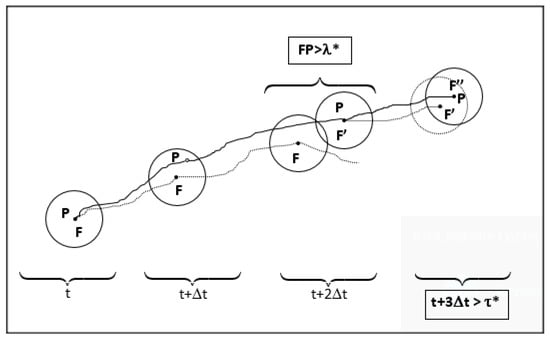
Figure 1.
Sketch of the eddy interaction model.
- the particle (P) leaves the fluid eddy (F) for entering into a new one when the eddy (F) lifetime is elapsed (condition 1),
- or when the distance between the particle and the eddy center does exceed the eddy length a radial dimension (condition 2).
The time step of the Monte-Carlo process will be, if condition 1 is verified, the eddy lifetime or, if condition 2 is respected, the transit time taken by the inertial particle to cover a distance larger than the eddy length , that is, The Monte-Carlo time is given by . Thus the eddy–particle interaction time is limited by the eddy lifetime or the transit time needed for the particle to cross the eddy. The eddy lifetime is related to a Lagrangian integral time scale or to a spectrum of the fluid turbulent flow, the eddy length to an Eulerian length scale of the turbulence. This kind of model should at least simulate part of the crossing-trajectory effects (CTEs), and, if possible, the inertia effects by solving the equation of motion with a time step . In the literature, the EIMs differ in the way the different time scales or length scales are chosen. In these stochastic trajectory models, the random fluid elements interacting with a particle have a length and time scales , and the fluid velocities can be generated with constant or random time steps . The velocity correlation functions are dependent on the choice of the type of time step probability density function as discussed by Wang and Stock [60]. In some cases, the Monte-Carlo process uses exponential distributions for the random eddy lifetime and size, with mean values equal to the Lagrangian integral time scale and to the Eulerian transverse length scale .
3.1.2. Historical Background
The basic ideas of a stochastic process for turbulent dispersion of particles were probably first proposed by Hutchinson et al. [61], and later by Brown and Hutchinson [62]. Eddies would be characterized by both a mean decay time and a “contact” time between an eddy and a particle, which could not exceed this decay time; a stochastic model simulated the random displacement of the particle colliding with eddies. Hotchkiss and Hirt [63] proposed a particle tracking scheme to simulate material transport with reference to a diffusion equation.
Later, Yuu et al. [64] assumed the particles would be trapped in successive energy-containing eddies without overshooting as in Tchen’s theory [43], each eddy having a constant lifetime and a random velocity fluctuation. Dukowicz [65] coupled a trajectory model to the SOLA code developed at Los Alamos by Hirt et al. [66] for liquid fuel sprays. The Monte-Carlo model was extended by Gosman and Ioannides [67,68]. The characteristic size of an eddy was set to the dissipation length scale and the eddy life time was where is an empirical constant of the turbulence model TEACH-T developed at Imperial College. The eddy interaction time is then given by where is the transit time. The eddy transit time can be easily obtained by a linearized equation of motion:
where is the slip velocity and the particle–eddy interaction time is therefore obtained classically by
It appears that the eddy interaction time for inertial particles cannot exceed the eddy lifetime, which is the fluid–particle interaction time or the eddy lifetime with an upper limit , the Lagrangian fluid integral scale. As a consequence, the heavy particle dispersion can never exceed the fluid–particle diffusion, a deficiency of most of the EIMs.
This method was then extensively used by Shuen et al. [69,70,71,72,73] for confined monodisperse particle-laden jets and non-evaporating and evaporating sprays, by choosing rather than , and they tuned their model to the diffusion theory in HIST and Snyder and Lumley’s experiment [15].
Chen and Crowe [74] simulated the experiment in a pipe flow of Arnason [75,76] and for the near isotropic homogeneous grid turbulence in Snyder and Lumley’s experiments [15]; however they calibrated the model by changing the constant to fit the last experiment. Durst et al. [77] developed a simple EIM based on the previous work of Gosman and Ioannides [67,68], and the equation of motion was solved analytically for short time steps. Milojevic [78] optimized the model for various test flow configurations [15,16,75,76]. It was modified for particulate two-phase systems with a size distribution by Sommerfeld and coworkers [79,80]. Mostafa et al. [81,82,83,84] coupled a model to the EIM to simulate experimental studies in turbulent evaporating sprays by optimizing the initial constants of the to functions. They used the relationship . Govan et al. [85] developed a simplified EIM to simulate their experiments in gas–solid pipe flows.
Ormancey and Martinon [86,87] proposed a 2-D model and introduced a procedure in order to calculate the fluid velocity at the particle position, taking into account a space correlation based on Frenkiel’s functions [88]. A relevant constant time step has to be used to numerically solve the equation of motion by a classical time discretization of the ODE’s. To account for the Lagrangian time correlations, eddy lifetimes are sampled according to a Poisson process. A variable y is sampled with a uniform probability density on [0, 1] and for each time step, two cases are possible. If , the random fluid velocity is kept constant. If , a new fluid velocity is generated, according to a Gaussian probability-density function. Then a Frenkiel space correlation is used and a Eulerian step is added to make a space correction to to obtain the fluid velocity at the particle position, where r is the distance between the particle (P) and the eddy (F) at time t. This fluid velocity is sampled according to a Gaussian probability-density function with
In the case where , it can be demonstrated that the process obeys an exponential fluid correlation function: .
The procedure can be divided into three steps,
- a first estimate of the fluid velocity with the criteria ,
- a spatial step that calculates the fluid–particle velocity at time at with a correlation function:
- the integration of the equation of motion with and to obtain the new discrete particle velocity.
Part of this method was used later by Hajji et al. [89] and compared to a spectral direct simulation model for heavy particles in HIST; nonlinear drag was also investigated for large Stokes numbers with drift velocity.
In some cases, the Monte-Carlo process used exponential distributions of the random eddy lifetime and size, with their mean values equal to the Lagrangian integral time scale and to the Eulerian transverse length scale . Kallio and Reeks [90] modeled particle deposition in an inhomogeneous boundary layer with random time scales drawn from an exponential probability density function (PDF). Burnage et al. [91,92,93,94] proposed an EIM based on Poisson and exponential distributions for the random eddy lifetime and size.
Most complete papers on the eddy interaction models and characteristics of the associated Monte-Carlo process are those written by Wang and Stock [18,19,20] and Graham [11,95,96,97] with mathematical arguments to clear the problem of self-consistency as pointed out by Kallio and Reeks [90], but also to make a real distinction between the standard eddy lifetime also defined as the fluid–particle interaction time by Graham, and a maximum interaction time , which can be randomly sampled, too [97]. is independent of and its choice determines a relationship between the turbulence structure parameter and the ratio of the Lagrangian and Eulerian integral time scale . It enables finite-inertia particles to disperse faster than fluid particles. Clearly, the particle–eddy interaction time is given by
where the factor 2 holds for self-consistency.
Wang and Stock [60] analyzed the relationships between different time step probability density functions , their mean value T and the Lagrangian integral fluid correlation time Graham [95,96,97] investigated the performance of the EIM in several of his papers and proposed enhancements in order to take into account the three effects, CTE, inertia and continuity, in inhomogeneous flows. He completed the study of Wang and Stock [5] and provided relations between the EIM, Lagrangian autocorrelations and Eulerian (fixed-point) correlations. These improved EIMs predicted that inertia effects without gravity can in some cases increase the long time dispersion of heavy particles, as was already obtained theoretically by Reeks [40] and Pismen-Nir [57], by the experiment of Wells and Stock [16] or by DNS [98] or LES [99]. The best agreement was obtained with the analytical results of Reeks in HIST.
Deutsch and Simonin [99] proposed the following formulas for the vertical and transverse components,
for the gravity direction, and
for the lateral case,
with , including CTE and CE but no inertia effect, since is not the fluid Lagrangian time along the discrete particle path without gravity.
Furthermore, Graham [97] extended his work to random length and time scales, with valuable results for non-homogeneous flows. Chen and Pereira [100] tested the Graham model; Chen [101] used the Graham/Gosman–Ioannides EIM for inhomogeneous anisotropic turbulence obtained by a Reynolds stress model and studied the inertia effects.
The advantage of the EIMs is that no time or space correlation has to be introduced in order to obtain the fluid velocity at the particle position. However, it is necessary to provide a time and length scale to characterize the interacting eddies. However, the method used for the time step or the eddy lifetime of the EIM, the time step probability density functions , is related to the form of the Lagrangian fluid autocorrelation and . Thus, with a PDF function an exponential function is obtained.
All the proposed models generally link the eddy characteristics (lifetime, size) to the turbulent kinetic energy and the dissipation rate and the Lagrangian and Eulerian scales with help of constants.
The constants A and B are adjusted to let the models simulate the classical test cases [102]. However, the method fixing the time step of the EIM, the time step probability density functions , is related to the form of the Lagrangian fluid autocorrelation and to the integral time scale . For instance, the way the constants are calibrated to fit a specific experiment is questionable, since they will in fact fix a virtual constant . The corresponding time scale, , will not be the Lagrangian fluid integral scale of a fluid particle but the effective Lagrangian fluid integral scale of a discrete particle along its trajectory. In that case the model will be optimized anyway to fit the simulation of the experimental test case.
Another advantage is that the EIM can easily be implemented in Eulerian codes of turbulence, and they can give a first qualitative and even quantitative idea of the dispersion. An open question in the EIM still exists in case of time and length distributions: since physically it is expected to have a relation between eddy size and lifetime, a small lifetime is expected for small dissipative eddies. A relationship between eddy size and lifetime should exist; the eddy turnover time of a size l eddy can be related to the time it takes for that size eddy to be reduced to the Kolmogorov scale, with an integral length scale L. Such relation should be
3.2. Random Walk Models (RWM-CWM)
Random walk models (or random flight models) are Lagrangian formulations based on Langevin’s equation. They have frequently been proposed to simulate the dispersion of pollutants in the atmosphere [103,104,105,106,107,108,109]. Several relevant reviews [7,12,109,110] make a critical analysis of these models, and several papers are more devoted to heavy particles [111,112,113,114,115,116]. Nevertheless, dispersion in the atmospheric boundary layer is not within the scope of this paper.
3.2.1. Classical Approach
The stochastic differential equation (SDE) modeling the behavior of fluid velocities in Gaussian turbulence, verifying Kolmogorov’s similarity theory for locally isotropic turbulence is
Langevin’s equation contains both a damping or drift term, which accounts for the friction exerted by the surrounding fluid on the heavy particle, and a random diffusion term, which models the fluid impulses, , being a Wiener white noise process, a stochastic process of zero mean and variance equal to the time interval . Equation (31) is the original Langevin equation for homogeneous stationary one-dimensional turbulent diffusion with no mean flow, and a Lagrangian correlation function . The discrete form of the Langevin’s equation (or Markov chain equation) correlates the fluid velocity fluctuation to its value at the previous step:
where is the rms value of the fluid velocity, is the Lagrangian autocorrelation and is a statistically independent, Gaussian, normalized and centered random number.
A classical Lagrangian autocorrelation function of the fluid velocity is simply given by this process:
is the time step and the Lagrangian integral time scale of the turbulence.
Note: For the simulation of the diffusion in a non-homogeneous turbulence, Equation (31) is not valid and Langevin’s equation including drift correction terms, as suggested by Legg and Raupach [108] must be used. This will be discussed in Section 5.
3.2.2. Two-Step Space–Time Approach
The extension of the Markov method to discrete particles has been proposed in many papers [117,118,119,120,121,122,123,124,125,126,127,128,129,130,131]. It was initiated by Zhuang et al. [117] following the EIM time–space method of Ormancey and Martinon [86,87].
The trajectory of fluid-discrete particle pairs is the elementary approach to model the fluid velocity seen by a discrete particle and is divided in two steps (Figure 2). Initially the fluid (F) and discrete (P) particles are at the same location at time t. and their respective velocities and are known. After a short time step they are located at and . The first step uses the discrete Langevin equation for the fluid element to estimate the eddy fluid velocity at and is a Lagrangian process in time:
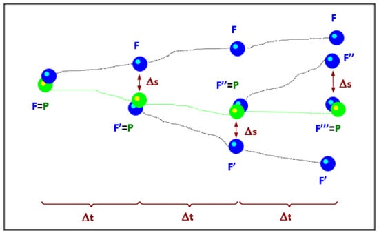
Figure 2.
Construction principle of an inertial particle trajectory in the random walk model (RWM).
The idea of the second step is based on the distance that separates the pair at time and uses a Eulerian space correlation coupled to the Langevin equation to obtain the fluid velocity at associated to a new fluid element (F’).
This value is used to solve the equation of motion and to calculate the velocity and the new position of the fluid element (F’) and of the discrete particle . A new fluid element is associated to the discrete particle at that new location. At each step a Cartesian frame is defined, with the origin at the fluid element position, and the first axis joins the inertial particle position to take into account the specificities of the directional correlation functions.
Then, a new fluid element (F’) is centered on the inertial particle (P), and the procedure begins again.
A combined two-step relation was first proposed for simplicity [117,118]. This version directly coupled the time and space correlations as
In case of a heavy particle with a mean fall velocity of , and a large drift parameter :
with , a Eulerian–Lagrangrian relationship [12,13]. This was suggested by Walklate [13] and can be compared to Csanady’s formulation:
Hunt and Nalpanis [119] suggested a different correlation function optimizing Snyder’s measurements [15]:
Simulations in HIST [120] with the above equation were performed for heavy particles and compared to other simulations obtained with a Frenkiel zero correlation (m = 0) and the theoretical results of Wang and Stock.
Furthermore, much effort was dedicated to anisotropic turbulence. Berlemont et al. [121,122,123] proposed a sophisticated formulation; it will be briefly discussed in Section 3.3 since it is a multistep random method. Zhou and Leschziner [124] introduced a temporal correlation approach taking into account anisotropic Lagrangian time scales, including directional and temporal correlation coefficients between and and the covariance matrix of . Burry and Bergeles [125] and Lu et al. [126,127,128,129,130] generalized the method to anisotropic flows, with temporal and spatial correlations, according to the anisotropy of the Reynolds stresses. Lu used a Eulerian velocity autocorrelation instead of a Lagrangian one, Mashayek [131] compared results obtained with Lu’s Eulerian stochastic model with the direct numerical simulation (DNS) data of Mei et al. [132].
The proposed models are related to complex generalized Langevin equations use relationships , relationships often similar to those of the EIMs,
or more complex correlation functions in case of tensors. As for the EIMs, the different constants are tuned to best simulate turbulent diffusion and other experiments and test cases, and are compared to DNS results.
Other papers have compared the performance of different Lagrangian stochastic models, too. For the Snyder and Lumley experiment [15], an extensive comparison of different EIM and RWM results obtained by Berlemont [122], Gosman and Ioannides [67,68], Ormancey and Martinon [86,87], Shuen et al. [69], Lu et al. [127], Nir and Pismen [57], and Meek and Jones [54] was proposed by Huilier et al. [133]. Apart the choice of the constants A, B or CT, some other factors can influence the simulations and justify discrepancies, the number of computed trajectories, the choice of the random number generator or the time step . Lain and Grillo [134] simulated the Wells and Stock experiment [16] and a jet flow [135].
Within the last two decades, research has been focused on enhancements of RWM and on the formulation of Lagrangian stochastic models and PDF models [131,136,137,138,139,140,141,142,143,144,145,146,147,148,149,150,151,152,153,154,155,156,157,158] for the transport of particles in more complex turbulent fields, and substantial work was also addressed on the spurious mean particle drift in inhomogeneous turbulence as introduced by McInnes and Bracco [102] or Legg and Raupach [108]. Zhou and Leschziner [136] presented more sophisticated models able to integrate directional/cross correlations (full correlation tensors or the directional correlations, and the anisotropy of turbulence scales). These models should be able to simulate the dispersion of particles in anisotropic turbulence, shear flows or boundary layers. It is not the intention of the present paper to detail these approaches, but some of these methods are summarized and discussed by Pozorski and Minier [139], Bocksell and Loth [142,149], Minier et al. [157] or Tanière and Arcen [158]. The models were also modified according to the true fluid velocity along a particle path and the classical fluid integral time scales where replaced by integral scales integrating inertia and gravity in relation with Csanady’s formulas (Section 2.2.4). Most models often used also the theoretical results by Wang and Stock developed in Appendix A.
3.3. CRW–Matrix Methods
Several models used multistep Markov chains, which is the fluid velocity along the trajectory of the discrete particle at time t is evaluated with more than one previous calculated velocity, that is
Berlemont et al. [121,122,123] were the first to propose a matrix method able to simulate the fluid velocity along a part of the trajectory for any time correlation function. The aim was to generate a sequence verifying Lagrangian Frenkiel family correlation functions and the stress tensor. At the same time for a given time step, a Eulerian correction was applied; once the distance between the two particles exceeded the lateral Eulerian scale, a new fluid particle was generated. However, the fluid–particle velocity field was that of a tracer, because related to the classical fluid–particle correlation, the Eulerian process should simulate the CTE and inertial effects. This kind of method can be classified as a hybrid RWM–matrix method since they use a multistep Markov chain simulation of the fluid–particle velocity.
In Berlemont’s formalism, the fluid–particle fluctuating velocities are given by
where the vector Y has uncorrelated variables with a Gaussian distribution and the matrix B is related to the Lagrangian time correlation tensor and a matrix A by
The set of equations can be rewritten as a generalized Langevin equation under matrix form
where the matrix M includes the effects of previous time steps, vector is sampled from Gaussian PDF, and the fluid velocity at the new particle position is then obtained with Frenkiel space correlation functions.
A matrix method, different from that earlier proposed by Berlemont et al., has been developed by the research group at Strasbourg University [159,160,161]. The idea is to generate a random sequence of fluid velocities for the whole trajectory. The time series algorithm is able to reproduce stochastically any fluctuating velocity field in HIST, at least if the autocorrelation tensor is known.
Starting with the following system, where at each time step, the fluid fluctuating velocity is a linear combination of random numbers, statistically independent, centered and normalized ξk with a Gaussian probability density function:
and by multiplying successively all the equations of the system with the first equation, and averaging the obtained products, we obtain:
This yields the first column of the low triangular matrix A. Then the initial set is multiplied by the second equation and so on, and the whole matrix A can be built. Matrix A is unique for each chosen Lagrangian autocorrelation. A given set of random numbers will represent a fluid velocity along a particle trajectory (indeed, a linear system has to be solved for each trajectory) and will be used to solve n times the momentum equation of motion. It is clear that for long time diffusion , this method requires computer resources since the dimension of the matrix will be . Nevertheless, correlation is typically lost after a time and the triangular matrix A can be replaced by a band matrix B (Figure 3), the terms of that matrix can be used to calculate the fluid velocity and the number of floating point operations will be reduced.
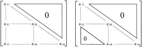
Figure 3.
Matrices A & B used to calculate the turbulent fluid velocity seen by the particle along its path.
Pétrissans et al. [162] later proposed a more effective model, less computer time-consuming, based on different time series, an autoregressive–moving-average ARMA (2,1) process, using a second-order time series and a first moving average. The model was able to generate the Wang and Stock’s Lagrangian correlation functions and predicted the effect of negative loops.
3.4. Numerical Context
Most of the Lagrangian models, among which are either EIM or RWM, use experimental data or test flows to verify their ability and performance to simulate turbulent dispersion. First of all, they must be able to simulate turbulent diffusion in homogeneous isotropic turbulence as predicted by the analysis of Taylor; furthermore, they are generally tested and optimized to predict the dispersion of particles or droplets in various configurations, grid turbulent flows [15,16], horizontal or vertical pipe flows [17,75,76,163,164,165,166], round jets [84,167,168,169,170,171,172] or in mixing shear layers [173]. Last, they are often used to simulate the dispersion in HIST, and their performance is tested on theoretical or numerical results obtained by other techniques. One of the aims of the present paper is to verify if these methods can take into account the inertia and gravity effects.
Concerning the flow and particle properties in HIST, we focus on the impact of inertia and drift effects governing the dispersion of spherical particles, with a density of = 1000 kg/m3 and a diameter d in the range of 10 to 500 microns. The spheres are released from a point source and disperse in a homogeneous isotropic stationary turbulence (HIST), the fluid flow being air under standard conditions (density = 1.275 kg/m3 and kinematic viscosity = 1.36 × 10⁻⁵ m/s2) without gravity and a gravity field. The scale of the turbulent fluid is = 0.131 m/s and the Lagrangian integral time scale is set to = 0.091 s. The experimental data by Sato and Yamamoto [174] suggested that for a grid turbulence where is the moving Eulerian integral time scale. Burnage and Huilier [175] performed a diffusion experiment with small droplets released isokinetically from a tube in a grid decaying turbulence, using LDA and a light diffusion technique to measure the turbulence and concentration field and found [13]. In the present study, we suppose that (Appendix A). As a consequence, in the present simulations, the Stokes number, , will range from 0.007 to 4.4, being the Stokesian particle relaxation time (details are summarized in Table 2). All the statistics that will characterize the particulate dispersion, namely, turbulent energies (variances) , Lagrangian particle integral time scales and long time particle dispersion coefficients , are calculated for 50,000 trajectories for each particle size (Stokes number), a number of trajectories sufficient to ensure statistical stability and convergence.
Table 2.
Particle properties and dimensionless control parameters.
The equations of motion as simplified for heavier particles (section equation X) are solved numerically by a fourth order Runge–Kutta algorithm, and the time step is set from 10−4 s to 10−3 s with particle relaxation times from 1.2 × 10⁻³ s (d = 20 µm) to 0.8 s (d = 500 µm).
The drift parameter due to gravity g = 9.8 m/s2 varies from 0.02 for the smallest particles to 15 for the largest. The long time dispersion characteristics are calculated for 4 s trajectories, a time that largely exceeds by a factor of 5 to 10 the particle relaxation time of the heavier particles and the Lagrangian scales. Besides other tests on nonstationary forces (added mass, Basset term), lift forces confirmed that statistically there is no influence on long time dispersion of heavy particles [93], in agreement with other results in the literature.
4. Numerical Results
4.1. EIM–DRW Results
We consider here an extension of the EIM initiated by Burnage and Moon [91] and furthermore developed by Huilier et al. [93,133,175,176,177]. The eddy lifetime and the eddy length are distributed randomly according to exponential probability distribution functions with average values respectively equal to the fluid Lagrangian integral time scale in Section 4.1.1 and to the Lagrangian time proposed by Wang and Stock in the Appendix A in Section 4.1.2; for the length scale related to the eddy lifetime, the transverse Eulerian integral length scale was used. The instantaneous fluid eddy’s velocity was given by the sum of a mean and a fluctuating velocity. Each component of the fluctuating velocity was evaluated from a Gaussian probability distribution with zero mean and a variance equal to , the rms value being also called “the eddy velocity scale.” In this study, the assumption is made that during the interaction between an eddy and the particle, the fluctuating fluid velocity remains constant. Besides, it is supposed that the particle stays in a same fluid eddy as long as:
- (1)
- the distance between the eddy center and the heavy particle position does not exceed the random eddy length (no overshooting condition),
- (2)
- the interaction time of the particle does not exceed the random eddy lifetime.
If either of these two conditions becomes invalid, the heavy particle will be centered on a new random fluid eddy.
4.1.1. Classical Dispersion Without Gravity (g = 0)
Without any external force field (no gravity, g = 0), one can reasonably assume that the particle Reynolds number is less than one, since the mean fluid–particle slip velocity is zero. In that case, the drag law is linear (Stokesian, f = 1). All classical EIMs consider that the turbulence along a particle path has as Lagrangian time scale. Only inertial effects have to be taken into account with no gravity term, although crossing-trajectory effects cannot be excluded since due to inertia particles can cross small eddies rapidly. The general trend is that as expected, the turbulent particle integral scale increases with the Stokes number (Figure 4) and particle turbulence decreases with inertia (Figure 5). But very inertial (heavy) particles disperse much less than fluid elements (Figure 6), the dispersion coefficients being normalized by the fluid diffusion coefficient equal to . This is in contradiction with now well recognized results, either theoretical [52] or numerical results (obtained by direct or large eddy simulations). In conclusion, the inertial effect is not well simulated by this type of model based on . Simulations were performed with the same model without overshooting [176], they simply verified Tchen’s theory, which is obsolete for heavy particles since crossing-trajectory effects are not considered.
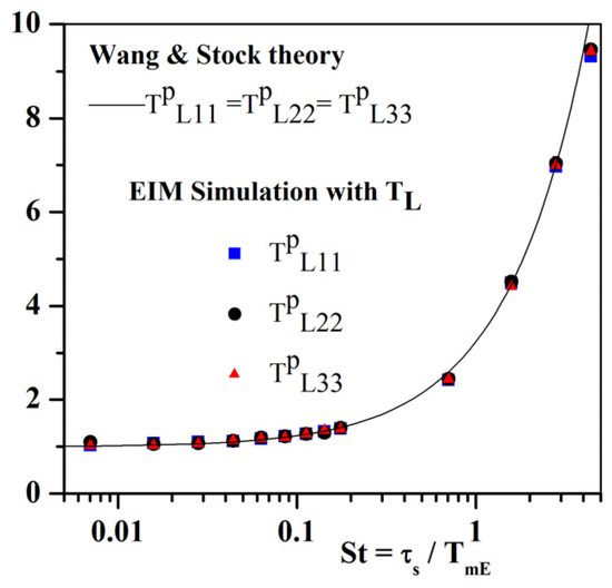
Figure 4.
Particle Lagrangian time scale (g = 0).
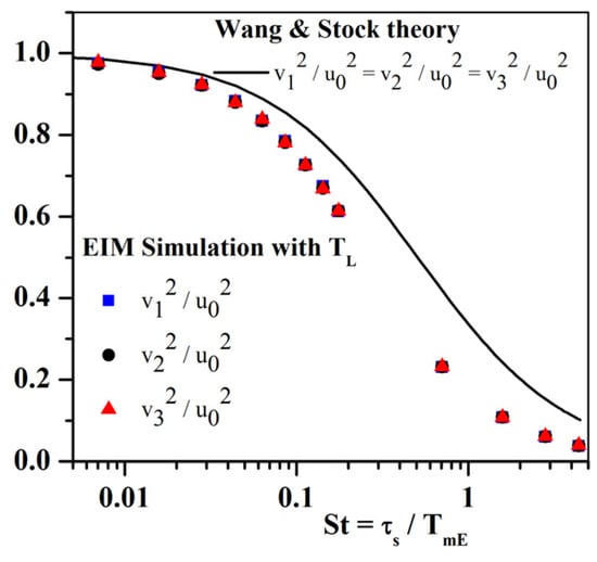
Figure 5.
Normalized variance of particle velocity (g = 0).
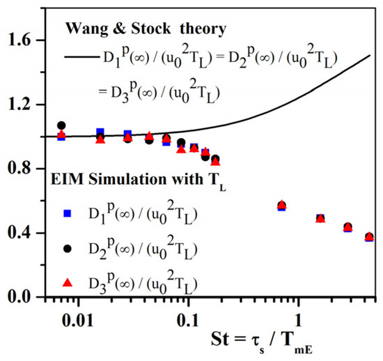
Figure 6.
Particle dispersion coefficient (g = 0).
4.1.2. Modified EIM with Wang and Stock Correction (No Gravity)
A similar simulation but with Wang and Stock’s relation (Equation (A1) in Appendix A) gave much more promising results for the turbulent energies (Figure 7). In particular, Figure 8 indicates that the ratio of the particle dispersion coefficient to the fluid diffusivity is greater than unity for the large Stokes number; this result is in accordance with the theories of Reeks [40] or Pismen and Nir [57], with the experimental observations of Wells and Stock [16], with the direct numerical simulation of Squires and Eaton [98] and with the large eddy simulation of Deutsch [178]. Only for large Stokes numbers are the particle dispersion coefficients underestimated; this is due to the effects of nonlinear drag on the Lagrangian particle integral time scale and the particle velocity scales [176]. Comparisons between results obtained with Stokes’ drag and nonlinear drag were also proposed by Wang and Stock [6] and also showed an increase of the velocity variance with use of the nonlinear drag mainly due to the difference between the Stokesian relaxation times (and so the related Stokes number) being larger than the nonlinear terms when the particle Reynolds number (Table 2).
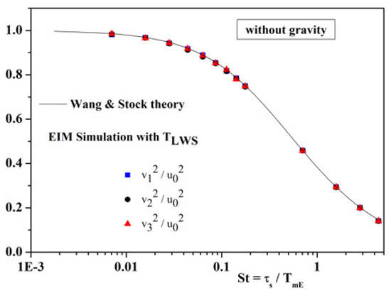
Figure 7.
Normalized variance of particle velocity (g = 0).
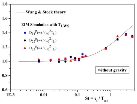
Figure 8.
Particle dispersion coefficient (g = 0).
4.1.3. Dispersion under Gravity Effect
Fluid-particle slip velocity under gravity can be non-negligible for heavy particles, so that the particle Reynolds number can be much larger than 1 and a non-Stokesian drag law must be used, since the fall velocity increases with particle size. In the present case, a drag law given by Schiller and Naumann [37] was proposed. This law is generally accepted, as other laws bring no real modifications. The present results consider again that the heavy particle is controlled by a fluid Lagrangian scale equal to . Although the influence of the time step and number of total trajectories on the results was investigated, the results are mixed and scattered for the larger Stokes numbers at least for the time scales (Figure 9) and the particle dispersion coefficients (Figure 10). The normalized variances of the particle velocity fluctuations (Figure 11) and the dispersion coefficients are overestimated for the larger Stokes numbers (heavy particles) although decreasing as predicted by Wang and Stock’s theory, even if the decrease is induced by the overshooting (crossing-trajectory) and inertia. But the continuity effect is not restored.
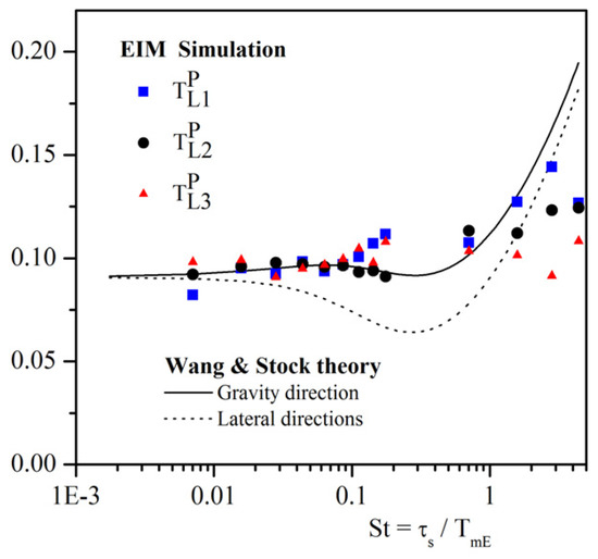
Figure 9.
Particle Lagrangian time scale (g ≠ 0).
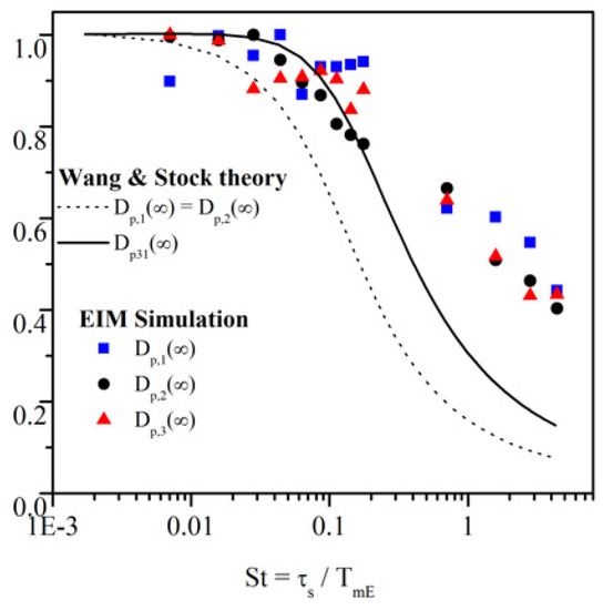
Figure 10.
Particle dispersion coefficient (g ≠ 0).
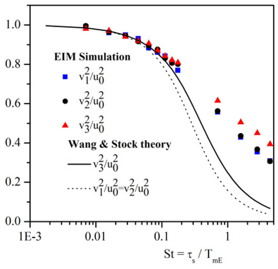
Figure 11.
Normalized variance of particle velocity (g ≠ 0).
4.1.4. Conclusion on EIM–DRW Monte-Carlo Methods
It is a matter of fact that Lagrangian numerical simulations based on EIM–Monte-Carlo processes cannot predict the dispersion of heavy particles with or without gravity. The shortcomings of the method are due to the fact that the heavy particle will interact with an eddy during a given time, the maximum of which is normally the eddy life (taken as the Lagrangian scale TL). Major modifications were brought to Monte-Carlo approaches by Huang et al. [179], Graham [95,96,97], Launay et al. [176,177], among others, and some eddy–particle interaction models tried to better take into account the space–time characteristics of the effective fluid turbulence controlling the particle motion, to better simulate the so-called “true turbulence experienced by the particle’.”
The weakness of the EIM–DRW method is that the correlation functions and Lagrangian integral time scales are related to the way the time step or eddy lifetime is chosen [5,60]. Furthermore, the eddy length and lifetime are not correlated, so that no turbulence spectrum is really simulated. In addition, the different models proposed are generally tested on well-known flow cases [18,19] and optimized by calibrating a few parameters. Several papers compared different EIMs [120,133] and showed that even for these test cases, some EIM approaches are deficient and the differences in the numerical results are tremendous. It follows that EIM–DRW models are certainly not appropriate to more complex gas–solid flows, shear flows, anisotropic flows, since even in case of HIST deficiencies have been observed. That is why scientists have focused more and more of their research on Markovian methods for two decades.
4.2. Markovian Methods
We consider here the models as defined in Section 3.2 and two kinds of simulations will be presented here:
- The Markovian model developed by a two-step space–time approach (Section 3.2.2) with the following equations and the method proposed by Lu et al. [126,127,128,129,130]:where are normalized Gaussian random numbers.
- A more classical Markovian model with a Langevin equation based on the correlation functions proposed by Wang and Stock (Equation (A2)):
4.2.1. CRW–Lu Model
In the 1990’s it seemed that a modified EIM influenced by a Markov chain model could bring some progress. That is why a space–time Langevin equation was explored. The idea was to couple Eulerian space correlations to Lagrangian time correlations; the idea was not so bad and was explored with some hope and used to simulate grid turbulence experiments [15,16]. The method as proposed by Lu et al. [126,127,128,129,130] was applied to HIST, but gave poor results. Without gravity and for small particles, which behave like small inertial particles, the particle Lagrangian time was 15% less than the Lagrangian fluid integral time . All possible parameters, among them the time increment , were changed and gave no better results. Presently, simulations with this model are still being undertaken. The particle variance seems to yield results similar to an EIM based on . It is clear that the effect on underestimating the particle dispersion is directly related to the integral time scales, and the space correction is certainly not valid, even if the approach gives satisfactory results for grid turbulence experiments, due to calibration of constants related to turbulent kinetic energy and dissipation. As for many models it is now clear that just simulating these experiments and modifying them for anisotropic flows is not the best choice.
- Dispersion without gravity (g = 0)
As shown in Figure 12, the normalized variances of the fluctuating velocity of the particles are generally underestimated, except for the smaller Stokes numbers (less inertial particles). The same holds for the Lagrangian integral time scales (Figure 13) as well as for the normalized dispersion coefficients (Figure 14). Thus, the model based on Markovian chains is not suitable since the inertial effect (IE) of the particles cannot be correctly simulated.
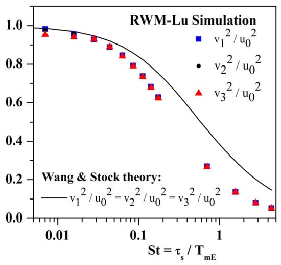
Figure 12.
Normalized variance of particle velocity (g = 0).
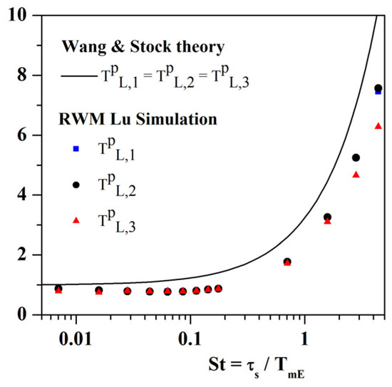
Figure 13.
Particle Lagrangian time scale (g = 0).
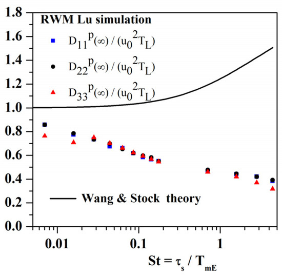
Figure 14.
Particle Dispersion coefficient (g = 0).
- RWM–Lu with gravity effects (g ≠ 0)
The turbulent energy of the heavy particles is well predicted by the model except for intermediate Stokes numbers, where it is somewhat underestimated (Figure 15). One can note that overall, this model yields better results for the particle turbulent energy than those obtained by an EIM–Monte-Carlo model (Figure 11). Again, long time dispersion coefficients are systematically much smaller (up to a factor of 2) than Wang and Stock theory for the smaller Stokes numbers (Figure 16). They decrease with larger particle inertia and for larger Stokes numbers, the ratio of transverse to gravity direction dispersion coefficients is close to a value of 0.5 in accordance with Csanady’s early results [42]. Such a Markovian model seems to be able, at least partially, to simulate effects of crossing trajectories and continuity, but the estimates of the dispersion coefficients are significantly small.
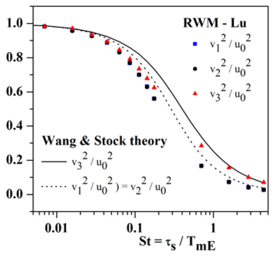
Figure 15.
Normalized variance of particle velocity (g ≠ 0).
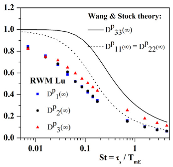
Figure 16.
Particle dispersion coefficients (g ≠ 0).
4.2.2. Langevin-WS Model
The Langevin model based on the Wang and Stock correlation functions seems more promising. Without gravity, this model gave results close to the theory of Wang and Stock, in accordance with results presented for the EIM in Section 4.1.2. We present here only the simulations with the gravity–CTE-CE effects (Figure 17, Figure 18 and Figure 19). The following equation is used with correlation functions given by Equation (A2):
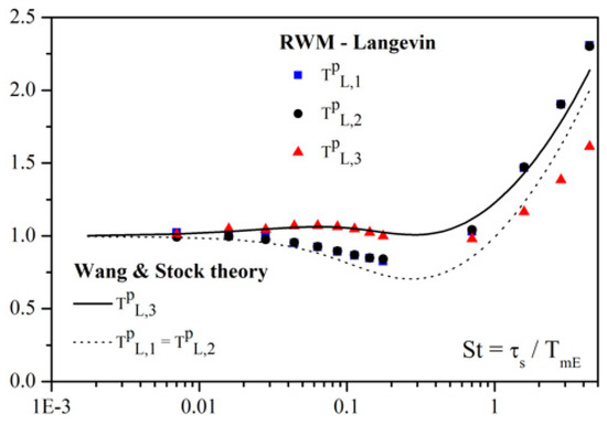
Figure 17.
Particle Lagrangian time scale (g ≠ 0).
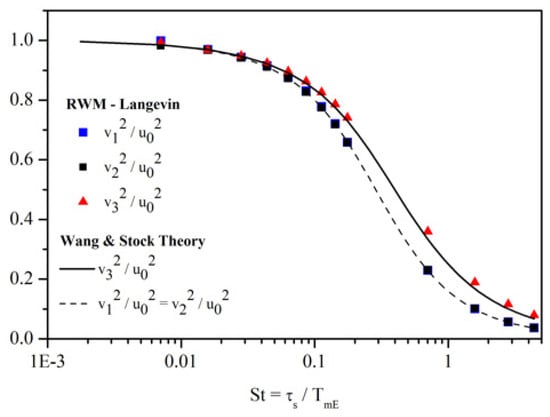
Figure 18.
Normalized variance of particle velocity (g ≠ 0).
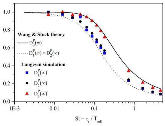
Figure 19.
Particle dispersion coefficient (g ≠ 0).
It is clear that this model is efficient, but in other models as well as the last, which will be presented in Section 4.3, the support is conditioned to an appropriate relationship of the correlation functions to the Stokes number and the drift parameter, in this case the Wang and Stock model detailed in Appendix A. The influence of the time step was not investigated but was always less than 1/10 of the typical time scales .
4.2.3. Conclusions on Markovian Models
The prediction of the dispersion of heavy particles, based on Markov one-chain Lagrangian models, seems encouraging. Two of the three main effects, crossing-trajectory and continuity, are rather well reproduced, except for the inertial effect, which enables particles under zero gravity to disperse more than fluid elements, a result obtained theoretically by Reeks [40], for instance. Furthermore, the long time dispersion coefficients are under-predicted both with and without gravity effects. Nevertheless, Huilier [120], on the basis of Launay’s thesis [159] and complementary simulations, clearly showed in a previous paper the important influence of various autocorrelation functions [20,23,24,120] on the dispersion coefficients of heavy particles and one-step Markovian simulations with adequate autocorrelations can bring enhanced results.
4.3. Matrix Method and Related Considerations
The matrix method proposed by Launay has no real obvious gap, it is a statistical method based on any correlation function and therefore simulates the fluid velocity along the path of a discrete particle if the function is known. The following results are of course in agreement with the Wang and Stock theory. The main problem persists with large Stokes numbers because it is not obvious that the Wang and Stock theory is guaranteed by such large Stokes numbers.
4.3.1. Matrix Method without Gravity (g = 0)
In order to check that the proposed Lagrangian method also correctly restores the inertia effect (increased diffusivity of high-inertia particles), the dispersion of particles without any drift velocity was first studied. In this case the parameter f was taken as one in the Equation (9), id linear drag. The matrix model is self-consistent, in accordance with the model proposed by Wang and Stock, for the particle Lagrangian integral time scales (Figure 20) and the particle turbulence (Figure 21). Again, as in Section 4.1.2 with the modified EIM, previous theoretical works (Reeks [40], Pismen and Nir [57]), experiments (Wells and Stock [16]) and numerical studies (Squires and Eaton [98], Deutsch [178], Graham [96,97]) are confirmed for heavy particles with large inertia that disperse faster than the fluid elements. Figure 22 shows that the ratio of the particle to the fluid dispersion () coefficients is greater than unity for large Stokes numbers: this indicates that the inertia effect is well taken into account by the proposed method for predicting the turbulent dispersion of the heavy particles. The drop-off for Stokes numbers larger than 3 (last point in Figure 22) was never explained up to now; in fact, referring to Launay [159], the particle integral time scale is under-predicted, although the particle turbulence is in accordance with the theory of Wang and Stock. Either a non-linear drag for these very inertial particles should be considered; but calculations based on a Monte-Carlo and a non-linear drag law also underestimated the theoretical values for Stokes numbers larger than 3 as shown by Matt and Huilier [180]. Trajectory calculations over a longer path time (typically ) should then give better results.
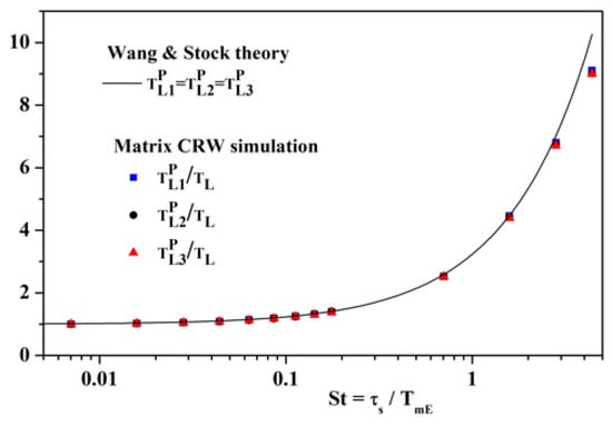
Figure 20.
Particle Lagrangian time scale (g = 0).
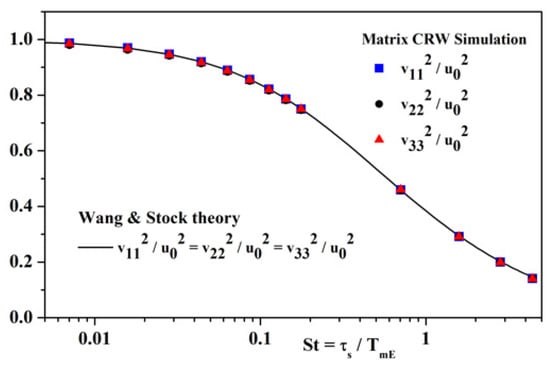
Figure 21.
Normalized variance of particle velocity (g = 0).
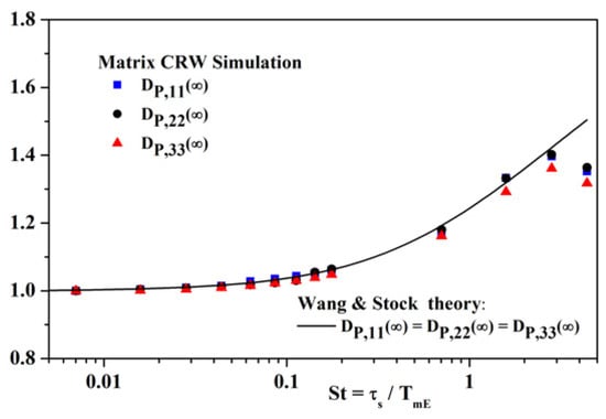
Figure 22.
Particle dispersion coefficient (g = 0).
4.3.2. Matrix Method with Gravity (g ≠ 0)
Figure 23, Figure 24 and Figure 25 yield the numerical results obtained with the proposed Lagrangian model. The whole of the numerical results is again compared with the theory developed by Wang and Stock. In Figure 25, the analytical and calculated long time dispersion particle’s coefficients decrease with the Stokes number St in free-fall direction (direction 3) as well as in the two directions orthogonal to the free-fall direction (directions 1 and 2). The agreement between the numerical simulations and the theoretical expressions is very good and the effect of crossing trajectories and continuity effects is clearly seen. Besides, it is shown in Figure 25 that the particle’s dispersion in the free-fall direction is larger than in the two transverse directions by a factor close to 2.
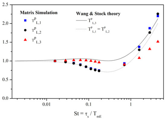
Figure 23.
Particle Lagrangian time scale (g ≠ 0).
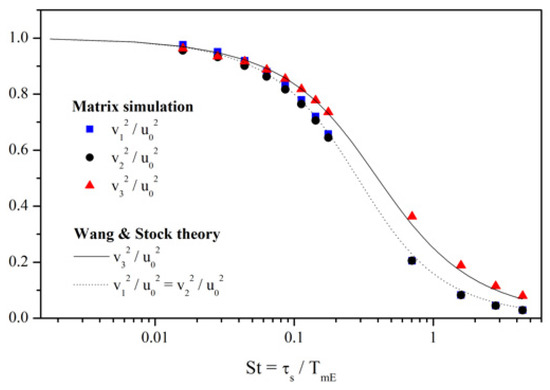
Figure 24.
Normalized variance of particle velocity (g ≠ 0).
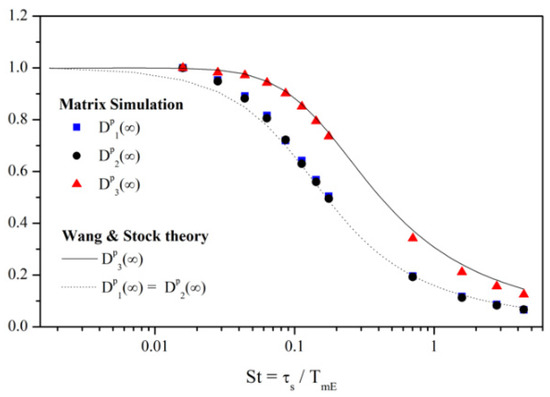
Figure 25.
Particle dispersion coefficients (g ≠ 0).
5. Discussion and Present Trends of Modeling Approaches
The present study only gave an overview of the relative performance of Lagrangian particle tracking methods for the turbulent gas–particle transport in HIST. The EIM was historically extensively summarized, the RWM partly. The main advantage of these methods is that they help to better understand the mechanisms and concepts of inertia and crossing-trajectory effects. Although presenting some other advantages, a crucial disadvantage is that these methods require many trajectory calculations to achieve statistical convergence.
The EIM, sometimes also called ELT (Eddy Life Time), is often coupled to k-eps or RANS turbulence models, is easy to implement and gives a first idea of the influence of inertia and gravity on the behavior of discrete particles in interaction with turbulent structures. But it seems, as demonstrated, that EIM hardly can predict accurate behavior of heavy particles in HIST and certainly not in complex flow configurations, although these methods were extensively applied to polydisperse sprays in combustion.
Markovian methods using time and space correlations are still discontinuous random walk methods, and they have been developed as a possible improvement of the EIM methods. Mainly the experiments by Snyder and Lumley [15] and Wells and Stock [16] served as test cases to optimize these models and calibrate some constants. As shown in Section 4.2, they were not able to simulate correctly turbulent dispersion in HIST, too.
The meteorology community working on air pollution and turbulent diffusion in the atmosphere certainly brought a decisive contribution. A major effort was devoted to optimize DRW and CRW models in inhomogeneous turbulence with the help of the Langevin equation. Initially the Langevin equation was used to model the Brownian velocity fluctuations. The stochastic equation was then applied to homogeneous turbulence by Obukhov [181] in terms of a Fokker–Plank equation related to a Gaussian probability distribution [182,183]. The CRW-Langevin equation first served to model turbulent dispersion in the tracer limit, when particles are considered as passive contaminants or fluid elements. In homogeneous stationary one-dimensional Gaussian turbulence the Langevin equation reduces to equation
When applied to inhomogeneous flow, such as in boundary or shear layers, the classical models, among which is the original Langevin equation, predict that particles migrate from regions of high turbulence intensity (core or bulk region) to the regions where the intensity is minimum (wall) and those even in the tracer limit. This is due to the sampling of fluctuation velocity, inducing a spurious drift component of the mean flow and introducing an unphysical accumulation and deposition velocity into the wall regions.
Early Wilson et al. [184,185] proposed a correction related to the effect of turbulent acceleration of the particles for the vertical velocity component , in terms of a vertical bias velocity added to the RHS of the Langevin equation, being the root-mean square of the vertical velocity. Several papers [186,187] refer to a problem of consistency between the classical Langevin equation and the equations of the mean flow field when particles are so small that they behave like fluid eddies. Classical models do not obey the well-mixed criterion as defined by Thomson [7], that is: “A tracer field which is initially well mixed in an inhomogeneous turbulent field should remain well mixed”.
The spurious drift term is related to the fluid acceleration
with
by averaging
The second term is non-zero in case of inhomogeneous turbulence, and the drift correction velocity is then given by
in the tracer limit. In case of inertial particles, Bocksell and Loth [149] proposed a spurious drift correction given by
so that the classical Langevin equation with spurious drift correction reads:
an equation that meets the well-mixed condition and can be reasonably used except in strongly inhomogeneous turbulent flows such as boundary layers. More generally, a generalized Langevin equation model, as proposed by Haworth and Pope [188], was developed and is in active use. Pope [189] initially established PDF methods for reactive flows. He also fixed the consistency conditions [190]. Several simplified versions exist [191] and one simplified equation is
Numerous studies have been proposed to improve stochastic Lagrangian models derived from the generalized Langevin equation, related to PDF approaches of the fluid velocity, such as the models initially developed by Simonin et al. [192], Minier and coworkers [157,193,194,195,196,197], Reeks [40,198,199,200,201,202] or Tanière and coworkers [151,152,153,158]; they first focused on different expressions of the drift vector. Reeks extensively worked out a kinetic equation in relationship to the generalized Langevin model (GLM) probability density function (PDF) equation. “Should the kinetic equation be ill-posed?” was mathematically discussed by Minier and Profeta [203] and Reeks et al. [204]. The most recent paper on kinetic equations was given by Zhong et al. [205].
From a scientific point of view, RANS methods have been progressively replaced by more accurate methods (LES, DNS), even if the computational cost is higher. With the progress in computer performance, the Eulerian–Lagrangian models and particle tracking methods have focused progressively on a large eddy simulation (LES), coupled to stochastic particle subgrid scale (SGS) models, proposing Langevin equations for the fluid seen along the heavy particle trajectory in order to solve the momentum equation for particle-laden flows [206,207,208,209,210,211,212,213,214,215,216,217,218,219,220,221,222,223,224,225,226].
One of the more detailed particle SGS models is that proposed by Berrouk et al. [209,210,211], based on the Wang and Stock equations (Appendix A), integrating inertia, CTE, continuity and anisotropy; the filtered fluid field is calculated by an LES closed by a classical fluid SGS model, and the fluid velocity seen by the particle is obtained by a Langevin equation solved by a first-order Euler scheme; the Langevin equation is given by
Continuity, CTE and inertia appear in the drift term. is related to the Lagrangian time scale of the subgrid fluctuations with the Wang and Stock correction for inertia and Csanady’s expressions for mean drift and transverse directions in case of gravity. More details are given in Berrouk et al. [210] (pp. 8–10) for the closure of the drift and diffusion terms, the last being modified for anisotropy and non-stationarity through a diagonal, non-isotropic diffusion matrix . Both parameters depend on the ratio between the Lagrangian and Eulerian time scales or , which was kept constant in all the studies proposed by Wang and Stock [18,19,20] and equal to 0.356, referring to a turbulence structure parameter m equal to 1 (Appendix A). The model was used to simulate the dispersion experiments of Arnason in a pipe flow [75,76]. Nevertheless, as mentioned, the normalized time scale or the Kolmogorov constant varies considerably as given in the literature [9,10]. Last, a main persisting problem is related to the choice of the value of the turbulence structure parameter .
Several benchmark tests exist and LES results are sometimes compared to DNS models, which normally provide exact numerical flow fields, to evaluate the predictive capability of particle dispersion in more complex turbulent flows. For instance, an international benchmark [227] was proposed for LES Eulerian–Lagrangian simulations in a particle-laden channel flow, gathering a large database, and was compared to DNS results. Marchioli [228] recently presented a review of LES in turbulent dispersed flows, which was complementary to other reviews and guidelines [157,197]. Objectives at least should be able to model physical mechanisms such as erosion or deposition, settling, saltation of aerosols or solid particles in bounded flows, migration in shear layers and boundary layers, preferential concentration and turbophoresis. Particles tend to segregate in decreasing turbulence level region wall areas, and the rate of deposition is enhanced on surfaces. Caporaloni et al. [229] and Reeks [230] independently called this phenomenon “Turbophoresis,” analogous to the thermophoresis or Ludwig–Soret effects. Furthermore, dense particles tend to accumulate and cluster in specific convergence regions and are centrifuged away from vortex zones. The influence of coherent vortex structures on particle dispersion was recognized early by Crowe et al. [231,232,233], Chein and Chung [234], and studied by Eaton and coworkers [235,236,237,238,239] as well as the research group of Cartellier or Bourgoin [240,241,242,243,244,245,246,247], among others. Preferential concentration has since been extensively reported in the literature during the last two decades, and the physical clustering mechanisms have been identified, namely, sweep-stick, heavy particles migrating to low acceleration regions [248,249] and centrifugal expulsion effects, inertial particles accumulating in low-vorticity zones of the carrier flow.
To conclude, other review papers on modeling particle-laden flows or multiphase flows are of interest [250,251,252,253,254,255,256,257], including, in some cases, collision and turbulence modification by particles in dense gas–particle flows. Some general and complete reviews should be mentioned, too; the relevant review by Balachandar and Eaton [258] on different aspects of turbulent dispersed multiphase flows focusing on preferential concentration and different coupling mechanisms (e.g., interphase, two-way momentum coupling, turbulence modulation), and a general review of Lagrangian statistical properties of particles by Toshi and Bodenschatz [259].
Furthermore, aside from the interest brought in the literature to single particle Lagrangian structure functions, with comparison between experiments and DNS instance, e.g., [260], turbulent diffusion and dispersion have also been investigated in terms of the mean-square displacement of a pair of particles relative to their center of mass and relative velocity between pairs. Relative or particle pairs dispersion has been, since the pioneering paper by Richardson [261] and Batchelor [262], extensively studied theoretically, experimentally and numerically, in relation to new stochastic models and DNS calculations [263] or experiments [264,265]. Significant reviews on turbulent relative dispersion were those of Sawford [266] on two-particle Lagrangian stochastic models, Salazar and Collins [267] on more recent advances. The reviews are often related to tracer diffusion and HIST, and offer an increased understanding of the Lagrangian properties of turbulent flows. But they as well as other articles not only concern low-inertia particle pairs [268] but also separation of high-inertia particle pairs [269,270] and preferential concentration [271]. A new review on turbulent relative dispersion studies would be welcome.
Funding
This research received no external funding.
Data Availability Statement
The data presented in this study are available on request from the corresponding author.
Acknowledgments
In memoriam, the author expresses his great thanks to Emeritus David E. Stock from Washington State University for his encouragement to promote teaching Fluid Mechanics and Multiphase flows in France and to humbly contribute to research in these scientific fields.
Conflicts of Interest
The author declares no conflict of interest.
Appendix A
Wang and Stock’s work on their model in HIST was summarized in several papers [18,19,20,60] and an ASME lecture by Stock [257]. Wang and Stock [18] established an analytical approximation for Gaussian turbulence that concludes that is always less than 1 but depends on the structure parameter , the ratio of the moving Eulerian scale to the eddy turnover time . Using a numerical simulation generated by Fourier modes, Wang and Stock [20] proposed a relation for the fluid time scale seen by a heavy particle with zero drift and a structure number of 1. As a fit of their numerical results one has
where is the fluid time scale seen by the heavy particle in the absence of gravity and is the moving Eulerian time scale. This law was obtained for a structure parameter m equal to 1, that is, . For particles with small inertia , whereas for high Stokes number, , as expected (Figure 1, [20] (p. 1903)).
Wang and Stock reconsidered Csanady’s theory by including the effects of the particle inertia and drift effect, and exponential correlation functions for the fluid Lagrangian velocity (scaled by ), the fluid moving one point Eulerian velocity (scaled by ) and the fluid Eulerian spatial correlation f(r) scaled by , and established the following expressions for the fluid Lagrangian autocorrelation coefficient seen by the heavy particle, with gravity in direction 3:
These fluid autocorrelation coefficients have the advantage of integrating both the inertia and the drift velocity of the heavy particle. The fluid Lagrangian integral scales seen by the heavy particle having a drift velocity are then for long time diffusion:
Following a development proposed by Reeks [40], a relation between the particle velocity correlations and the fluid velocity correlations (Relation 2.9, in [20] (p. 1900)) is obtained and for long time dispersion, algebraic expressions for the variances of the particle’s fluctuating velocity, the particle’s integral time scales and the particle’s long time dispersion coefficients can be written as:
- variances of the particle turbulent velocity in the i-th direction:
- long time coefficient of the heavy particle in the i-th direction:
- particle Lagrangian integral time scale in the i-th direction:
As the previously expressions indicate, the heavy particles’ dispersion depends on the inertia parameter St (characterizing the inertia’s particle for a given turbulence), the drift velocity parameter and the turbulence structure parameter m.
When the heavy particle has a zero drift velocity (absence of external force), the previously analytical expressions take simplified forms:
- variances of the particle turbulent velocity in the i-th direction (zero drift velocity):
- particle Lagrangian integral time scale in the i-th direction (zero drift velocity):
- long time coefficient of the heavy particle in the i-th direction (zero drift velocity):
In the case where the drag law is nonlinear, the above analytical expressions remain valid insofar as the particle Stokesian relaxation time is replaced by the “effective” particle relaxation time:
where is the nonlinear correction factor as proposed by Schiller and Naumann [37] (see Section 2.2.2):
with d as the heavy particle’s diameter, and are, respectively, the density and the dynamic viscosity of the fluid.
In Figure A1 are shown the Wang and Stock fluid correlation coefficients for different values of the particle Stokesian relaxation time. These coefficients are all the more so directional dependent as the relaxation time τs is large.

Figure A1.
Autocorrelation coefficients as proposed by Equation (A2).
Figure A1.
Autocorrelation coefficients as proposed by Equation (A2).

The lateral autocorrelation coefficients (directions perpendicular to the fall direction) can have negative loops, which are more pronounced for larger drift parameters.
Nomenclature
| Particle diameter | |
| Fluid turbulent diffusion coefficient | |
| Particle turbulent diffusion coefficient | |
| Lagrangian turbulent fluid energy spectrum | |
| Non-Stokesian drag correction factor | |
| Longitudinal Eulerian space correlation function | |
| Lateral Eulerian space correlation function | |
| Turbulent kinetic energy | |
| Typical eddy length scale | |
| Eulerian integral length scale (i and j directions) | |
| Size of the largest eddies | |
| m | Structure parameter of turbulence |
| Particle Reynolds number | |
| Eulerian fluid correlation function related to i,j directions | |
| Lagrangian fluid correlation function related to i,j directions | |
| Lagrangian particle correlation function related to i,j directions | |
| Stokes number | |
| Lagrangian integral fluid time scale related to i,j directions | |
| Lagrangian integral particle time scale related to i,j directions | |
| Eddy turnover time | |
| Eulerian integral time scale | |
| Moving Eulerian time | |
| Characteristic time for the crossing-trajectories effect | |
| Interaction time as defined by Graham [ ] | |
| Turbulent fluid velocity | |
| Turbulent fluid velocity at the particle position | |
| Root mean-square fluid velocity | |
| Turbulent fluid velocity | |
| Fluid velocity variance | |
| Particle velocity variance | |
| Particle velocity variance | |
| Mean particle-fluid drift velocity | |
| Particle position | |
| Mean lateral square fluid point displacement | |
| Greek symbols | |
| Kolmogorov length scale | |
| Rate of dissipation of turbulence kinetic energy | |
| Lagrangian integral length scale | |
| Fluid dynamic viscosity | |
| , | kinematic viscosity of the fluid |
| Fluid density | |
| Particle density | |
| Relative density | |
| Eulerian microscale (Taylor) | |
| Lagrangian microscale (Taylor) | |
| Kolmogorov time scale | |
| Non-Stokesian relaxation time | |
| Stokesian relaxation time | |
| Superscript/subscript | |
| f | For fluid properties |
| p | For particle properties |
Abbreviations
| EIM | Eddy Interaction Model |
| IE | Inertial effect |
| RWM | Random Walk Model |
| CE | Continuity effect |
| CTE | Crossing Interaction effect |
| HIST | Homogeneous Isotropic Stationary Turbulence |
References
- Crowe, C.T.; Schwarzkopf, J.D.; Sommerfeld, M.; Tsuji, Y. Multiphase Flows with Droplets and Bubbles, 2nd ed.; CRC Press: Boca Raton, FL, USA, 2011; ISBN 9780429106392. [Google Scholar] [CrossRef]
- Podgorska, W. Multiphase Particulate Systems in Turbulent Flows; CRC Press, Taylor & Francis Group: New York, NY, USA, 2019. [Google Scholar] [CrossRef]
- Varaskin, A.Y. Turbulent Particle-Laden Gas Flows; Springer-Verlag: Berlin/Heidelberg, Germany, 2007. [Google Scholar]
- Zaichnik, L.I.; Alipchenkov, V.M.; Sinaiski, E.G. Particles in Turbulent Flows; Wiley-VCH Verlag: Hoboken, NJ, USA, 2008. [Google Scholar]
- Crowe, C.T. Review—Numerical Models for Dilute Gas-Particle Flows. J. Fluids Eng. 1982, 104, 297–303. [Google Scholar] [CrossRef]
- Crowe, C.T.; Troutt, T.R.; Chung, J.N. Numerical Models for Two-Phase Turbulent Flows. Annu. Rev. Fluid Mech. 1996, 28, 11–43. [Google Scholar] [CrossRef]
- Thomson, D.J. Criteria for the selection of stochastic models of particle trajectories in turbulent flows. J. Fluid Mech. 1987, 180, 529–556. [Google Scholar] [CrossRef]
- Taylor, G.I. Diffusion by Continuous Movements. Proc. Lond. Math. Soc. 1921, 20, 196–211. [Google Scholar] [CrossRef]
- Degrazia, G.; Anfossi, D. Estimation of the Kolmogorov constant C0 from classical statistical diffusion theory. Atmos. Environ. 1998, 32, 3611–3614. [Google Scholar] [CrossRef]
- Huilier, D. Relationships between Lagrangian and Eulerian Scales: A Review. In Proceedings of the 2002 Joint US ASME-European Fluids Summer Conference, Forum on Environmental Flows, Le Centre Sheraton Hotel, Montreal, QC, Canada, 14–18 July 2002. [Google Scholar]
- Graham, D.I.; James, P.W. Turbulent dispersion of particles using eddy interaction models. Int. J. Multiph. Flow 1996, 22, 157–175. [Google Scholar] [CrossRef]
- Thomson, D.J. Random Walk Models of Turbulent Dispersion. Ph.D. Thesis, Brunel University, Brunel, UK, November 1988. [Google Scholar]
- Walklate, P.J. A random-walk model for dispersion of heavy particles in turbulent air flow. Bound. Layer Meteorol. 1987, 39, 175–190. [Google Scholar] [CrossRef]
- Wilson, J.D.; Sawford, B.L. Review of Lagrangian stochastic models for trajectories in the turbulent atmosphere. Bound. Layer Meteorol. 1996, 78, 191–210. [Google Scholar] [CrossRef]
- Snyder, W.; Lumley, J. Some measurements of particle velocity autocorrelation functions in a turbulent flow. J. Fluid Mech. 1971, 48, 41–71. [Google Scholar] [CrossRef]
- Wells, M.; Stock, D. The effects of crossing trajectories on the dispersion of particles in a turbulent flow. J. Fluid Mech. 1983, 136, 31–62. [Google Scholar] [CrossRef]
- Calabrese, R.V.; Middleman, S. The dispersion of discrete particles in a turbulent fluid field. Aiche J. 1979, 25, 1025–1035. [Google Scholar] [CrossRef]
- Wang, L.P.; Stock, D.E. A theoretical method for obtaining Lagrangian statistics from measurable Eulerian statistics for homogeneous turbulence. In Proceedings of the 11th Symposium on Turbulence, Rolla, MO, USA, 17–19 October 1988; pp. B14-1–B14-12. [Google Scholar]
- Wang, L.P.; Stock, D.E. Numerical simulation of heavy particle dispersion: Time-step and nonlinear drag considerations. J. Fluids Engng. 1992, 114, 100–106. [Google Scholar] [CrossRef]
- Wang, L.-P.; Stock, D.E. Dispersion of Heavy Particles by Turbulent Motion. J. Atmos. Sci. 1993, 50, 1897–1913. [Google Scholar] [CrossRef]
- Kampe de Feriet, M.-J. Les fonctions aléatoires stationnaires et la théorie statistique de la turbulence homogène. J. Ann. Soc. Sci. Bruxelles Ser. 1939, 59, 145–194. [Google Scholar]
- Kampe de Feriet, M.J.; Pai, S. Introduction to the Statistical Theory of Turbulence. II. J. Soc. Ind. Appl. Math. 1954, 2, 143–174. [Google Scholar] [CrossRef]
- Frenkiel, F.N. Etude Statistique de la Turbulence. Fonctions Spectrales et Coefficients de Corrélation; Technique Rapport n°34; ONERA: Lille, France, 1948. [Google Scholar]
- Frenkiel, F.N. Statistical Study of Turbulence: Spectral Functions and Correlation Coefficients, NACA-TM-1436 Technical Report. 1958. Available online: https://ntrs.nasa.gov/search.jsp?R=20030067904 (accessed on 10 July 2020).
- Batchelor, G.K. Diffusion in a Field of Homogeneous Turbulence. I. Eulerian Analysis. Aust. J. Sci. Res. 1949, A2, 437–450. [Google Scholar] [CrossRef]
- Batchelor, G.K. Diffusion in a Field of Homogeneous Turbulence, II. The Relative Motion of Particles. Proc. Camb. Phil. Soc. 1952, 48, 345–362. [Google Scholar] [CrossRef]
- Tennekes, H.; Lumley, J.L. A First Course in Turbulence; MIT Press: Cambridge, MA, USA, 1972. [Google Scholar]
- Hinze, J.O. Turbulence, 2nd ed.; McGraw-Hill Inc.: New York, NY, USA, 1975. [Google Scholar]
- Pope, S.B. Turbulent Flows; Cambridge University Press: Cambridge, UK, 2000. [Google Scholar]
- Richardson, S.F. Weather Prediction by Numerical Process; Cambridge University Press: Cambridge, UK, 1922. [Google Scholar]
- Taylor, G.I. Statistical Theory of Turbulence. Proc. Roy. Soc. Lond. 1935, A151, 421–478. [Google Scholar] [CrossRef]
- Michaelides, E.E. Review—The Transient Equation of Motion for Particles, Bubbles, and Droplets. J. Fluids Eng. 1997, 119, 233. [Google Scholar] [CrossRef]
- Michaelides, E.E. Particles, Bubbles & Drops: Their Motion, Heat and Mass Transfer; World Scientific Publishing Company: Singapore, 2006; ISBN 9789812566478. [Google Scholar]
- Clift, R.; Grace, J.R.; Weber, M.E. Bubbles, Drops, and Particles; Academic Press: London, UK, 1978; ISBN 012176950X9780121769505. [Google Scholar]
- Maxey, M.R. The Equation of Motion for a Small Rigid Sphere in a Nonuniform or Unsteady Flow ASME/FED. Gas-Solid Flows 1993, 166, 57–62. [Google Scholar]
- Maxey, M.R.; Riley, J.J. Equation of motion for a small rigid sphere in a nonuniform flow. Phys. Fluids 1983, 26, 883–889. [Google Scholar] [CrossRef]
- Schiller, L.; Naumann, A.Z. Ueber die grundlegende Berechnung bei der Schwerkraftaufbereitung. Z. Ver. Dtsch. Ing. 1933, 77, 318–320. [Google Scholar]
- Turton, R.; Levenspiel, O. A short note on the drag correlation for spheres. Powder Technol. 1986, 47, 83–86. [Google Scholar] [CrossRef]
- Clift, R.; Gauvin, W.H. Motion of entrained particles in gas streams. Can. J. Chem. Eng. 1971, 49, 439–448. [Google Scholar] [CrossRef]
- Reeks, M.W. On the dispersion of small particles suspended in an isotropic turbulent fluid. J. Fluid Mech. 1977, 83, 529–546. [Google Scholar] [CrossRef]
- Yudine, M.I. Physical considerations on heavy particle diffusion. In Advances in Geophysics; Academic Press: New York, NY, USA, 1959; Volume 6, pp. 185–191. [Google Scholar] [CrossRef]
- Csanady, G.T. Turbulent Diffusion of Heavy Particles in the Atmosphere. J. Atmos. Sci. 1963, 20, 201–208. [Google Scholar] [CrossRef]
- Tchen, C.M. Mean and Correlation Problems Connected with the Motion of Small Particles Suspended in a Turbulent Fluid. Ph.D. Thesis, Delft University, The Hague, The Netherlands, 1947. [Google Scholar]
- Soo, S.L. Statistical properties of momentum transfer in two-phase flow Chem. Eng. Sci. 1956, 5, 57–67. [Google Scholar] [CrossRef]
- Chao, B.T. Turbulent transport behavior of small particles in dilute suspensions. Oest. Ing. Arch. 1964, 18, 7–21. [Google Scholar]
- Hinze, J.O. Turbulence; McGraw Hill: New York, NY, USA, 1959. [Google Scholar]
- Liu, V.-C. Turbulent dispersion of dynamic particles. J. Meteorol. 1956, 13, 399–405. [Google Scholar] [CrossRef][Green Version]
- Friedlander, S.K. Behavior of suspended particles in a turbulent fluid. AICHE J. 1957, 3, 381–385. [Google Scholar] [CrossRef]
- Hay, J.S.; Pasquill, F. Diffusion from a continuous source in relation to the spectrum and scale of turbulence. Adv. Geophys. 1959, 6, 345–365. [Google Scholar]
- Pasquill, F. Atmospheric Diffusion; D. van Nostrand Co.: London, UK, 1962. [Google Scholar]
- Townsend, A.A. The Structure of Turbulent Shear Flow, 2nd ed.; Cambridge University Press: Cambridge, UK, 1976. [Google Scholar]
- Lumley, J.L. Two-Phase and Non-Newtonian Flows, in Topics in Applied Physics; Bradshaw, P., Ed.; Springer-Verlag: Berlin/Heidelberg, Germany, 1976; Volume 12. [Google Scholar]
- Hjelmfelt, A.T.; Mockros, L.F. Motion of discrete particles in a turbulent fluid. Appl. Sci. Res. 1966, 16, 149–161. [Google Scholar] [CrossRef]
- Meek, C.C.; Jones, B.G. Studies of the Behavior of heavy Particles in a Turbulent Fluid Flow. J. Atmos. Sci. 1973, 30, 239–244. [Google Scholar] [CrossRef]
- Peskin, R.L. Comments on “Studies of the Behavior of Heavy Particles in a Turbulent Fluid Flow”. J. Atmos. Sci. 1974; 31, 1167–1168. [Google Scholar] [CrossRef][Green Version]
- Phythian, R. Dispersion by random velocity fields. J. Fluid Mech. 1975, 67, 145–153. [Google Scholar] [CrossRef]
- Pismen, L.M.; Nir, A. On the motion of suspended particles in stationary homogeneous turbulence. J. Fluid Mech. 1978, 84, 193. [Google Scholar] [CrossRef]
- Kraichnan, R.H. Diffusion by a Random Velocity Field. Phys. Fluids 1970, 13, 22. [Google Scholar] [CrossRef]
- Nir, A.; Pismen, L.M. The effect of a steady drift on the dispersion of a particle in turbulent fluid. J. Fluid Mech. 1979, 94, 369. [Google Scholar] [CrossRef]
- Wang, L.-P.; Stock, D.E. Stochastic trajectory models for turbulent diffusion: Monte Carlo process versus Markov chains. Atmospheric Environment. Part A. Gen. Top. 1992, 26, 1599–1607. [Google Scholar] [CrossRef]
- Hutchinson, P.; Hewitt, G.F.; Dukler, A.E. Deposition of liquid or solid dispersions from turbulent gas streams: A stochastic model. Chem. Engr. Sci. 1971, 26, 419–439. [Google Scholar] [CrossRef]
- Brown, D.J.; Hutchinson, P. The Interaction of Solid or Liquid Particles and Turbulent Fluid Flow Fields—A Numerical Simulation. J. Fluids Eng. 1979, 101, 265. [Google Scholar] [CrossRef]
- Hotchkiss, R.S.; Hirt, C.W. Particulate transport in highly distorted three-dimensional flow fields. In Proceedings of the 1972 Summer Simulation Conference, SHARE, San Diego, CA, USA, 14–16 June 1972; pp. 1037–1046. [Google Scholar]
- Yuu, S.; Yasukouchi, N.; Hirosawa, Y.; Jotaki, T. Particle turbulent diffusion in a dust laden round jet. Aiche J. 1978, 24, 509–519. [Google Scholar] [CrossRef]
- Dukowicz, J.K. A particle-fluid numerical model for liquid sprays. J. Comput. Phys. 1980, 35, 229–253. [Google Scholar] [CrossRef]
- Hirt, C.W.; Nichols, B.D.; Romero, N.C. SOLA: A Numerical Solution Algorithm for Transient Fluid Flows; Report LA-5852; Los Alamos Scientific Laboratory: Los Alamos, NM, USA, 1975; p. 50. [Google Scholar]
- Gosman, A.; Ioannides, E. Aspects of computer simulation of liquid-fuelled combustors. In Proceedings of the19th Aerospace Sciences Meeting, St Louis, MO, USA, 12–15 January 1981. [Google Scholar] [CrossRef]
- Gosman, A.D.; Loannides, E. Aspects of Computer Simulation of Liquid-Fueled Combustors. J. Energy 1983, 7, 482–490. [Google Scholar] [CrossRef]
- Shuen, J.-S.; Chen, L.-D.; Faeth, G.M. Evaluation of a stochastic model of particle dispersion in a turbulent round jet. AIChE J. 1983, 29, 167–170. [Google Scholar] [CrossRef]
- Shuen, J.-S.; Solomon, A.S.P.; Faeth, G.M.; Zhang, Q.-F. Structure of particle-laden jets-Measurements and predictions. AIAA J. 1985, 23, 396–404. [Google Scholar] [CrossRef]
- Solomon, A.S.P.; Shuen, J.-S.; Zhang, Q.-F.; Faeth, G.M. Measurements and Predictions of the Structure of Evaporating Sprays. J. Heat Transf. 1985, 107, 679. [Google Scholar] [CrossRef]
- Solomon, A.S.P.; Shuen, J.-S.; Zhang, Q.-F.; Faeth, G.M. Structure of nonevaporating sprays. I-Initial conditions and mean properties. AIAA J. 1985, 23, 1548–1555. [Google Scholar] [CrossRef]
- Solomon, A.S.P.; Shuen, J.-S.; Zhang, Q.-F.; Faeth, G.M. Structure of nonevaporating sprays. II-Drop and turbulence properties. AIAA J. 1985, 23, 1724–1730. [Google Scholar] [CrossRef]
- Chen, P.P.; Crowe, C.T. On the Monte-Carlo method for modeling particle dispersion in turbulence. In Proceedings of the ASME FED, Gas-Solid Flows, Energy Sources Technology Conference, New Orleans, LA, USA, 9–14 December 1984; Volume 10, pp. 37–41. [Google Scholar]
- Arnason, G. Measurement of Particle Dispersion in Turbulent Pipe Flow. Ph.D. Thesis, Washington State University, Pullman, WA, USA, 1982. [Google Scholar]
- Arnason, G.; Stock, D.E. A new method to measure particle turbulent dispersion using laser Doppler anemometer. Exp. Fluids 1984, 2, 89–93. [Google Scholar] [CrossRef]
- Durst, F.; Milojevic, D.; Schönung, B. Eulerian and Lagrangian predictions of particulate two-phase flows: A numerical study. Appl. Math. Model. 1984, 8, 101–115. [Google Scholar] [CrossRef]
- Milojevic, D. Lagrangian Stochastic-Deterministic (LSD) Predictions of Particle Dispersion in Turbulence. Part. Part. Syst. Charact. 1990, 7, 181–190. [Google Scholar] [CrossRef]
- Sommerfeld, M. Particle Dispersion in Turbulent Flow: The effect of particle size distribution. Part. Part. Syst. Charact. 1990, 7, 209–220. [Google Scholar] [CrossRef]
- Sommerfeld, M.; Ando, A.; Wennerberg, D. Swirling, Particle-Laden Flows Through a Pipe Expansion. J. Fluids Eng. 1992, 114, 648. [Google Scholar] [CrossRef]
- Mostafa, A.; Mongia, H.; MCDonnell, V.; Samuelsen, G. On the evolution of particle-laden jet flows-A theoretical and experimental study. In Proceedings of the 23rd Joint Propulsion Conference, San Diego, CA, USA, 29 June–2 July 1987. [Google Scholar] [CrossRef]
- Mostafa, A.A.; Mongia, H.C. On the modeling of turbulent evaporating sprays: Eulerian versus Lagrangian approach. Int. J. Heat Mass Transf. 1987, 30, 2583–2593. [Google Scholar] [CrossRef]
- Mostafa, A.A.; Mongia, H.C. On the interaction of particles and turbulent fluid flow. Int. J. Heat Mass Transf. 1988, 31, 2063–2075. [Google Scholar] [CrossRef]
- Mostafa, A.; Mongia, H.; MCDonnell, V.; Samuelsen, G.S. Evolution of particle-laden jet flows-A theoretical and experimental study. AIAA J. 1989, 27, 167–183. [Google Scholar] [CrossRef]
- Govan, A.H.; Hewitt, G.F.; Ngan, C.F. Particle motion in a turbulent pipe flow. Int. J. Multiph. Flow 1989, 22, 177–184. [Google Scholar] [CrossRef]
- Ormancey, A.; Martinon, J. Simulation numérique du comportement de particules dans un écoulement turbulent. Rech. Aérospatiale 1984, 5, 353–362. [Google Scholar]
- Ormancey, A.; Martinon, J. Prediction of particle dispersion in turbulent flows. PCH Phys. Chem. Hydrodyn. 1984, 15, 229–244. [Google Scholar]
- Frenkiel, F.N. Application of the statistical theory of turbulent diffusion to micrometeorology. J. Meteorol. 1952, 9, 252–259. [Google Scholar] [CrossRef][Green Version]
- Hajji, L.; Pascal, P.; Oesterlé, B. A simple description of some inertia effects in the behaviour of heavy particles in a turbulent gas flow. Int. J. Non-Linear Mech. 1996, 31, 387–403. [Google Scholar] [CrossRef]
- Kallio, G.A.; Reeks, M.W. A numerical simulation of particle deposition in turbulent boundary layers. Int. J. Multiph. Flow 1989, 15, 433–446. [Google Scholar] [CrossRef]
- Burnage, S.H. Moon Prédétermination de la dispersion de particules matérielles dans un écoulement turbulent C. R. Acad. Sci. Paris 1990, 310, 1595–1600. [Google Scholar]
- Karl, J.-J.; Huilier, D.; Burnage, H. Mean behavior of a coaxial air-blast atomized spray in a co-flowing air stream. At. Spray 1996, 6, 409–433. [Google Scholar] [CrossRef]
- Huilier, D.; Burnage, H. Numerical simulation of particle dispersion in a grid turbulent flow: Influence of the lift forces. Mech. Res. Commun. 1996, 23, 433–439. [Google Scholar] [CrossRef]
- Domgin, J.-F.; Huilier, D.; Burnage, H.; Gardin, P. Coupling of a Lagrangian Model with a CFD Code: Application to the Numerical Modelling of the Turbulent Dispersion of Droplets in a Turbulent Pipe Flow. J. Hydraul. Res. 1997, 35, 473–490. [Google Scholar] [CrossRef]
- Graham, D.I. On the inertia effect in eddy interaction models. Int. J. Multiph. Flow 1996, 22, 177–184. [Google Scholar] [CrossRef]
- Graham, D.I. An Improved Eddy Interaction Model for Numerical Simulation of Turbulent Particle Dispersion. J. Fluids Eng. 1996, 118, 819–823. [Google Scholar] [CrossRef]
- Graham, D.I. Improved Eddy Interaction Models with Random Length and Time Scales. Int. J. Multiph. Flow 1998, 24, 335–345. [Google Scholar] [CrossRef]
- Squires, K.D.; Eaton, J.K. Measurements of particle dispersion obtained from direct numerical simulations of isotropic turbulence. J. Fluid Mech. 1991, 226, 1. [Google Scholar] [CrossRef]
- Deutsch, E.; Simonin, O. Large eddy simulation applied to the motion of particles in stationary homogeneous fluid turbulence,” Turbulence Modification in Multiphase Flows. Proc. ASME-FED 1991, 110, 35–42. [Google Scholar]
- Chen, X.-Q.F.; Pereira, J.C. Computation of Particle-Laden Turbulent Gas Flows Using Two Dispersion Models. AIAA J. 1998, 36, 539–546. [Google Scholar] [CrossRef]
- Chen, X.-Q. Heavy particle dispersion in inhomogeneous, anisotropic, turbulent flows. Int. J. Multiph. Flow 2000, 26, 635–661. [Google Scholar] [CrossRef]
- MacInnes, J.M.; Bracco, F.V. Stochastic particle dispersion modeling and the tracer-particle limit. Phys. Fluids 1992, 4, 2809–2824. [Google Scholar] [CrossRef]
- Thomson, D.J. Random walk modelling of diffusion in inhomogeneous turbulence. Quart. J. R. Meteorol. Soc. 1984, 110, 1107–1120. [Google Scholar] [CrossRef]
- Walklate, P.J. A Markov-chain particle dispersion model based on air flow data: Extension to large water droplets. Bound. Layer Meteorol. 1986, 37, 313–318. [Google Scholar] [CrossRef]
- Walklate, P.J. Reply to comments on a relationship between fluid and immersed-particle velocity fluctuations. Bound. Layer Meteorol. 1988, 43, 99–100. [Google Scholar] [CrossRef]
- Sawford, B.L. Lagrangian statistical simulation of concentration mean and fluctuation fields. J. Clim. Appl. Met. 1985, 24, 1152–1166. [Google Scholar] [CrossRef]
- Legg, B.J.; Wall, C. Movement of plant pathogens in the crop canopy. Phil. Trans. R. Soc. Lond. 1983, B302, 559–574. [Google Scholar] [CrossRef]
- Legg, B.J.; Raupach, M.R. Markov-chain simulation of particles dispersion in inhomogeneous flows: The mean drift velocity induced by a gradient in Eulerian velocity variance. Bound. Layer Meteorol. 1982, 24, 3–13. [Google Scholar] [CrossRef]
- Rodean, H.C. Stochastic Lagrangian Models in Turbulent Diffusion, Meteorological Monographs; American Meteorological Society: Boston, MA, USA, 1996. [Google Scholar]
- Thomson, D.J.; Wilson, J.D. History of Lagrangian Stochastic Models for Turbulent Dispersion. Chap. 3 in Lagrangian modeling of the atmosphere. Geophys. Monogr. Ser. 2013, 200, 19–36. [Google Scholar] [CrossRef]
- Wilson, J.D. Trajectory Models for Heavy Particles in Atmospheric Turbulence: Comparison with Observations. J. Appl. Meteorol. 2000, 39, 1894–1912. Available online: www.jstor.org/stable/26184381 (accessed on 6 April 2021).
- Sawford, B.L.; Guest, F.M. Lagrangian statistical simulation of the turbulent motion of heavy particles. Bound. Layer Meteorol. 1991, 54, 147–166. [Google Scholar] [CrossRef]
- Reynolds, A.M. A Lagrangian Stochastic Model for Heavy Particle Deposition. J. Colloid Interface Sci. 1999, 215, 85–91. [Google Scholar] [CrossRef] [PubMed]
- Reynolds, A.M. On the Formulation of Lagrangian Stochastic Models for Heavy-Particle Trajectories. J. Colloid Interface Sci. 2000, 232, 260–268. [Google Scholar] [CrossRef]
- Reynolds, A.M.; Cohen, J.E. Stochastic simulation of heavy-particle trajectories in turbulent flows. Phys. Fluids 2002, 14, 342–351. [Google Scholar] [CrossRef]
- Reynolds, A.M. Incorporating terminal velocities into Lagrangian stochastic models of particle dispersal in the atmospheric boundary layer. Sci. Rep. 2018, 8, 1–7. [Google Scholar] [CrossRef]
- Zhuang, Y.; Wilson, J.D.; Lozowski, E.P. A trajectory simulation model of heavy particle motion in turbulent flows. J. Fluids Eng. 1989, 111, 492–494. [Google Scholar] [CrossRef]
- Sommerfeld, M.; Kohnen, G.; Rueger, M. Some open questions and inconsistencies of Lagrangian particle dispersion models. In Proceedings of the 8th Symposium on Turbulent Shear Flow, Kyoto, Japan, 16–18 August 1993. [Google Scholar]
- Hunt, J.C.R.; Nalpanis, P. Saltating and Suspended Particles over Flat and Sloping Surfaces’, in 0. E. Bamdorff-Nielsen (ed.). In Proceedings of the International Workshop on the Physics of Blown Sand, Aarhus, Denmark, 28–31 May 1985. [Google Scholar]
- Huilier, D. On the necessity of including the turbulence experienced by an inertial particle in Lagrangian random-walk models. Mech. Res. Commun. 2004, 31, 237–242. [Google Scholar] [CrossRef]
- Desjonqueres, P.; Berlemont, A.; Gouesbet, G. A lagrangian approach for the prediction of particle dispersion in turbulent flows. J. Aerosol. Sci. 1988, 19, 99–103. [Google Scholar] [CrossRef]
- Berlemont, A.; Desjonqueres, P.; Gouesbet, G. Particle lagrangian simulation in turbulent flows. Int. J. Multiph. Flow 1990, 16, 19–34. [Google Scholar] [CrossRef]
- Gouesbet, G.; Berlemont, A. Eulerian and Lagrangian approaches for predicting the behaviour of discrete particles in turbulent flows. Prog. Energy Combust. Sci. 1999, 25, 133–159. [Google Scholar] [CrossRef]
- Zhou, Q.; Leschziner, M.A. A time-correlated stochastic model for particle dispersion in anisotropic turbulence. In Proceedings of the 8th Symposium on Turbulent Shear Flow, Munich, Germany, 9–11 September 1991; pp. 10-3-1–10-3-6. [Google Scholar]
- Burry, D.; Bergeles, G. Dispersion of particles in anisotropic turbulent flows. Int. J. Multiph. Flow 1993, 19, 651–664. [Google Scholar] [CrossRef]
- Lu, Q.Q.; Fontaine, J.R.; Aubertin, G. Particle Motion in Two-Dimensional Confined Turbulent Flows. Aerosol. Sci. Technol. 1992, 17, 169–185. [Google Scholar] [CrossRef][Green Version]
- Lu, Q.Q.; Fontaine, J.R.; Aubertin, G. Numerical study of the solid particle motion in grid-generated turbulent flows. Int. J. Heat Mass Transf. 1993, 36, 79–87. [Google Scholar] [CrossRef]
- Lu, Q.Q.; Fontaine, J.R.; Aubertin, G. Particle Dispersion in Shear Turbulent Flows. Aerosol Sci. Technol. 1993, 18, 85–99. [Google Scholar] [CrossRef]
- Lu, Q.Q.; Fontaine, J.R.; Aubertin, G. A lagrangian model for solid particles in turbulent flows. Int. J. Multiph. Flow 1993, 19, 347–367. [Google Scholar] [CrossRef]
- Lu, Q.Q. An approach to modeling particle motion in turbulent flows—I. Homogeneous, isotropic turbulence. Atmos. Environ. 1995, 29, 423–436. [Google Scholar] [CrossRef]
- Mashayek, F. Stochastic simulations of particle-laden isotropic turbulent flow. Int. J. Multiph. Flow 1999, 25, 1575–1599. [Google Scholar] [CrossRef]
- Mei, R.; Adrian, R.J.; Hanratty, T.J. Particle dispersion in isotropic turbulence under Stokes drag and Basset force with gravitational settling. J. Fluid Mech. 1991, 225, 481. [Google Scholar] [CrossRef]
- Huilier, D.; Saintlos, S.; Karl, J.J.; Burnage, H. Numerical modelling of the turbulent dispersion of heavy particles: Inertia and gravity effects on turbulent diffusivity. In Proceedings of the Third International Symposium on Engineering Turbulence Modelling and Measurements, Heraklion, Greece, 27–29 May 1996; Rodi, W., Bergeles, G., Eds.; pp. 861–870. [Google Scholar] [CrossRef]
- Laín, S.; Grillo, C.A. Comparison of turbulent particle dispersion models in turbulent shear flows. Braz. J. Chem. Eng. 2007, 24, 351–363. [Google Scholar] [CrossRef]
- Hishida, K.; Maeda, M. Turbulent Characteristics of Gas-Solids Two-phase Confined Jet: Effect of Particle Density, Japanese. J. Multiph. Flow 1987, 1, 56–69. [Google Scholar] [CrossRef]
- Zhou, Q.; Leschziner, M.A. Modelling Particle Dispersion in Anisotropic Turbulence. In Proceedings of the ECCOMAS Computational Fluid Dynamics Conference, Paris, France, 9–13 September 1996; Wiley & Sons Ltd.: Paris, France, 1996; pp. 577–583. [Google Scholar]
- Shirolkar, J.S.; Coimbra, C.F.M.; McQuay, M.Q. Fundamental aspects of modeling turbulent particle dispersion in dilute flows. Prog. Energy Combust. Sci. 1996, 22, 363–399. [Google Scholar] [CrossRef]
- Shirolkar, J.S.; McQuay, M.Q. Probability density function propagation model for turbulent particle dispersion. Int. J. Multiph. Flow 1998, 24, 663–678. [Google Scholar] [CrossRef]
- Pozorski, J.; Minier, J.-P. On the Lagrangian turbulent dispersion models based on the Langevin equation. Int. J. Multiph. Flow 1998, 24, 913–945. [Google Scholar] [CrossRef]
- Iliopoulos, I.; Hanratty, T.J. Turbulent dispersion in a non-homogeneous field. J. Fluid Mech. 1999, 392, 45–71. [Google Scholar] [CrossRef]
- Pascal, P.; Oesterlé, B. On the dispersion of discrete particles moving in a turbulent shear flow. Int. J. Multiph. Flow 2000, 26, 293–325. [Google Scholar] [CrossRef]
- Bocksell, T.L.; Loth, E. Random Walk Models for Particle Diffusion in Free-Shear Flows. AIAA J. 2000, 39, 1086–1096. [Google Scholar] [CrossRef]
- Mito, Y.; Hanratty, T.J. Use of a modified Langevin equation to describe turbulent dispersion of fluid particles in a channel flow Flow. Turbul. Combust. 2002, 68, 1–26. [Google Scholar] [CrossRef]
- Iliopoulos, I.; Hanratty, T.J. A non-Gaussian stochastic model to describe passive tracer dispersion and its comparison to a direct numerical simulation. Phys. Fluids 2004, 16, 3006–3030. [Google Scholar] [CrossRef]
- Iliopoulos, I.; Mito, Y.; Hanratty, T.J. A stochastic model for solid particle dispersion in a nonhomogeneous turbulent field. Int. J. Multiph. Flow 2003, 29, 375–394. [Google Scholar] [CrossRef]
- Oesterlé, B.; Zaichik, L.I. On Lagrangian time scales and particle dispersion modeling in equilibrium turbulent shear flows. Phys. Fluids 2004, 16, 3374–3384. [Google Scholar] [CrossRef]
- Zaichik, L.I.; Oesterlé, B.; Alipchenkov, V.M. On the probability density function model for the transport of particles in anisotropic turbulent flow. Phys. Fluids 2004, 16, 1956–1964. [Google Scholar] [CrossRef]
- Carlier, J.P.; Khalij, M.; Oesterlé, B. An Improved Model for Anisotropic Dispersion of Small Particles in Turbulent Shear Flows. Aerosol Sci. Technol. 2005, 39, 196–205. [Google Scholar] [CrossRef]
- Bocksell, T.L.; Loth, E. Stochastic modeling of particle diffusion in a turbulent boundary layer. Int. J. Multiph. Flow 2006, 32, 1234–1253. [Google Scholar] [CrossRef]
- Dehbi, A. Turbulent particle dispersion in arbitrary wall-bounded geometries: A coupled CFD-Langevin-equation based approach. Int. J. Multiph. Flow 2008, 34, 819–828. [Google Scholar] [CrossRef]
- Arcen, B.; Tanière, A.; Zaichik, L.I. Assessment of a statistical model for the transport of discrete particles in a turbulent channel flow. Int. J. Multiph. Flow 2008, 34, 419–426. [Google Scholar] [CrossRef]
- Tanière, A.; Arcen, B.; Oesterlé, B.; Pozorski, J. Study on Langevin model parameters of velocity in turbulent shear flows. Phys. Fluids 2010, 22, 115101. [Google Scholar] [CrossRef]
- Arcen, B.; Tanière, A. Simulation of a particle-laden turbulent channel flow using an improved stochastic Lagrangian model. Phys. Fluids 2009, 21, 043303. [Google Scholar] [CrossRef]
- Van Aartrijk, M.; Clercx, H.J.H. Dispersion of heavy particles in stably stratified turbulence. Phys. Fluids 2009, 21, 033304. [Google Scholar] [CrossRef]
- Dehbi, A. Validation against DNS statistics of the normalized Langevin model for particle transport in turbulent channel flows. Powder Technol. 2010, 200, 60–68. [Google Scholar] [CrossRef]
- Jin, C.; Potts, I.; Reeks, M.W. A simple stochastic quadrant model for the transport and deposition of particles in turbulent boundary layers. Phys. Fluids 2015, 27, 053305. [Google Scholar] [CrossRef]
- Minier, J.-P.; Chibbaro, S.; Pope, S.B. Guidelines for the formulation of Lagrangian stochastic models for particle simulations of single-phase and dispersed two-phase turbulent flows. Phys. Fluids 2014, 26, 113303. [Google Scholar] [CrossRef]
- Tanière, A.; Arcen, B. Overview of existing Langevin models formalism for heavy particle dispersion in a turbulent channel flow. Int. J. Multiph. Flow 2016, 82, 106–118. [Google Scholar] [CrossRef]
- Launay, K. Analysis of Lagrangian Models for Predicting the Turbulent Particle Dispersion. Ph.D. Thesis, University of Strasbourg, Strasbourg, France, 4 June 1998. [Google Scholar]
- Launay, K.; Huilier, D.; Burnage, H. An improved Lagrangian method for predicting the long-time turbulent dispersion in gas-particle flows. In Proceedings of the ASME Summer Fluids Engineering Meeting, FEDSM98-5012, Washington, DC, USA, 21–25 June 1998. [Google Scholar]
- Launay, K.; Huilier, D.; Burnage, H. Numerical Predictions of the Heavy particles dispersion in a turbulent flow. In Proceedings of the Fourth ECCOMAS Computational Fluid Dynamics Conference, Athens, Greece, 7–11 September 1998; pp. 158–161, ISBN 0-471-98579-1. [Google Scholar]
- Pétrissans, A.; Tanière, A.B.; Oesterlé, B. Effects of Nonlinear Drag and Negative Loop Correlations on Heavy Particle Motion in Isotropic Stationary TurbulenceUsing a New Lagrangian Stochastic Model. Aerosol Sci. Technol. 2002, 36, 963–971. [Google Scholar] [CrossRef][Green Version]
- Vames, J.S.; Hanratty, T.J. Turbulent dispersion of droplets for air flow in a pipe. Exp. Fluids 1988, 6, 94–104. [Google Scholar] [CrossRef]
- Lee, M.M.; Hanratty, T.J.; Adrian, R.J. An axial viewing photographic technique to study turbulence characteristics of particles. Int. J. Multiph. Flow 1989, 15, 787–802. [Google Scholar] [CrossRef]
- Young, J.B.; Hanratty, T.J. Optical studies on the turbulent motion of solid particles in a pipe flow. J. Fluid Mech. 1991, 231, 665. [Google Scholar] [CrossRef]
- Tsuji, Y.; Morikawa, Y.; Shiomi, H. LDV measurements of an air-solid two-phase flow in a vertical pipe. J. Fluid Mech. 1984, 139, 417. [Google Scholar] [CrossRef]
- Call, C.J.; Kennedy, I.M. Measurements of droplet dispersion in heated and unheated turbulent jets. AIAA J. 1994, 32, 874–875. [Google Scholar] [CrossRef]
- Call, C.J.; Kennedy, I.M. Droplet dispersion in a round turbulent jet. In Proceedings of the 28th Aerospace Sciences Meeting, Reno, NV, USA, 8–11 January 1990; American Institute of Aeronautics and Astronautics Inc., AIAA: Reno, NV, USA, 1990. [Google Scholar] [CrossRef]
- Call, C.J.; Kennedy, I.M. A technique for measuring Lagrangian and Eulerian particle statistics in a turbulent flow. Exp. Fluids 1991, 12, 125–130. [Google Scholar] [CrossRef]
- Call, C.J.; Kennedy, I.M. Measurements and simulations of particle dispersion in a turbulent flow. Int. J. Multiph. Flow 1992, 18, 891–903. [Google Scholar] [CrossRef]
- Hishida, K.; Maeda, M. Application of Laser/Phase Doppler Anemometer to Dispersed Two-Phase Jet Flow. Part. Part. Syst. Charact. 1990, 7, 152–159. [Google Scholar] [CrossRef]
- Hishida, K.; Takemoto, M. Maeda: Turbulence characteristics of gas- solid two-phase confined jet (in Japanese). Jpn. J. Multiph. Flow I 1987, 56–69. [Google Scholar] [CrossRef]
- Hishida, K.; Ando, A.; Maeda, M. Experiments on particle dispersion in a turbulent mixing layer. Int. J. Multiph. Flow 1992, 18, 181–194. [Google Scholar] [CrossRef]
- Sato, Y.; Yamamoto, K. Lagrangian measurement of fluid-particle motion in an isotropic turbulent field. J. Fluid Mech. 1987, 175, 183–199. [Google Scholar] [CrossRef]
- Burnage, H.; Huilier, D. Diffusion of a submicronic Spray in an Homogeneous Turbulent Flow. Aerosol Sci. Technol. 1990, 12, 637–649. [Google Scholar] [CrossRef]
- Launay, K.; Huilier, D.; Burnage, H. Lagrangian simulation of the turbulent dispersion of heavy particles using a Wang and Stock correction. In Proceedings of the 1997 ASME Fluids Engineering Division Summer Meeting: FEDSM ‘97, Vancouver, BC, Canada, 22–26 June 1997. [Google Scholar]
- Launay, K.; Huilier, D.; Burnage, H. Lagrangian predictions of the dispersion of heavy particles in a dilute two-phase flow: On the inertia effect. Mech. Res. Commun. 1998, 25, 251–256. [Google Scholar] [CrossRef]
- Deutsch, E. Dispersion de Particules dans une Turbulence Homogéne, Isotrope, Stationnaire Calculée par Simulation Numérique des Grandes Echelles. Ph.D. Thesis, Ecole Centrale de Lyon, Lyon, France, 1992. [Google Scholar]
- Huang, X.; Stock, D.E.; Wang, L.-P. Using the Monte-Carlo process to simulate two-dimensional heavy particle dispersion. ASME/FED, Gas-Solid Flows 1993, 166, 153–167. [Google Scholar]
- Matt, K.; Huilier, D. Monte-Carlo simulations of turbulent gas-particle dispersion without gravity: Effect of intertia and nonlinear drag. Int. Commun. Heat Mass Transf. 2001, 28, 631–640. [Google Scholar] [CrossRef]
- Obukhov, A.M. Description of Turbulence in Terms of Lagrangian Variables in Advances in Geophysics. Adv. Geophys. 1959, 113–116. [Google Scholar] [CrossRef]
- Nijkamp, E.L. A Dance with the Langevin Equation. Master’s Thesis, University of California, Los Angeles, CA, USA, 2018. Available online: https://escholarship.org/uc/item/1j04685x (accessed on 6 July 2020).
- Tabar, M.R.R. Equivalence of Langevin and Fokker–Planck Equations. In Analysis and Data-Based Reconstruction of Complex Nonlinear Dynamical Systems. Understanding Complex Systems; Springer: Cham, Switzerland, 2019; Available online: https://doi.org/10.1007/978-3-030-18472-8_7 (accessed on 6 July 2020).
- Wilson, J.D.; Thurtell, G.W.; Kidd, G.E. Numerical simulation of particle trajectories in inhomogeneous turbulence, I: Systems with constant turbulent velocity scale. Bound. Layer Meteorol. 1981, 21, 295–313. [Google Scholar] [CrossRef]
- Wilson, J.D.; Thurtell, G.W.; Kidd, G.E. Numerical simulation of particle trajectories in inhomogeneous turbulence, II: Systems with variable turbulent velocity scale. Bound. Layer Meteorol. 1981, 21, 423–441. [Google Scholar] [CrossRef]
- Sawford, B.L. The basis for, and some limitations of, the Langevin equation in atmospheric relative dispersion modelling. Atmos. Environ. 1984, 18, 2405–2411. [Google Scholar] [CrossRef]
- Van Dop, H.; Nieuwstadt, F.T.M.; Hunt, J.C.R. Random walk models for particle displacements in inhomogeneous unsteady turbulent flows. Phys. Fluids 1985, 28, 1639–1653. [Google Scholar] [CrossRef]
- Haworth, D.C.; Pope, S.B. A generalized Langevin model for turbulent flows. Phys. Fluids 1986, 29, 387. [Google Scholar] [CrossRef]
- Pope, S.B. PDF methods for turbulent reactive flows. Prog. Energy Combust. Sci. 1985, 11, 119–192. [Google Scholar] [CrossRef]
- Pope, S.B. Consistency conditions for random-walk models of turbulent dispersion. Phys. Fluids 1987, 30, 2374. [Google Scholar] [CrossRef]
- Haworth, D.C.; Pope, S.B. A pdf modeling study of self-similar turbulent free shear flows. Phys. Fluids 1987, 30, 1026. [Google Scholar] [CrossRef]
- Simonin, O.; Deutsch, E.; Minier, J.P. Eulerian prediction of the fluid/particle correlated motion in turbulent two-phase flows. Appl. Sci. Res. 1993, 51, 275–283. [Google Scholar] [CrossRef]
- Minier, J.-P.; Peirano, E. The pdf approach to turbulent polydispersed two-phase flow. Phys. Rep. 2001, 352, 1–214. [Google Scholar] [CrossRef]
- Peirano, E.S.; Chibbaro, J. Pozorski, J.; Minier, J.P. Mean-field/PDF numerical approach for polydispersed turbulent two-phase flows, Prog. Energy Combust. Sci. 2006, 32, 315–371. [Google Scholar] [CrossRef]
- Minier, J.P.; Peirano, E.; Chibbaro, S. PDF model based on Langevin equation for polydispersed two-phase flows applied to a bluff-body gas-solid flow. Phys. Fluids 2004, 16, 2419–2431. [Google Scholar] [CrossRef]
- Chibbaro, S.; Minier, J.P. Stochastic modelling of polydisperse turbulent two-phase flows. In Stochastic Methods in Fluid Mechanics. CISM International Centre for Mechanical Sciences; Chibbaro, S., Minier, J., Eds.; Springer: Vienna, Austria, 2014; p. 548. [Google Scholar] [CrossRef]
- Minier, J.-P. Statistical descriptions of polydisperse turbulent two-phase flows. Phys. Rep. 2016, 665, 1–122. [Google Scholar] [CrossRef]
- Reeks, M.W. On a kinetic equation for the transport of particles in turbulent flows. Phys. Fluids A Fluid Dyn. 1991, 3, 446–456. [Google Scholar] [CrossRef]
- Reeks, M.W. On the constitutive relations for dispersed particles in nonuniform flows. I: Dispersion in a simple shear flow. Phys. Fluids A Fluid Dyn. 1993, 5, 750–761. [Google Scholar] [CrossRef]
- Reeks, M.W. On the continuum equations for dispersed particles in nonuniform flows. Phys. Fluids A Fluid Dyn. 1992, 4, 1290–1303. [Google Scholar] [CrossRef]
- Reeks, M.W. Transport, Mixing and Agglomeration of Particles in Turbulent Flows. Flow Turbul. Combust. 2014, 92, 3–25. [Google Scholar] [CrossRef]
- Reeks, M.; Simonin, O.; Fede, P. Models for Particle Transport, Mixing and Collisions in Turbulent Gas in Multiphase Flow Handbook, 2nd ed.; Michaelides, E., Crowe, C.T., Schwarzkopf, J.D., Eds.; CRC Press: Boca Raton, FL, USA, 2017; pp. 144–202. [Google Scholar]
- Minier, J.-P.; Profeta, C. Kinetic and dynamic probability-density-function descriptions of disperse turbulent two-phase flows. Phys. Rev. E 2015, 92. [Google Scholar] [CrossRef]
- Reeks, M.; Swailes, D.C.; Bragg, A.D. Is the kinetic equation for turbulent gas-particle flows ill posed? Phys. Rev. E 2018, 97. [Google Scholar] [CrossRef]
- Zhong, D.-Y.; Wang, G.-Q.; Zhang, M.-X.; Li, T.-J. Kinetic equation for particle transport in turbulent flows. Phys. Fluids 2020, 32, 073301. [Google Scholar] [CrossRef]
- Wang, Q.; Squires, K.D. Large eddy simulation of particle-laden turbulent channel flow. Phys. Fluids 1996, 8, 1207–1223. [Google Scholar] [CrossRef]
- Fukagata, K.; Zahrai, S.; Bark, F.H. Dynamics of Brownian particles in a turbulent channel flow. Heat Mass Transf. 2004, 40, 715–726. [Google Scholar] [CrossRef]
- Shotorban, B.; Mashayek, F. A stochastic model for particle motion in large-eddy simulation. J. Turbul. 2006, 7, N18. [Google Scholar] [CrossRef]
- Berrouk, A.S.; Douce, A.; Laurence, D.; Riley, J.J.; Stock, D.E. RANS and LES of Particle Dispersion in Turbulent Pipe Flow: Simulations Versus Experimental Results. In Proceedings of the ASME 2006 2nd Joint U.S.-European Fluids Engineering Summer Meeting Collocated with the 14th International Conference on Nuclear Engineering, Miami, FL, USA, 17–20 July 2006; Volume 1: Symposia, Parts A and B. [Google Scholar] [CrossRef]
- Berrouk, A.; Laurence, D.; Riley, J.; Stock, D. Stochastic modelling of inertial particle dispersion by subgrid motion for LES of high Reynolds number pipe flow. J. Turbul. 2007, 8, N50. [Google Scholar] [CrossRef]
- Berrouk, A.S.; Stock, D.E.; Laurence, D.; Riley, J.J. Heavy particle dispersion from a point source in turbulent pipe flow. Int. J. Multiph. Flow 2008, 34, 916–923. [Google Scholar] [CrossRef]
- Weil, J.C.; Sullivan, P.P.; Moeng, C.-H. The Use of Large-Eddy Simulations in Lagrangian Particle Dispersion Models. J. Atmos. Sci. 2004, 61, 2877–2887. [Google Scholar] [CrossRef]
- Amiri, A.E.; Hannani, S.K.; Mashayek, F. Large-Eddy Simulation of Heavy-Particle Transport in Turbulent Channel Flow. Numer. Heat Transf. Part B Fundam. 2006, 50, 285–313. [Google Scholar] [CrossRef]
- Kuerten, J.G.M.; Vreman, A.W. Can turbophoresis be predicted by large-eddy simulation? Phys. Fluids 2005, 17, 011701. [Google Scholar] [CrossRef]
- Kuerten, J.G.M. Subgrid modeling in particle-laden channel flow. Phys. Fluids 2006, 18, 025108. [Google Scholar] [CrossRef]
- Pozorski, J.; Apte, S. Filtered particle tracking in isotropic turbulence and stochastic modeling of subgrid-scale dispersion. Int. J. Multiph. Flow 2009, 35, 118–128. [Google Scholar] [CrossRef]
- Fede, P.; Simonin, O.; Villedieu, P.; Squires, K. Stochastic Modeling of the Turbulent Subgrid Fluid Velocity along Inertial Particle Trajectories. In Proceedings of the Summer Program, Center for Turbulence Research, Stanford, CA, USA; 2006; pp. 247–258. Available online: https://web.stanford.edu/group/ctr/ctrsp06/fede.pdf (accessed on 7 April 2021).
- Bini, M.; Jones, W.P. Large-eddy simulation of particle-laden turbulent flows. J. Fluid Mech. 2008, 614, 207–252. [Google Scholar] [CrossRef]
- Gobert, C. Analytical assessment of models for large eddy simulation of particle laden flow. J. Turbul. 2010, 11, 1–24. [Google Scholar] [CrossRef][Green Version]
- Vinkovic, I.; Aguirre, C.; Ayrault, M.; Simoëns, S. Large-eddy Simulation of the Dispersion of Solid Particles in a Turbulent Boundary Layer. Bound. Layer Meteorol. 2006, 121, 283–311. [Google Scholar] [CrossRef]
- Khan, M.; Luo, X.; Nicolleau, F.; Tucker, P.; Iacono, G. Effects of LES sub-grid flow structure on particle deposition in a plane channel with a ribbed wall. Int. J. Numer. Methods Biomed. Eng. 2010, 26, 999–1015. [Google Scholar] [CrossRef]
- Gobert, C.; Manhart, M. Subgrid modelling for particle-LES by spectrally optimised interpolation (SOI). J. Comput. Phys. 2011, 230, 7796–7820. [Google Scholar] [CrossRef]
- Chibbaro, S.; Minier, J. The FDF or LES/PDF method for turbulent two-phase flows. J. Phys. Conf. Ser. 2011, 318, 042049. [Google Scholar] [CrossRef]
- Michalek, W.; Kuerten, J.; Zeegers, J.; Liew, R.; Pozorski, J.; Geurts, B. A hybrid stochastic deconvolution model for large-eddy simulation of particle-laden flow. Phys. Fluids 2013, 25, 123302. [Google Scholar] [CrossRef]
- Gobert, C.; Manhart, M. A priori and a posteriori analysis of models for large-eddy simulation of particle-laden flow. Phys. Fluid Dyn. 2010, 1004, 1–18. [Google Scholar]
- Cernick, M.J.; Tullis, S.W.; Lightstone, M.F. Particle subgrid scale modelling in large-eddy simulations of particle-laden turbulence. J. Turbul. 2015, 16, 101–135. [Google Scholar] [CrossRef]
- Marchioli, C.; Soldati, A.; Salvetti, M.V.; Kuerten, J.G.M.; Konan, A.; Fede, P.; Portela, L.M. Benchmark Test on Particle-Laden Channel Flow with Point-Particle LES. In Direct and Large-Eddy Simulation VIII. 2011, 177. Available online: https://doi.org/10.1007/978-94-007-2482-2_28 (accessed on 6 April 2021).
- Marchioli, C. Large-eddy simulation of turbulent dispersed flows: A review of modelling approaches. Acta Mech. 2017, 228, 741–771. [Google Scholar] [CrossRef]
- Caporaloni, M.; Tampieri, F.; Trombetti, F.; Vittori, O. Transfer of Particles in Nonisotropic Air Turbulence. J. Atmos. Sci. 1975, 32, 565–568. [Google Scholar] [CrossRef]
- Reeks, M.W. The transport of discrete particles in inhomogeneous turbulence. J. Aerosol Sci. 1983, 14, 729–739. [Google Scholar] [CrossRef]
- Crowe, C.T.; Gore, R.A.; Troutt, T.R. Particle dispersion by coherent structures in free shear flows. Part. Sci. Technol. 1985, 3, 149–158. [Google Scholar] [CrossRef]
- Crowe, C.T.; Chung, J.N.; Troutt, T.R. Particle mixing in free shear flows. Prog. Energy Combust. Sci. 1988, 14, 171–194. [Google Scholar] [CrossRef]
- Crowe, C.T.; Chung, J.N. Troutt, Particle Dispersion Models and Drag Coefficients for Particles in Turbulent Flows. Available online: https://ntrs.nasa.gov/archive/nasa/casi.ntrs.nasa.gov/19890001787.pdf (accessed on 6 April 2021).
- Chein, R.; Chung, J.N. Simulation of particle dispersion in a two-dimensional mixing layer. Aiche J. 1988, 34, 946–954. [Google Scholar] [CrossRef]
- Squires, K.D.; Eaton, J.K. Preferential concentration of particles by turbulence. Phys. Fluids A Fluid Dyn. 1991, 3, 1169–1178. [Google Scholar] [CrossRef]
- Eaton, J.K.; Fessler, J.R. Preferential concentration of particles by turbulence. Int. J. Multiph. Flow 1994, 20, 169–209. [Google Scholar] [CrossRef]
- Fessler, J.R.; Kulick, J.D.; Eaton, J.K. Preferential concentration of heavy particles in a turbulent channel flow. Phys. Fluids 1994, 6, 3742–3749. [Google Scholar] [CrossRef]
- Wood, A.M.; Hwang, W.; Eaton, J.K. Preferential concentration of particles in homogeneous and isotropic turbulence. Int. J. Multiph. Flow 2005, 31, 1220–1230. [Google Scholar] [CrossRef]
- Rouson, D.W.I.; Eaton, J.K. On the preferential concentration of solid particles in turbulent channel flow. J. Fluid Mech. 2001, 428, 149–169. [Google Scholar] [CrossRef]
- Aliseda, A.; Cartellier, A.; Hainaux, A.; Lasheras, J.C. Effect of preferential concentration on the settling velocity of heavy particles in homogeneous isotropic turbulence. J. Fluid Mech. 2002, 468, 77–105. [Google Scholar] [CrossRef]
- Obligado, M.; Missaoui, M.; Monchaux, R.; Cartellier, A.; Bourgoin, M. Reynolds number influence on preferential concentration of heavy particles in turbulent flows. J. Phys. Conf. Ser. 2011, 318, 052015. [Google Scholar] [CrossRef]
- Monchaux, R.; Bourgoin, M.; Cartellier, A. Analyzing preferential concentration and clustering of inertial particles in turbulence. Int. J. Multiph. Flow 2012, 40, 1–18. [Google Scholar] [CrossRef]
- Obligado, M.; Teitelbaum, T.; Cartellier, A.; Mininni, P.; Bourgoin, M. Preferential concentration of heavy particles in turbulence. J. Turbul. 2014, 15, 293–310. [Google Scholar] [CrossRef]
- Falkinhoff, F.; Obligado, M.; Bourgoin, M.; Mininni, P.D. Preferential Concentration of Free-Falling Heavy Particles in Turbulence. Phys. Rev. Lett. 2020, 125. [Google Scholar] [CrossRef]
- Sumbekova, S.; Aliseda, A.; Cartellier, A.; Bourgoin, M. Clustering and Settling of Inertial Particles in Turbulence. In Proceedings of the 5th International Conference on Jets, Wakes and Separated Flows (ICJWSF2015), Stockholm, Sweden, 15–18 June 2015; pp. 475–482. [Google Scholar] [CrossRef]
- Sumbekova, S.; Cartellier, A.; Aliseda, A.; Bourgoin, M. Preferential concentration of inertial sub-kolmogorov particles. The roles of mass loading of particles, Stokes and Reynolds numbers. Phys. Rev. Fluids 2016, 2. [Google Scholar] [CrossRef]
- Obligado Cartellier, A.; Aliseda, A.; Calmant, T.; De Palma, N. Study on preferential concentration of inertial particles in homogeneous isotropic turbulence via Big-Data techniques. Phys. Rev. Fluids 2020, 5, 024303. [Google Scholar] [CrossRef]
- Goto, S.; Vassilicos, J.C. Sweep-Stick Mechanism of Heavy Particle Clustering in Fluid Turbulence. Phys. Rev. Lett. 2008, 100. [Google Scholar] [CrossRef]
- Coleman, S.W.; Vassilicos, J.C. A unified sweep-stick mechanism to explain particle clustering in two- and three-dimensional homogeneous, isotropic turbulence. Phys. Fluids 2009, 21, 113301. [Google Scholar] [CrossRef]
- Kaimal, J.C.; Finnigan, J.J. Atmospheric Boundary Layer Flows: Their Structure and Measurement; Oxford University Press: Oxford, UK, 1994. [Google Scholar]
- Maxey, M.R. Simulation Methods for Particulate Flows and Concentrated Suspensions. Annu. Rev. Fluid Mech. 2017, 49, 171–193. [Google Scholar] [CrossRef]
- Geurts, B.J.; Clercx, H.; Uijttewaal, W. ; Particle-Laden Flow, from Geophysical to Kolmogorov Scales, Ercoftac Series; Springer: Berlin/Heidelberg, Germany, 2007; Volume 11. [Google Scholar]
- Loth, E. Numerical approaches for motion of dispersed particles, droplets and bubbles. Prog. Energy Combust. Sci. 2000, 26, 161–223. [Google Scholar] [CrossRef]
- Soo, S.L. Multiphase Fluid Dynamics; Science Press: London, UK; New York, NY, USA, 1990. [Google Scholar]
- Soo, S.L. Fluid Dynamics of Multiphase Systems; Blaisdell Pub. Co.: Waltham, MA, USA, 1967. [Google Scholar]
- Yeo, G.H.; Tun, J. Computational Techniques for Multiphase Flows; Elsevier: Amsterdam, The Netherlands, 2009. [Google Scholar]
- Stock, D.E. Particle Dispersion in Flowing Gases—1994 Freeman Scholar Lecture. ASME J. Fluids Eng. 1996, 118, 4. [Google Scholar] [CrossRef]
- Balachandar, S.; Eaton, J.K. Turbulent Dispersed Multiphase Flow. Annu. Rev. Fluid Mech. 2010, 42, 111–133. [Google Scholar] [CrossRef]
- Toschi, F.; Bodenschatz, E. Lagrangian Properties of Particles in Turbulence. Annu. Rev. Fluid Mech. 2009, 41, 375–404. [Google Scholar] [CrossRef]
- Biferale, L.; Bodenschatz, E.; Cencini, M.; Lanotte, A.S.; Ouellette, N.T.; Toschi, F.; Xu, H. Lagrangian structure functions in turbulence: A quantitative comparison between experiment and direct numerical simulation. Phys. Fluids 2008, 20, 065103. [Google Scholar] [CrossRef]
- Richardson, L.F. Atmospheric Diffusion Shown on a Distance-Neighbour Graph. Proceedings of the Royal Society A: Mathematical. Phys. Eng. Sci. 1926, 110, 709–737. [Google Scholar] [CrossRef]
- Batchelor, G.K. The application of the similarity theory of turbulence to atmospheric diffusion. Q. J. R. Meteorol. Soc. 1950, 76, 133–146. [Google Scholar] [CrossRef]
- Biferale, L.; Boffetta, G.; Celani, A.; Devenish, B.J.; Lanotte, A.; Toschi, F. Lagrangian statistics of particle pairs in homogeneous isotropic turbulence. Phys. Fluids 2005, 17, 115101. [Google Scholar] [CrossRef]
- Ouellette, N.T.; Xu, H.; Bourgoin, M.; Bodenschatz, E. An experimental study of turbulent relative dispersion models. New J. Phys. 2006, 8, 109. [Google Scholar] [CrossRef]
- Bourgoin, M.; Ouellette, N.T.; Xu, H.; Berg, J.; Bodenschatz, E. The role of pair dispersion in turbulent flow. Science 2006, 311, 835–838. [Google Scholar] [CrossRef]
- Sawford, B. Turbulent relative dispersion. Annu. Rev. Fluid Mech. 2001, 33, 289–317. [Google Scholar] [CrossRef]
- Salazar, J.P.L.C.; Collins, L.R. Two-Particle Dispersion in Isotropic Turbulent Flows. Annu. Rev. Fluid Mech. 2009, 41, 405–432. [Google Scholar] [CrossRef]
- Rani, S.; Gupta, V.; Koch, D. Clustering of rapidly settling, low-inertia particle pairs in isotropic turbulence. Part 1. Drift and diffusion flux closures. J. Fluid Mech. 2019, 871, 450–476. [Google Scholar] [CrossRef]
- Rani, S.L.; Dhariwal, R.; Koch, D.L. A stochastic model for the relative motion of high Stokes number particles in isotropic turbulence. J. Fluid Mech. 2014, 756, 870–902. [Google Scholar] [CrossRef]
- Dhariwal, R.; Rani, S.L.; Koch, D.L. Stochastic theory and direct numerical simulations of the relative motion of high-inertia particle pairs in isotropic turbulence. J. Fluid Mech. 2017, 813, 205–249. [Google Scholar] [CrossRef]
- Zaichik, L.I.; Alipchenkov, V.M. Pair dispersion and preferential concentration of particles in isotropic turbulence. Phys. Fluids 2003, 15, 1776. [Google Scholar] [CrossRef]


Publisher’s Note: MDPI stays neutral with regard to jurisdictional claims in published maps and institutional affiliations. |
© 2021 by the author. Licensee MDPI, Basel, Switzerland. This article is an open access article distributed under the terms and conditions of the Creative Commons Attribution (CC BY) license (https://creativecommons.org/licenses/by/4.0/).