
Effects of Mesh Generation on Modelling Aluminium Anode Baking Furnaces


Abstract
:1. Introduction
2. Related Works
3. Model Description
Standard κ–ε Turbulence Model
- ρ is the density of the fluid (SI units: kg/m3).
- μ is the dynamic viscosity of the fluid (Pa·s or N·s/m2 or kg/(m·s)).
- ν is the kinematic viscosity of the fluid (m2/s).
- ε is a small number added to avoid the division by zero.
- σk and σε are the turbulent Prandtl numbers for κ and ε.
- and the factor in front of the pressure term in the RANS equations are dropped. Then, if the true mean pressure field is sought, one has to take this into consideration.
- The default values of the model constants, have been determined from experiments with air and water for fundamental turbulent shear flows, including homogeneous shear flows and decaying isotropic grid turbulence. They have been found to work fairly well for a wide range of wall-bounded and free shear flows.
- Although the default values of the model constants are the standard ones, and the most widely accepted, one can change them (if needed).
4. Model Configurations
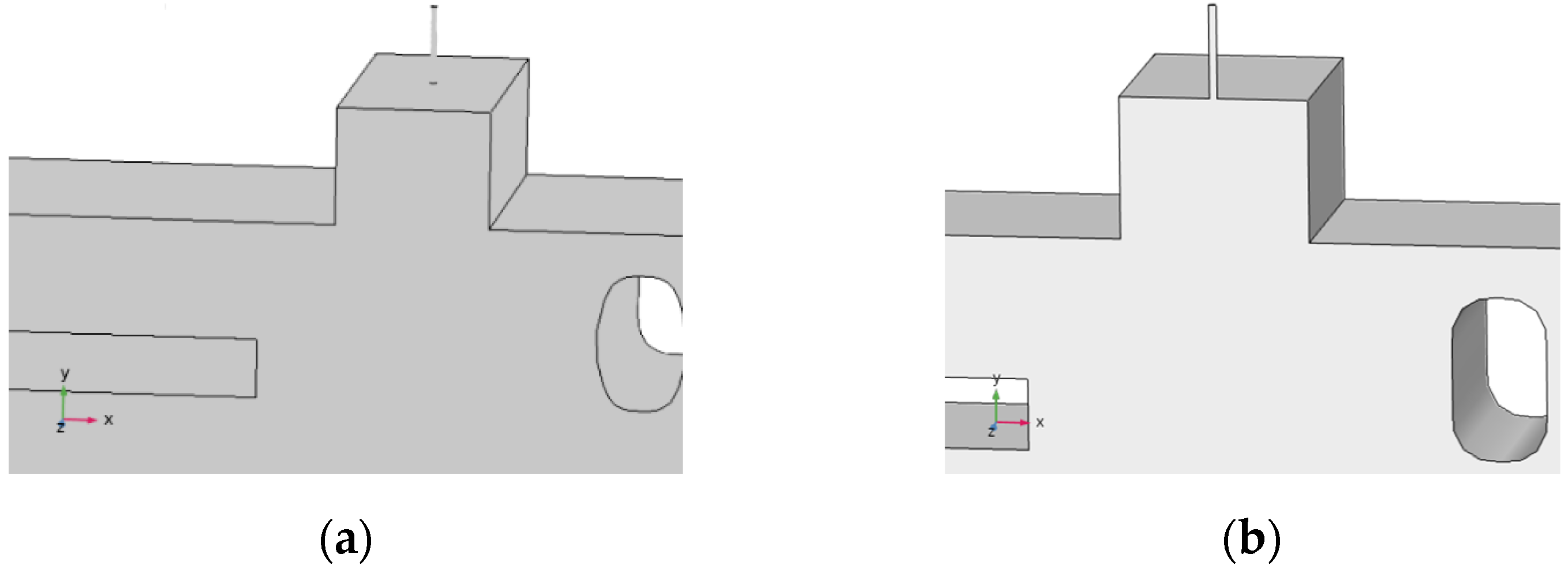
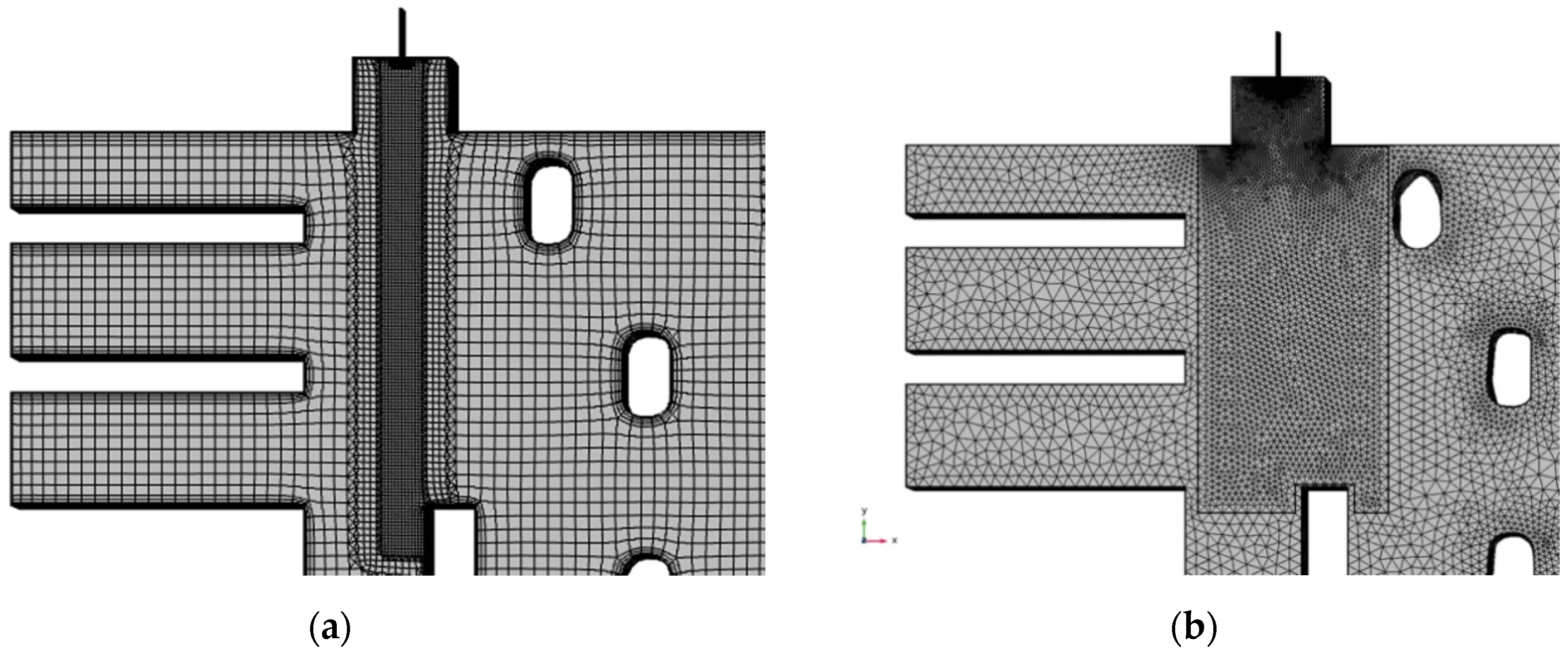
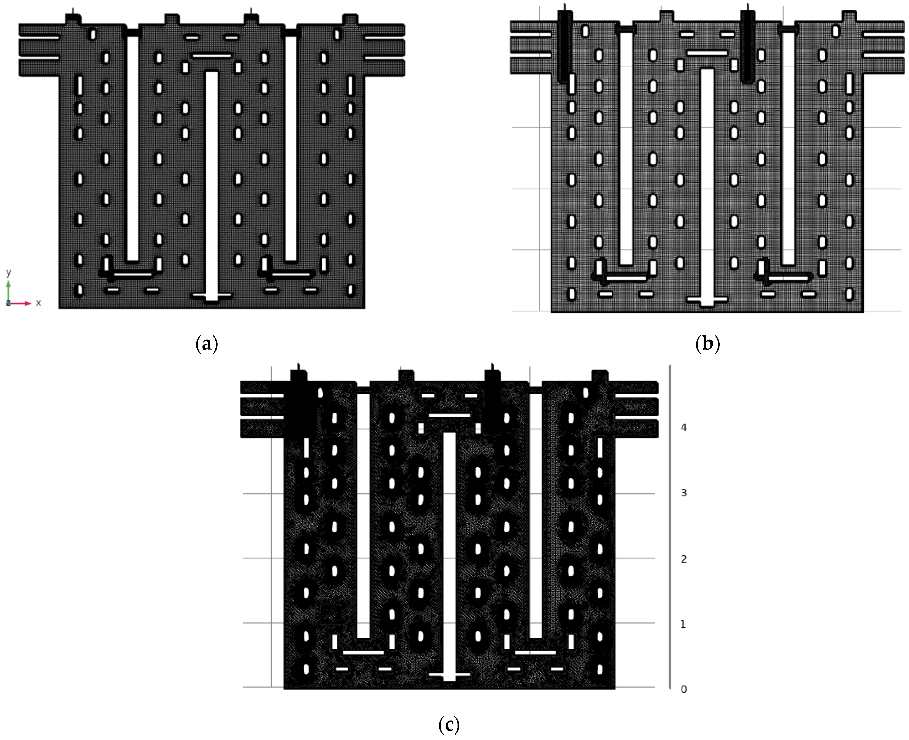
4.1. Geometry and Mesh
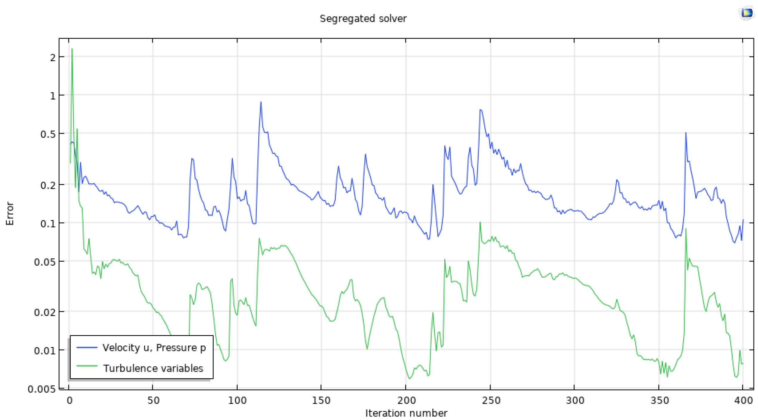
4.2. Simulations
4.3. Numerical Implementation
4.3.1. Finite Element Method in CFD
- It is a very general method,
- There is more facility to increment the element order,
- Physical fields may be reproduced more accurately,
- Physics and mathematics often require different type of functions for a phenomenon. Different phenomena can be represented at the same time with FEM,
- To reach more accuracy, increase order of polynomials and refine the mesh.
4.3.2. Theoretical Definition of FEM
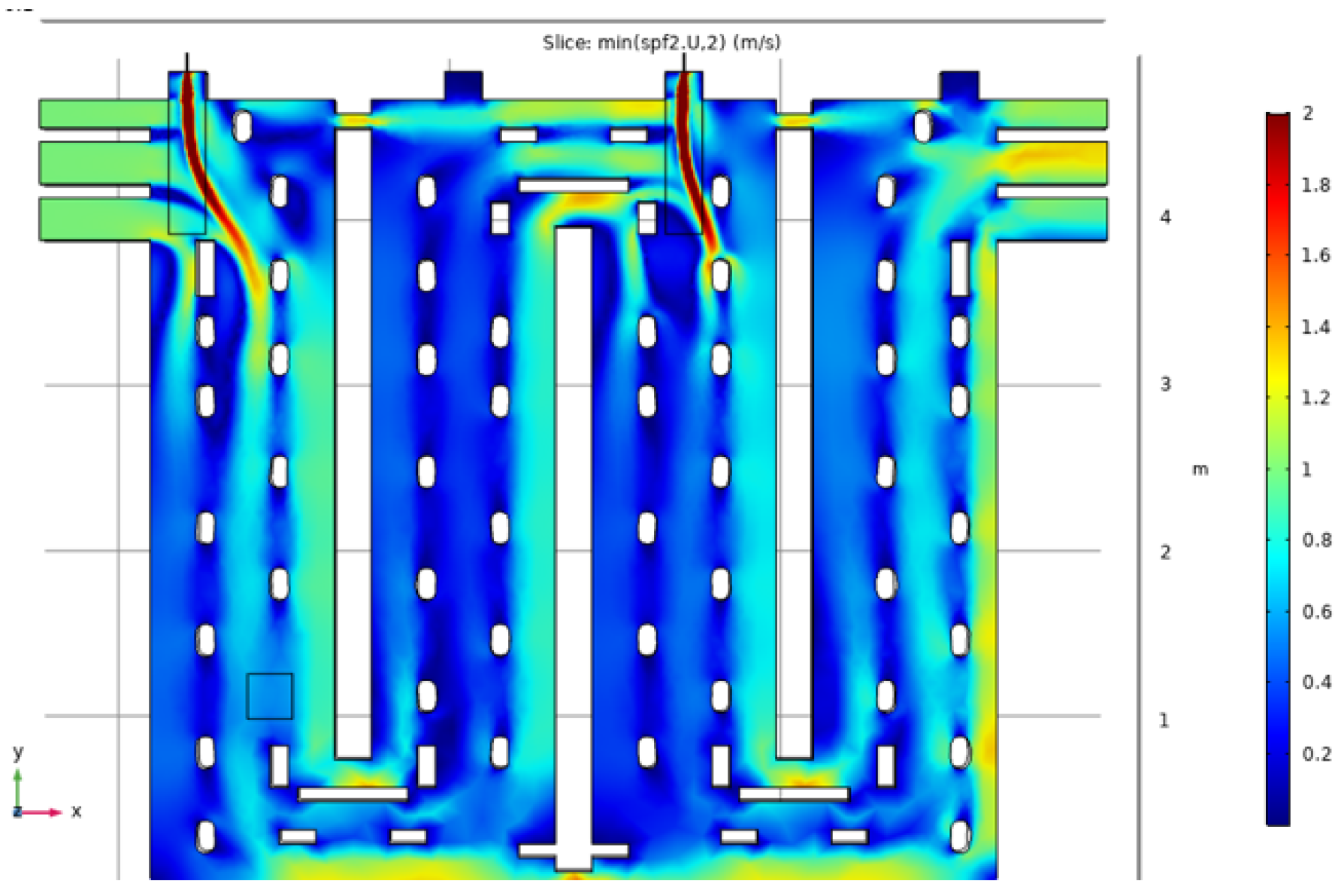
5. Results and Discussion
6. Conclusions
Author Contributions
Funding
Data Availability Statement
Acknowledgments
Conflicts of Interest
Appendix A. Test Using a Fourth Mesh


Appendix B. Wall Resolution from Different Isotropic Diffusion δ Parameters

References
- Severo, D.S.; Gusberti, V. User-friendly software for simulation of anode baking furnaces. In Proceedings of the 10th Australasian Aluminum Smelting Technology Conference, Launceston, Australia, 9–14 October 2011. [Google Scholar]
- Mahieu, P.; Sedmak, P. Improving fuel gas injection in anode baking furnace. In Light Metals 2014; Springer: Berlin/Heidelberg, Germany, 2014; pp. 1165–1169. [Google Scholar]
- Directive, C. Directive 2010/75/EU of the European Parliament and of the Council. Off. J. Eur. Union 2010, 334, 17–119. [Google Scholar]
- Nakate, P.; Lahaye, D.; Vuik, C.; Talice, M. Analysis of the aerodynamics in the heating section of an anode baking furnace using non-linear finite element simulations. Fluids 2021, 6, 46. [Google Scholar] [CrossRef]
- Nakate, P.; Lahaye, D.; Vuik, C.; Talice, M. Computational Study of the Anode Baking Industrial Furnace; The American Flame Research Committee (AFRC): Lakewood Ranch, FL, USA, 2019. [Google Scholar]
- Nakate, P.; Lahaye, D.; Vuik, C. Numerical Modeling of Anode Baking Furnace with COMSOL Multiphysics®. In Proceedings of the 2018 COMSOL Conference, Lausanne, Switzerland, 22 October 2018. [Google Scholar]
- Talice, M. TU-Delft Technical Report Report 01/2018; Technical Report; PMSQUARED Engineering: Delft, The Netherlands, 2018. [Google Scholar]
- Juretić, F. cfMesh Version 1.1 Users Guide. Available online: http://cfmesh.com/wp-content/uploads/2015217/09/User_Guide-cfMesh_v1.1.pdf (accessed on 1 August 2020).
- COMSOL Multiphysics Version 5.5 Reference Manual. Available online: https://doc.comsol.com/5.5/doc/com.comsol.help.comsol/COMSOL_ReferenceManual.pdf (accessed on 1 August 2020).
- Severo, D.S.; Gusberti, V.; Pinto, E.C. Advanced 3D modelling for anode baking furnaces. Light Metals 2005, 2005, 697–702. [Google Scholar]
- Keller, F.; Mannweiler, U.; Severo, D. Computational Modeling in Anode Baking; R&D Carbon Ltd.: Sierre, Switzerland, 2006; pp. 1–12. [Google Scholar]
- Goede, F. Refurbishment and modernization of existing anode baking furnace. Light Metals 2007, 1984, 973–976. [Google Scholar]
- Bui, R.; Dernedde, E.; Charette, A.; Bourgeois, T. Mathematical simulation of a horizontal flue ring furnace. In Essential Readings in Light Metals; Springer: Berlin/Heidelberg, Germany, 2016; pp. 386–389. [Google Scholar]
- Kocaefe, Y.; Dernedde, E.; Kocaefe, D.; Ouellet, R.; Jiao, Q.; Crowell, W. A 3D Mathematical Model for the Horizontal Anode Baking Furnace; Technical Report; Minerals, Metals and Materials Society: Warrendale, PA, USA, 1996. [Google Scholar]
- Severo, D.S.; Gusberti, V.; Sulger, P.O.; Keller, F.; Meier, M.W. Recent developments in anode baking furnace design. In Light Metals 2011; Springer: Berlin/Heidelberg, Germany, 2011; pp. 853–858. [Google Scholar]
- Zhou, P.; Mei, C.; Zhou, J.M.; Zhou, N.J.; Xu, Q.H. Simulation of the influence of the baffle on flowing field in the anode baking ring furnace. J. Cent. South Univ. Technol. 2002, 9, 208–211. [Google Scholar] [CrossRef]
- Ordronneau, F.; Gendre, M.; Pomerleau, L.; Backhouse, N.; Berkovich, A.; Huang, X. Meeting the challenge of increasing anode baking furnace productivity. In Light Metals 2011; Springer: Berlin/Heidelberg, Germany, 2011; pp. 865–870. [Google Scholar]
- Baiteche, M.; Kocaefe, D.; Kocaefe, Y.; Marceau, D.; Morais, B.; Lafrance, J. Description and applications of a 3D mathematical model for horizontal anode baking furnaces. In Light Metals 2015; Springer: Berlin/Heidelberg, Germany, 2015; pp. 1115–1120. [Google Scholar]
- Zaidani, M.; Al-Rub, R.A.; Tajik, A.R.; Shamim, T. 3D Multiphysics model of the effect of flue-wall deformation on the anode baking homogeneity in horizontal flue carbon furnace. Energy Procedia 2017, 142, 3982–3989. [Google Scholar] [CrossRef]
- Kocaefe, Y.; Oumarou, N.; Baiteche, M.; Kocaefe, D.; Morais, B.; Gagnon, M. Use of mathematical modelling to study the behavior of a horizontal anode baking furnace. In Light Metals 2013; Springer: Berlin/Heidelberg, Germany, 2016; pp. 1139–1144. [Google Scholar]
- Valen-Sendstad, K.; Mortensen, M.; Langtangen, H.P.; Reif, B.; Mardal, K.A. Implementing a k-Epsilon Turbulence Model in the FEniCS Finite Element Programming Environment. In Proceedings of the Fifth National Conference on Computational Mechanics, Trondheim, Norway, 26–27 May 2009. [Google Scholar]
- Oumarou, N.; Kocaefe, D.; Kocaefe, Y.; Morais, B. Transient process model of open anode baking furnace. Appl. Therm. Eng. 2016, 107, 1253–1260. [Google Scholar] [CrossRef]
- Oumarou, N.; Kocaefe, D.; Kocaefe, Y. An advanced dynamic process model for industrial horizontal anode baking furnace. Appl. Math. Model. 2018, 53, 384–399. [Google Scholar] [CrossRef]
- Oumarou, N.; Kocaefe, Y.; Kocaefe, D.; Morais, B.; Lafrance, J. A dynamic process model for predicting the performance of horizontal anode baking furnaces. In Light Metals 2015; Springer: Berlin/Heidelberg, Germany, 2015; pp. 1081–1086. [Google Scholar]
- Tajik, A.R.; Shamim, T.; Al-Rub, R.K.A.; Zaidani, M. Performance analysis of a horizontal anode baking furnace for aluminum production. In Proceedings of the ICTEA, International Conference on Thermal Engineering, Muscat, Oman, 26–28 February 2017; Volume 2017. [Google Scholar]
- Tajik, A.R.; Shamim, T.; Al-Rub, R.K.A.; Zaidani, M. Two dimensional CFD simulations of a flue-wall in the anode baking furnace for aluminum production. Energy Procedia 2017, 105, 5134–5139. [Google Scholar] [CrossRef]
- Tajik, A.R.; Shamim, T.; Zaidani, M.; Al-Rub, R.K.A. The effects of flue-wall design modifications on combustion and flow characteristics of an aluminum anode baking furnace-CFD modeling. Appl. Energy 2018, 230, 207–219. [Google Scholar] [CrossRef]
- Chaodong, L.; Yinhe, C.; Shanhong, Z.; Haifei, X.; Yi, S. Research and application for large scale, high efficiency and energy saving baking furnace technology. In TMS Annual Meeting & Exhibition; Springer: Berlin/Heidelberg, Germany, 2018; pp. 1419–1423. [Google Scholar]
- El Ghaoui, Y.; Besson, S.; Drouet, Y.; Morales, F.; Tomsett, A.; Gendre, M.; Anderson, N.M.; Eich, B. Anode baking furnace fluewall design evolution: A return of experience of latest baffleless technology implementation. In Light Metals 2016; Springer: Berlin/Heidelberg, Germany, 2016; pp. 941–945. [Google Scholar]
- Talice, M. TU-Delft Technical Report Report 01/2019; Technical Report; PMSQUARED Engineering: Delft, The Netherlands, 2019. [Google Scholar]
- Gregoire, F.; Gosselin, L.; Alamdari, H. Sensitivity of carbon anode baking model outputs to kinetic parameters describing pitch pyrolysis. Ind. Eng. Chem. Res. 2013, 52, 4465–4474. [Google Scholar] [CrossRef]
- Grégoire, F.; Gosselin, L. Comparison of three combustion models for simulating anode baking furnaces. Int. J. Therm. Sci. 2018, 129, 532–544. [Google Scholar] [CrossRef]
- Wilcox, D. Turbulence Modeling for CFD, 2nd ed.; DCW Industries: La Canada Flintridge, CA, USA, 1998; Volume 2. [Google Scholar]
- Quarteroni, A.; Quarteroni, S. Numerical Models for Differential Problems; Springer: Berlin/Heidelberg, Germany, 2009; Volume 2. [Google Scholar]
- Krizek, M.; Neittaanmaki, P.; Stenberg, R. Finite Element Methods: Fifty Years of the Courant Element; CRC Press: London, UK, 2016. [Google Scholar]
- Donea, J.; Huerta, A. Finite Element Methods for Flow Problems; John Wiley & Sons: New York, NY, USA, 2003. [Google Scholar]
- Ferziger, J.H.; Perić, M.; Street, R.L. Computational Methods for Fluid Dynamics; Springer: Berlin/Heidelberg, Germany, 2002; Volume 3. [Google Scholar]
- Wegner, J.; Ganzer, L. Numerical simulation of oil recovery by polymer injection using COMSOL. In Proceedings of the Excerpt from the Proceedings of the 2012 COMSOL Conference, Milan, Italy, 10–12 October 2012. [Google Scholar]
- Understanding Stabilization Methods. Available online: https://www.comsol.com/blogs/understanding-stabilization-methods/ (accessed on 1 August 2020).


| Authors | Year | Objectives | Combustion Model | Detailed Kinetics | Radiation Model |
|---|---|---|---|---|---|
| Ping. et al. | 2002 | Influence of the baffles on the flowing field | Non-reactive flow | Not included | Not included |
| Severo et al. | 2005 | Developing a 3D CFD model for flue-wall design modification | EDM | Not included | P1 |
| Ordronneau et al. | 2006 | Application of CFD simulation for crossover design off-gas cleaning system optimisation training purposes | Not specified | Not specified | Not specified |
| Gregoire et al. | 2011 | Comparison of two modelling approaches to predict variability | Hot air jet approximation | Not specified | DO method |
| Kocaefe et al. | 2013 | Different modelling approaches on anode baking furnace | Not mentioned | Not included | Not specified |
| Baiteche et al. | 2015 | Effects of flue-wall deformation and employing different radiation models | Empirical kinetic expression | Not included | - P1 - Monte Carlo method |
| Ghaui et al. | 2016 | Implementation of baffleless flue-wall technology | Not mentioned | Not included | Not specified |
| Zaidani et al. | 2017 | Effects of flue-wall deformation | Non-reactive flow | Not included | Not specified |
| Chaodong et al. | 2018 | Optimisation and development of the furnace structures, process parameters and firing control system | Not specified | Not specified | Not specified |
| Nakate et al. | 2018 | Develop a mathematical 2D model to reduce NOx emissions considering turbulent flow, combustion model and radiation | EDM | - κ–ε - Spalart Allmaras | - P1 - DO |
| Talice | 2018 | Develop a 2D model to analyse flow behaviour | Not used | Spalart Allmaras | Not used |
| Nakate et al. | 2019 | Develop a 3D model to analyse flow behaviour | Not used | κ–ε | Not used |
| Talice | 2019 | Develop a 3D model to analyse flow behaviour | Not used | κ–ε | Not used |
| Nakate et al. | 2021 | Establish an analysis in 3D flow with a high rate of fuel injection | Energy equation | - Standard κ–ε - Realizable κ–ε | Not used |
| Parameter | Model 1 | Model 2 | Model 3 | Model 4 | Model 5 | Model 6 | Model 7 | Model 8 | Model 9 |
| Fluid properties | |||||||||
| Density (k/m3) | 1.2 | 1.2 | 1.2 | 1.2 | 1.2 | 1.2 | 1.2 | 1.2 | 1.2 |
| Dynamic viscosity (Pa·s) | 8.9 × 10⁻⁴ | 1.8 × 10⁻⁵ | 8.9 × 10⁻⁴ | 1.8 × 10⁻⁵ | 1.8 × 10⁻⁵ | 1.8 × 10⁻⁵ | 1.8 × 10⁻⁵ | 1.8 × 10⁻⁵ | 1.8 × 10⁻⁵ |
| Initial values for Newton’s iteration | |||||||||
| Ux (m/s) | 70 | 0 | 70 | 0 | 0 | 0 | 0 | 0 | 0 |
| Uy (m/s) | 0 | 0 | 0 | 0 | 0 | 0 | 0 | 0 | 0 |
| Uz (m/s) | 0 | 0 | 0 | 0 | 0 | 0 | 0 | 0 | 0 |
| Pressure (Pa) | 0 | 0 | 0 | 0 | 0 | 0 | 0 | 0 | 0 |
| Boundary conditions | |||||||||
| Wall | No slip | ||||||||
| Inlet | Fully developed flow | ||||||||
| Outlet | Pressure | ||||||||
| Geometry and mesh | |||||||||
| Geometry | 1 | 1 | 1 | 1 | 2 | 2 | 2 | 2 | 2 |
| Mesh | 1 | 1 | 1 | 1 | 2 | 2 | 3 | 3 | 2 |
| Mesh generator tool | cfM | cfM | cfM | cfM | cfM | cfM | COMS | COMS | cfM |
| Artificial diffusion scheme | |||||||||
| δ(u,p) | Off | Off | Off | Off | Off | 0.005 | 0.25 | Off | Off |
| δ(κ,ε) | Off | Off | Off | Off | Off | Off | 0.25 | Off | Off |
| Results used as initial value for the Newton Raphson method | |||||||||
| Initial value | 0 | 0 | 0 | 0 | 0 | δ(u,p) = 0.01 | 0 | Model 7 | Model 8 |
| Mesh | Mesh 1 | Mesh 2 | Mesh 3 |
|---|---|---|---|
| Generator | cfMesh | cfMesh | COMSOL |
| Symmetry | No | Yes | Yes |
| Length x-axis (m) | 5.5 | 5.5 | 5.5 |
| Length y-axis (m) | 5.0 | 5.0 | 5.0 |
| Length z-axis (m) | 0.54 | 0.27 | 0.27 |
| Location of fuel inlet pipes (z-axis) (m) | 0.27 | 0.27 | 0.27 |
| Cell shape | Cartesian | Cartesian | Tetrahedral |
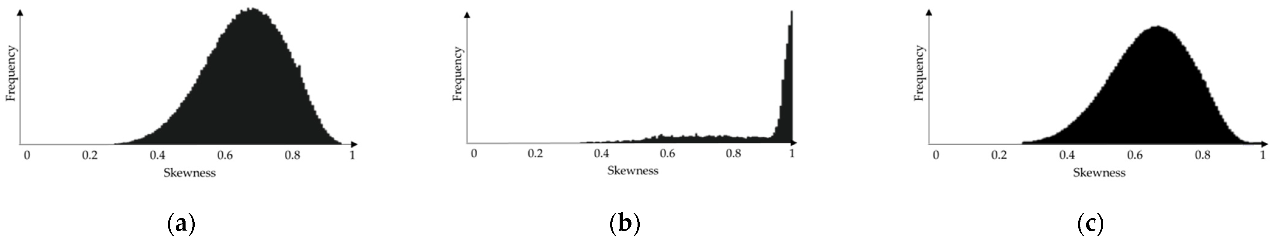
| Mesh | Number of Cells | Minimum Skewness | Average Skewness |
|---|---|---|---|
| Mesh 1 | 2,424,973 | 0.00 | 0.79 |
| Mesh 2 | 545,694 | 0.23 | 0.86 |
| Mesh 3 | 4,924,080 | 0.08 | 0.66 |
| Model | Model 1 | Model 2 | Model 3 | Model 4 | Model 5 | Model 6 | Model 7 | Model 8 | Model 9 |
|---|---|---|---|---|---|---|---|---|---|
| Lowest error reached (u,p) | 10−3 | 10−3 | 10−3 | 10−2 | 10−1 | 10−3 | 10−3 | 10−3 | 10−2 |
| Lowest error reached (κ,ε) | 10−3 | 10−3 | 10−3 | 10−2 | 10−3 | 10−3 | 10−3 | 10−3 | 10−2 |
Publisher’s Note: MDPI stays neutral with regard to jurisdictional claims in published maps and institutional affiliations. |
© 2021 by the authors. Licensee MDPI, Basel, Switzerland. This article is an open access article distributed under the terms and conditions of the Creative Commons Attribution (CC BY) license (https://creativecommons.org/licenses/by/4.0/).
Share and Cite
Libreros, J.; Trujillo, M. Effects of Mesh Generation on Modelling Aluminium Anode Baking Furnaces. Fluids 2021, 6, 140. https://doi.org/10.3390/fluids6040140
Libreros J, Trujillo M. Effects of Mesh Generation on Modelling Aluminium Anode Baking Furnaces. Fluids. 2021; 6(4):140. https://doi.org/10.3390/fluids6040140
Chicago/Turabian StyleLibreros, Jose, and Maria Trujillo. 2021. "Effects of Mesh Generation on Modelling Aluminium Anode Baking Furnaces" Fluids 6, no. 4: 140. https://doi.org/10.3390/fluids6040140
APA StyleLibreros, J., & Trujillo, M. (2021). Effects of Mesh Generation on Modelling Aluminium Anode Baking Furnaces. Fluids, 6(4), 140. https://doi.org/10.3390/fluids6040140