Article

Micropolar Blood Flow in a Magnetic Field

by
George C. Bourantas
School of Engineering, Mechanical Engineering, The University of Western Australia, 35 Stirling Highway, Perth 6009, WA, Australia
Fluids 2021, 6(3), 133; https://doi.org/10.3390/fluids6030133
Submission received: 12 February 2021 / Revised: 8 March 2021 / Accepted: 19 March 2021 / Published: 23 March 2021
(This article belongs to the Special Issue Fluids in Magnetic/Electric Fields)

Abstract

:
In this paper we numerically solve a flow model for the micropolar biomagnetic flow (blood flow) in a magnetic field. In the proposed model we account for both electrical and magnetic properties of the biofluid and we investigate the role of microrotation on the flow regime. The flow domain is in a channel with an unsymmetrical single stenosis, and in a channel with irregular multi-stenoses. The mathematical flow model consists of the Navier–Stokes (N–S) equations expressed in their velocity–vorticity (uω) variables including the energy and microrotation transport equation. The governing equations are solved by using the strong form meshless point collocation method. We compute the spatial derivatives of the unknown field functions using the discretization correction particle strength exchange (DC PSE) method. We demonstrate the accuracy of the proposed scheme by comparing the numerical results obtained with those computed using the finite element method.

1. Introduction

Numerical simulation of biological fluids in the presence of magnetic fields (biomagnetic fluid dynamics (BFD)) has attracted considerable attention over the last decades. Numerous research studies have been published, mainly related to bioengineering (e.g., development of magnetic devices for cell separation, development of magnetic tracers) and medical applications (e.g., targeted transport of drugs using magnetic particles as drug carriers) [1,2]. The majority of biological fluids are considered as biomagnetic, mainly because they contain ions which interact with the applied magnetic field. Blood in particular, has erythrocytes that have the tendency to orient with their disk plane parallel to the magnetic field direction [3], and behaves as a diamagnetic material when oxygenated and as a paramagnetic material when deoxygenated [4].
The first mathematical model that described BFD flow under the action of an applied magnetic field was developed by Haik et al. [1]. In Haik’s model, biofluids were modelled as isothermal, electrically non-conducting magnetic fluids (ferrofluids). Blood was modelled as a magnetic fluid, with its erythrocytes (due to erythrocytes blood exhibits polarization) being magnetic dipoles and the plasma the liquid carrier. Additionally, the ions in the blood plasma interact with an applied magnetic field. Therefore, blood can be modelled as an electrically conducting fluid which exhibits magnetization, such that magnetohydrodynamics (MHD) [5] could also be incorporated into the mathematical model.
In theoretical hydrodynamics the study of a fluid with inner microstructure is considered as an interesting and challenging topic. The concept of microfluids introduced by Eringen [6] to characterize concentrated suspensions of neutrally buoyant deformable particles in a viscous fluid. In micropolar fluids (a subclass of microfluids), rigid particles which are contained in a small representative volume element can rotate about the center of the volume, and their motion is by the microrotation vector [7,8]. The local rotation of the particles is independent of the mean fluid flow and the local vorticity flow field [8]. Micropolar flow theory describes the non-Newtonian behavior of a category of fluids, such as liquid crystals, ferro-liquids, colloidal fluids, liquids with polymer additives, animal blood carrying deformable particles (platelets), clouds with smoke, suspensions, liquid crystals [8,9]. Additionally, micropolar fluids exhibit micro-rotational and micro-inertial effects. Therefore, the main advantage of using a micropolar fluid model to study the blood flow over non-Newtonian fluid models is that micropolar models incorporates the rotation of the fluid particles by means of an independent kinematic vector called the microrotation vector.
Fluid flow is different in micro scale compared to macro scale. In fact, there are flows where the Navier–Stokes equations, as derived through classical continuum theory, become incapable of explaining the micro scale fluid transport phenomena [10]. Micropolar theories, which account for the microstructure of the fluid, appear as an alternative approach to numerically solve micro scale fluid dynamics, which are more computationally efficient than molecular dynamics (MD) simulations. Apart from the theoretical studies on micropolar fluid flow, there are studies that use micropolar theories to explain experimental observations in microchannels [11,12,13,14]. These experiments demonstrated the difference in flow regime of microflows and highlighted that in microscale fluid flows several effects, which are typically excluded from the macroscale (e.g., micro-rotational effects due to rotation of molecules), become important.
There are many physiological fluids that behave like suspensions of deformable or rigid particles in a Newtonian fluid. For example, blood is a suspension of red cells, white cells and platelets in plasma. Blood is a fluid that can be modelled as a micropolar fluids [6,9]. The experimental study of Bugliarello and Sevilla [15] showed that blood plasma can be modelled like a Newtonian fluid and the erythrocytes like a Non-Newtonian core fluid region. Several theoretical studies [16,17,18] on blood flow have assumed that blood behaves either as a Newtonian or as a non-Newtonian fluid. However, these studies fail to provide an estimate of the motion of red cells, white cells and platelets in plasma. It is therefore crucial to study the rheological properties of red and white cells and platelets to determine blood flow resistance in arteries and in vessels. Blood is a typical biomagnetic fluid due to the interaction of intercellular protein, cell membrane and hemoglobin.
In this study, we consider the biomagnetic fluid flow (blood flow), under the action of a magnetic field, for a two-dimensional duct with constriction. The micropolar/biofluid is considered to be viscous, incompressible and Newtonian, with the flow being laminar. The flow is subjected to an external magnetic field, which is generated with a magnet placed at a point in the proximity of the lower plate. The fluid is assumed to be poor conductor so that the induced magnetic field inside the fluid can be neglected. Under this assumption the flow is affected only by the magnetization of the fluid. The momentum equation takes into account the magnetization of the fluid, since the biomagnetic fluid flow is affected by the magnetization of the fluid due to the presence of the magnetic field. Although the fluid exhibits electrical conductivity, it may be taken as a poor conductor in which Lorentz force arising in magneto-hydrodynamics is much smaller in comparison to the magnetization force. Finally, it is also assumed that the magnetization of the biomagnetic fluid is varying linearly with the temperature of the fluid and the strength of the magnetic field.
We numerically solve the governing equations using the well-established meshless point collocation (MPC) method. The MPC method has been successfully applied to numerous problem in science and engineering involving fluid and solid mechanics applications, such as elasticity [19], crack propagation [20], heat transfer [21], flow in porous media [22], transport phenomena, to name a few. In particular, the proposed meshless scheme has been applied to a number of biomedical applications, such as tumor ablation [23], neurosurgery [24], soft tissue deformation [25] and electrophysiology [26]. This paper is organized as follows: in Section 2 we present the governing equations, while in Section 3 we briefly describe the discretization correction particle strength exchange (DC PSE) differentiation method and we discuss the solution procedure. issues related to the accuracy and the computational cost of the proposed scheme. In Section 4 we verify the accuracy of our algorithm by comparing our results to finite element solutions. In Section 5 we demonstrate the accuracy, efficiency and the ease of use of the proposed scheme using numerical examples. Finally, Section 6 contains discussion and conclusions.

2. Governing Equations

We consider the laminar incompressible flow of a homogeneous, micropolar, Newtonian and electrically conducting fluid (blood). The micropolar fluid flows under the influence of a magnetic field. Two major forces act on the fluid, magnetization and Lorenz force. The first, applies due to the orientation of the erythrocytes along the magnetic field, while the second arises due to the electric current generating from the moving ions in the plasma. The biofluid under investigation (blood) is subjected to equilibrium magnetization, and its apparent viscosity due to magnetic field is negligible. Additionally, the contribution of the Lorentz force is incorporated in the mathematical model adopting flow principles of magnetohydrodynamics (MHD).
The following assumptions are made regarding of the blood flow: blood is an electrically conducting biomagnetic Newtonian fluid [27,28,29]; the flow is laminar and the viscosity due to the magnetic field is considered to be negligible; the rotational forces acting on the erythrocytes when they enter and exit the magnetic field are discarded (equilibrium magnetization); the walls of the channel are electrically nonconducting and the electric field is considered negligible. Under these assumptions the governing flow equations are extended as:
ρ f * u * t + u * · u * = p * + μ f + κ ν 2 u * + κ ν × N * + μ 0 * M * H * + J ×
· u * = 0
ρ f * j N * t + u * · N * = γ ν 2 N * + κ ν × u * 2 κ ν N *
ρ f * C p T t + u * · T + μ 0 * T M * T D H * D t J · J σ f * = α f 2 T + μ f Φ
where u * is the velocity vector, p * is the pressure, T* is the fluid temperature and N* is the microrotation vector, J = σ f * u * × B   is the density of the electric current, B is the magnetic induction, σ f * is the electrical conductivity of the fluid, D / D t = / t + u * · is the Stokes tensor, M *   is the magnetization, H * is the magnetic field intensity. Additionally, we assume that fluid mass density ρ f * , dynamic viscosity μ f , specific isobaric heat per unit mass C p , heat conduction α f and all micropolar fluid properties such as vortex viscosity coefficient κ ν and microinertia j , are constant parameters. Φ is the dissipation function which for the three-dimensional case has the form (dropping the terms for the z- component of velocity, and spatial derivatives with respect of z we obtain the expression in two dimensions):
Φ = 2 u x 2 + v y 2 + w z 2 + v x + u y 2 + w y + v z 2 + u z + w x 2 2 3 u x + v y + w z 2
We consider flow in two dimensions and we write the governing equations in their velocity–vorticity formulation. We solve the steady-state N–S equations and therefore we drop the transient terms form the governing equations. For the case of two-dimensional plane flow the governing equations, in the velocity–vorticity formulation, are written as:
2 u * = ω * y *
2 v * = ω * x *
ρ f * u * ω * x * + v * ω * y * = μ f + κ ν 2 ω * κ ν 2 N * + μ 0 * M * x * H * y * M * y * H * x * σ f * B 2 u * y *
ρ f * j u * N * x * + v * N * y * = γ f 2 N * 2 κ ν N * + κ ν ω *
ρ f * C p u * T * x * + v * T * y * + μ 0 T M * T u * H * x * + v * H * y * σ f * B 2   u * 2 = α f 2 T + μ f 2 u * x * 2 + 2 v * y * 2 + v * x * + u * y * 2
The term μ 0 T M * T u * H * x * + v * H * y * represents the thermal power per unit volume due to the magnetocaloric effect. The term σ f * B 2   u * 2 in Equation (8) represents the Lorentz force per unit volume and arises due to the electrical conductivity of the fluid, where the same term in Equation (10) represents the Joule heating. The magnetization M * is a function of the magnetic field intensity H * and temperature T , following the formula M * = K M H * T c T derived experimentally in [11], with K M is a constant and T c is the Curie temperature. The components H x * and H y * of the magnetic field intensity H * are given as
H x * = γ 2 π y * b * x * a * 2 + y * b * 2
H y * = γ 2 π x * a * x * a * 2 + y * b * 2
where a * , b * is the location (point) where the magnetic wire (current-carrying conductor) is placed, and γ is the magnetic field strength at this point x = a * , y = b * . The magnitude H *   of the magnetic field intensity is given by:
H * = H x * 2 + H y * 2 1 2 = γ 2 π 1 x * a * 2 + y * b * 2
We use the following non-dimensional parameters:
x = x * D ,   y = y * D ,   u = u * u m ,   v = v * u m ,   H = H * H 0 , ω = ω * D u m ,   N = N * D u m ,   T = T * T w * T f * T w *
with u m being the maximum velocity at the inlet of the channel, T f * and T w * the temperature at the upper and lower wall, respectively, and H 0 = H * a * , 0 . The non-dimensional form of the governing equations as:
2 u = ω y
2 v = ω x
u ω x + v ω y = 1 + K 2 ω 2 N M n F R e H T y H x T x H y + M n M y u H 2
u N x + v N y = 1 + K 2 2 N 2 K N + K ω
P r R e u T x + v T y M n F R e E c ε T H u H x + v H y = 2 T + P r E c 4 u x 2 + ω 2
with the non-dimensional parameters defined as R e = D ρ f * u m μ f   (Reynolds number), E c = u m 2 C p T f * T w * (Eckert number), ε = T w * T f * T w * (Temperature number), P r = C p μ f α f (Prandtl number), M n F = μ 0 * H 0 2 K M T f * T w * ρ f * u m 2 (Magnetic number from ferro-hydrodynamics), M n M = μ 0 * 2 H 0 2 D σ f * μ f (Magnetic number from magneto-hydrodynamics). The magnitude H of the magnetic field intensity is given by the relation H x , y = b x a 2 + y b 2 . The boundary conditions defined as
upper   wall :   u = v = T = N = 0 lower   wall :   u = v = T = N = 0 inlet :   u = 4 y 4 y 2 ,   v = 0 ,   T = 4 y 1 y ,   N x = 0 o u t l e t :   u x = 0 ,   v = 0 ,   T x = N x = 0
For the velocity–vorticity flow equations, we compute the updated vorticity values [30] using the velocity field values and the strong form meshless discretization-corrected particle strength exchange (DC PSE) operators of the first order spatial derivative (see Equation (29)) as ω = v x u y .

3. Numerical Method

3.1. Discretization-Corrected Particle Strength Exchange

The DC PSE method computes spatial derivatives using a set of nodes distributed (uniformly or randomly) over the spatial domain. It was introduced as a Lagrangian particle-based numerical method [31], using the particle strength exchange (PSE) operators [32,33]. To apply to the numerical solution of partial differential equations (PDEs) using the DC PSE meshless method, Bourantas et al. [34] reimplemented the Lagrangian oriented DC PSE method to work in the Eulerian framework.
The DC PSE operators reduce the discretization error ϵ h x in the PSE operator approximation [32,33]. In DC PSE approximation a kernel function minimizes the difference between the DC PSE discrete operator and the actual derivative. To achieve this, we use the following expression [31,34] for the derivative approximation:
Q h β f x = 1 β β ! Z h β D β f x + a   =   1 a β 1 a a ! ε a β Z h a D a f x + r 0
with
r 0 = 0 β   e v e n 2 e β Z h 0 f x β   o d d  
and the discrete moments defined as:
Z h a = 1 ε d p N x   x x p ε a η β x x p ε
The set of moment conditions becomes:
Z h a = 1 β β ! a   =   β 0 a β < otherwise a m i n a β + r 1
with β being a non-negative integer defined as β = β 1 , β 2 , , β n , where β i , i = 1 , 2 , , n . The partial differential operator D β is expressed as D β = β x 1 β 1 x 2 β 2 x n β n . The kernel η β is chosen as:
η β x , z = γ   =   a m i n β + r 1 a γ x z γ e z 2 = P x , z W z ,   z = x x p ε
with weights
w a γ x = 1 ε α + γ + d p N x   x x p α + γ e x x p ε 2
For the approximated derivative Q h β f x at node x p , the coefficients are computed by solving the linear system of equations Equation (25) for x = x p . Given our choice of kernel function, the DC PSE derivative approximation becomes:
Q h β f x p = 1 ε β x p p N x   f x q f x p p x x p ε x p a T x p e x p x q ε x p 2
where p(x) = [p1(x), p2(x), …, pm(x)], with m being the number of monomials (m = 6 and m = 10 for second order monomials in two and three dimensions, respectively), and   a (x) are the vectors of terms in the monomial basis and their coefficients, respectively. By using the DC PSE method, the spatial derivatives Q β up to second order are given as:
Q 1 , 0 x ,   Q 0 , 1 y
and
Q 1 , 1 2 x y = 2 y x ,   Q 2 , 0 2 x 2 ,   Q 0 , 2 2 y 2

3.2. Solution Procedure

The numerical solution of the governing equations deals with the solution of five governing equations (in 2D) plus one equations needed for the velocity-correction method applied to ensure the mass conservation.
The velocity-correction method is an iterative scheme used to numerically solve fluid flow equations [35,36,37]. First, the Poisson equations for the velocity components (Equations (15) and (16)) are solved to obtain the intermediate velocity u ˜ . The intermediate velocity does not, in general, satisfy the continuity equation, that is · u ˜ 0 . To satisfy the continuity equation, we update the velocity field using a velocity correction δ u , such that the updated velocity u k + 1 is written as u k + 1 = u ˜ + δ u . We assume that the velocity correction is irrotational (but not the flow itself), i.e., then a Helmholtz potential (or correction potential) φ k + 1 is defined as φ k + 1 = δ u . The updated velocity satisfies the continuity equation, i.e., · u k + 1 = 0 , and therefore the correction potential satisfies the Poisson-type equation 2 φ k + 1 = · u ˜ . Once this Helmholtz-Poisson problem is solved, the updated velocity field satisfies the continuity equation.
The steps of the iterative method used are:
  • Set an initial value for the velocity field u k   =   u k , v k , vorticity ω k , temperature T k and microrotation N k .
  • Use the velocity components u k = u k , v k in x- and y- direction to calculate the initial vorticity value ω k = v k x u k y and its spatial derivatives ω k x and ω k y .
  • Solve the Poisson equation (Equation (15)) to compute the x- velocity component u ˜ , and Poisson equation (Equation (16)) to compute the y- velocity component v ˜ .
  • Apply the velocity-correction method. Using the velocity components u ˜ , v ˜ computed in the previous step, update the velocity components u k + 1 = u k + 1 , u k + 1 , which now fulfill the incompressibility constraint · u k + 1 = 0 .
  • Using the updated velocity value u k + 1 , solve Equation (17) to obtain the updated vorticity values ω k + 1 . We solve the linear system L ω ω k + 1 = b ω with L ω = 1 + K 2 u k + 1 x v k + 1 y and b ω = M n F R e H T y H x T x H y + M n M y u H 2 with b ω obtaining values from the previous iteration. The updated vorticity values ω k + 1 are computed using the updated velocity values u k + 1 = u k + 1 , v k + 1 computed in the previous step, and by using the formula for vorticity ω k + 1 = v k x u k y to apply vorticity boundary conditions.
  • Using the updated velocity value u k + 1 , solve Equation (18) to obtain the updated microrotation values N k + 1 . We solve the linear system L N N k + 1 = b N with L N = 1 + K 2 2 u k + 1 x v k + 1 y 2 K and b N = K ω k with b N obtaining values from the previous iteration.
  • Using the updated velocity value u k + 1 , solve Equation (13) to obtain the updated temperature values T k + 1 . We solve the linear system L T T k + 1 = b T with L T = 2 P r R e u k + 1 x P r R e v k + 1 y M n F R e E c H u k + ! H x + v k + 1 H y and b T = M n F R e E c ε H u H x + v H y P r E c 4 u x 2 + ω 2 with b N obtaining values from the previous iteration.
  • Compute the normalized root mean square error L N R M S E = i = 1 N q i t + d t q i t 2 N 2 q m a x t q m i n t for each of the unknown field value q.
  • Update the solution using a relaxation factor q = a r f q k + 1 a r f q k + 1 , with q = ω , T , N . By setting q k = q and repeat steps 2–8 until the convergence criteria are met.

4. Algorithm Verification

We verify the accuracy of the proposed scheme by comparing our numerical findings with those reported in [27,
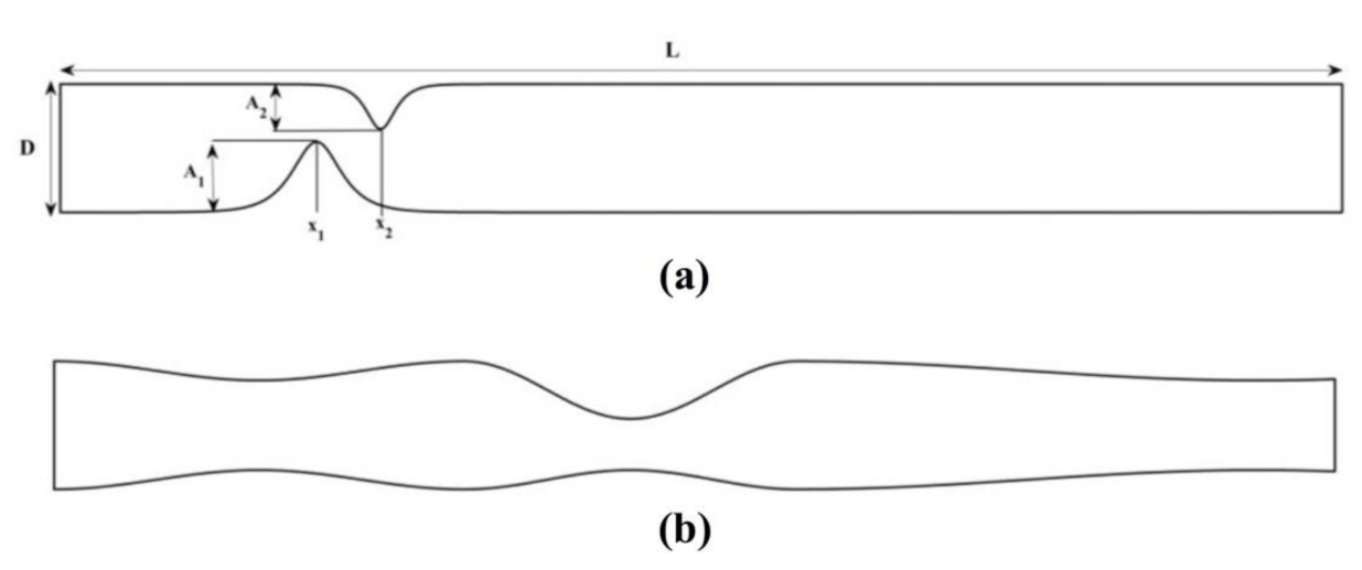
29]. We consider the biomagnetic fluid flow under the influence of an externally applied magnetic field in a channel with an unsymmetrical single stenosis and in a channel with irregular multi-stenoses (Figure 1).
We assign values to the dimensionless parameters described in the governing equations based on the values reported in [27,29]. We set P r = 25 , ε = 77.5 and E c = 1.49 × 10 8 . The length L and the width D of the unconstricted channel are taken as L = 10 and D = 1 , respectively. We use the iterative solution procedure, described in Section 3.2, to obtain a steady-state solution for all the flow cases considered herein. To reach a steady-state solution, we set the convergence tolerance to 10 4 for the vorticity, microrotation and the temperature at each node of the flow domain.

4.1. Unsymmetrical Stenosis

As a first verification example we consider flow in a flow domain with an unsymmetrical stenosis downstream [29] (Figure 1a). The lower and upper walls of the channel are defined as:
y l o w e r = A 1 s e c h B 1 x x 1 ,   0 x 10
y u p p e r = 1 A 2 s e c h B 2 x x 2 ,   0 x 10
The positive constants A1, A2 control the degree of constriction of the channel, while B1, B2 are the constants controlling the length of the stenosed area. The stenosed parts at the lower and the upper plates are positioned at sites with coordinates x1 and x2, respectively. Herein, we considered A1 = 0.5, A2 = 0.4, B1 = 6 and B2 = 4, while the stenosed sites were positioned at x1 = 3 and x2 = 4.
We consider a fixed location of the magnetic source a , b = 3.0 , 0.05 and we use different values for the magnetic numbers M n F and M n M 
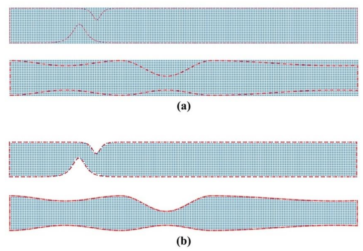
. To represent the flow domain, we use a uniform Cartesian nodal distribution embedded into the flow domain (see Figure 2). The nodal distribution applies by generating a grid that covers the symmetrical stenosis and identifying only those nodes that lie inside the geometry (nodes are also used on the boundaries). We use successively denser computational grids (point clouds) to ascertain a grid independent solution. The coarsest grid (Cloud 1) consists of 56,118 nodes (corresponding to h = 0.0134 node spacing), and the densest (Cloud 4) of 298,176 nodes (corresponding to h = 0.0057 node spacing). Table 1 lists the grid configurations used in the simulations.
To ensure a grid independent numerical solution we project the velocity, vorticity, temperature and stream function values computed using Cloud 1, 2 and 3 into Cloud 4. The results obtained with the finest grid are taken as reference. We apply the projection using the modified moving least s(MMLS) method [38]. The accuracy of the proposed meshless scheme increases with increasing number of nodes and Cloud 3 offers a converged solution (see Table 2).
Table 3 lists the computational time (in seconds) for computing the spatial derivatives for the grid resolutions listed in Table 2, and for the numerical solution of governing equations (for each time iteration) in the case of M n F = 1312 and M n M = 6.4 . It takes roughly 350 iterations to reach a normalized root mean square error of order 10 3 . The efficiency of the proposed scheme appears to be superior to finite element solvers used to numerically solve the steady-state Navier–Stokes equations [39].
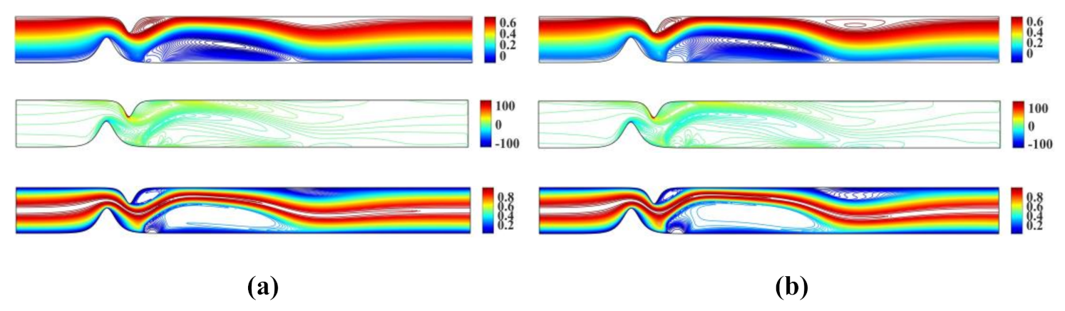
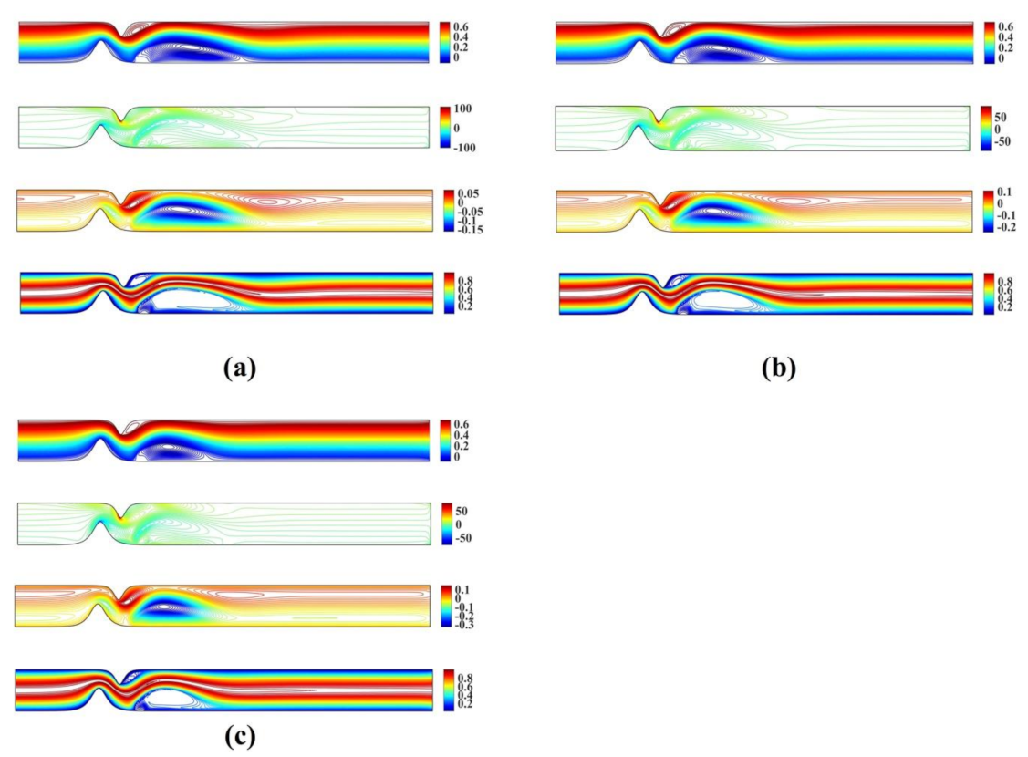
Figure 3 shows the stream function, vorticity and temperature contour plots for M n F = 656 and M n M = 1.2 and M n F = 1312 and M n M = 6.4 , respectively. The numerical results obtained using the proposed meshless scheme are in a very good agreement with the numerical results reported in [27].

4.2. Irregular Multi-Stenoses

In the second verification example, the flow domain is a channel with irregular multi-stenotic regions (see Figure 1b). The flow domain narrows downstream with a symmetric stenosis close to the inlet and recovers its initial width. Then, a severe constriction follows which is unsymmetrically spread in the middle of the channel. After the recovery of the second stenosis, the channel narrows down gradually so that the exit diameter is less than the entrance diameter. The lower and upper walls of the channel are defined as:
y l o w e r = C 1 1 c o s 2 π x D x / E x ,   0 x 10
y u p p e r = 1 C 2 x 1 c o s 2 π x D x E x ,   0 x 10
with C 1 being a positive constant ( C 1 = 0.075 ), and the piecewise constant-valued functions C 2 x , D x and E x defined as:
C 2 x = 0.075 5.8 < x 10 0.225 3.2 < x 5.8 0.075 0 x 3.2 ,
D x = 5.8 5.8 < x 10 3.2 3.2 < x 5.8 0 0 x 3.2
E x = 7.2 5.8 < x 10 2.6 3.2 < x 5.8 3.2 0 x 3.2
To represent the flow domain, we use regular (uniform) nodal distribution embedded into the flow domain. The nodal distribution applies by generating a uniform Cartesian grid that covers the unsymmetrical stenosis and identifying only those nodes that lie inside the geometry (nodes are also used to represent the boundaries). We use a grid that consists of 56,118 nodes (corresponding to h = 0.008 node spacing as in Cloud 3), which offers a converged solution. We consider a fixed location of the magnetic source a , b = 6.0 , 0.05 and we use different values for the magnetic numbers M n F and M n M .
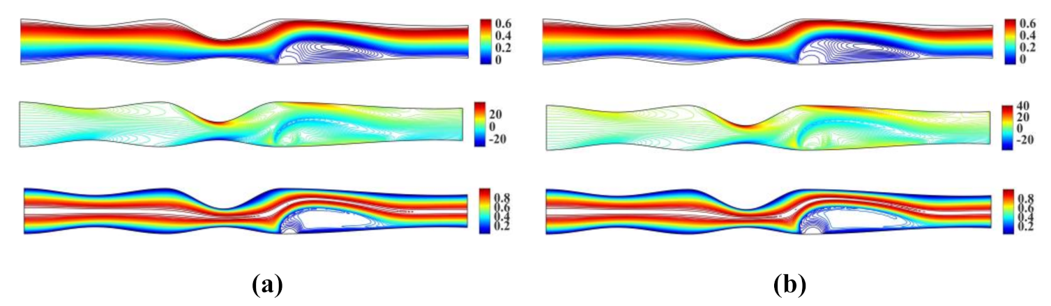
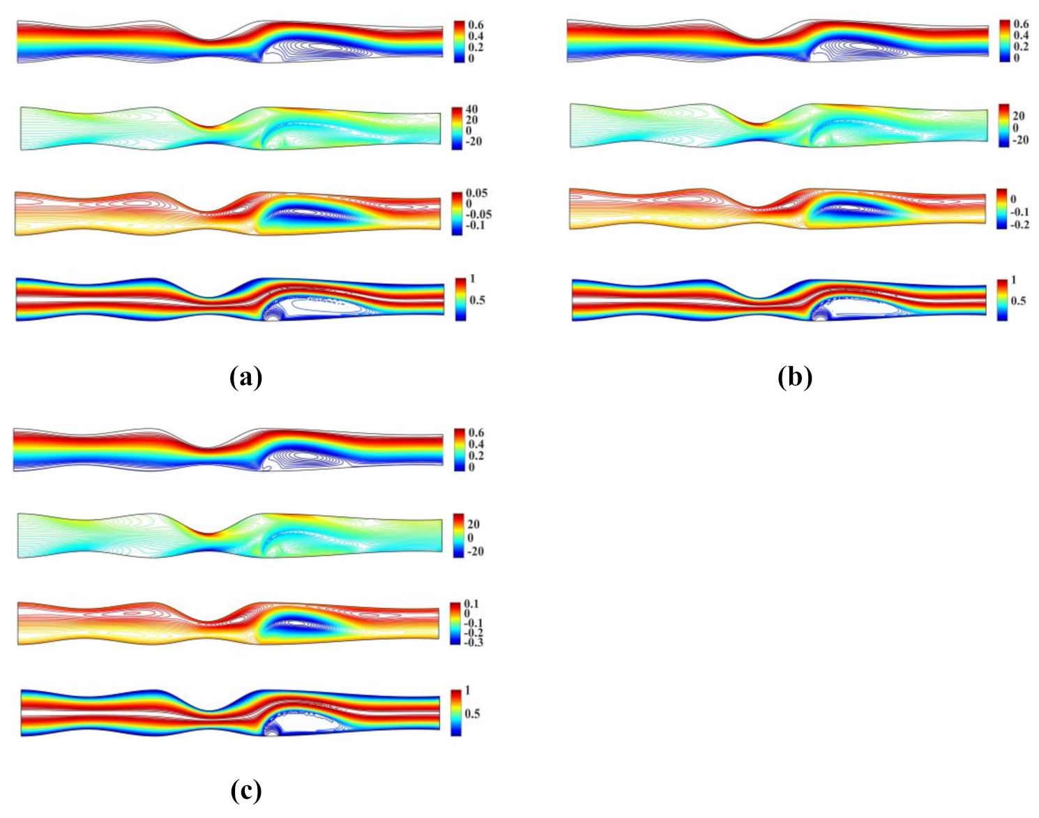
Figure 4 shows the streamlines, vorticity contours and isotherms for M n F = 656 , M n M = 1.2 and M n F = 1312 , M n M = 6.4 , respectively.
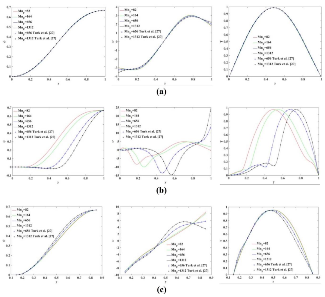
Figure 5 shows the profile plots for the stream function ( ψ ), vorticity ( ω ) and temperature ( T ) at different location of the flow domain, namely at x = 3 ,   6   and 9. The numerical results obtained using the proposed meshless scheme are in a very good agreement with the results presented in [27].

5. Numerical Results

In this section we investigate the influence of microrotation number (K) and Reynolds number R e on the flow regime. The fluid properties, the boundary conditions and external magnetic field, are identical to the previous cases.
We examine the biomagnetic fluid flow under the influence of an externally applied magnetic field in a channel with a single unsymmetrical stenosis, and with irregular multi-stenoses. Numerical studies on Newtonian [11] and non-Newtonian [17] blood flow through stenosed arteries demonstrated that the shape of the stenosis (single or multiple, symmetrical or unsymmetrical) affects the flow regime, and hence deserve special attention.
For the problems considered in this section, we assign flow (dimensionless) parameters directly related to blood flow. The density and dynamics viscosity of the blood are ρ f * = 1050   kg   m 1 and μ f = 3.2 × 10 3   kg   m 1   s 1 , respectively, while the blood flows into the vessel with maximum velocity u m = 1.524 × 10 2   m   s 1 and height (in the unconstricted region) of h = 2.0 × 10 2   m . Furthermore, we consider a magnetic field strength of 8 T, and we set the temperature at the upper and lower wall of the vessel to T u * = 41 °C and T l * = 37 °C. In our study, we consider the Prandtl number P r to be constant, despite that the dynamic viscosity μ f , the specific heat under constant pressure C p and the thermal conductivity α f are temperature dependent. Therefore, for the temperature range considered in this study, we set the specific heat to C p = 3.9 × 10 3   J   kg 1   K 1 and the thermal conductivity to α f = 0.5   J   s 1   K 1 . For the aforementioned values P r = 25 , ε = 77.5 and E c = 1.49 × 10 8 [29]. The length and the width of the unconstricted channel are taken as L = 10 and D = 1 , respectively.

5.1. Dependence on Microrotation Number

In this section, we investigate the influence of the microrotation number (K) on the flow regime (flow dynamics). We consider fluid flow in a channel with a unsymmetrical single stenosis and with irregular multi-stenoses (see Figure 1).
For the unsymmetrical stenosis, we used A1 = 0.5, A2 = 0.4, B1 = 6 and B2 = 4, while the stenosed sites were positioned at x1 = 3 and x2 = 4. We consider a fixed location of the magnetic source a , b = 3.0 , 0.05 . For the multiple stenosis flow case, we used A1 = 0.5, A2 = 0.4, B1 = 6 and B2 = 4, while the lower and the upper plates are positioned at x1 = 3 and x2 = 4, respectively. We consider a fixed location of the magnetic source a , b = 6.0 , 0.05
We use a uniform Cartesian grid, embedded into the irregular geometry, to represent the flow domain. In the unsymmetrical stenosis flow case, a grid of 151,703 nodes (corresponding to h = 0.008 node spacing) is used, while in the channel with multiple stenosis we use a grid of 127,427 nodes (corresponding to h = 0.008 node spacing). Both grid ensure grid independent numerical solutions. In our simulations, we set M n F = 656 , M n M = 1.2 , R e = 100 and K = 0.5 ,   1.0 and 2.0 .
Figure 6 shows the streamlines, vorticity and microrotation contours, along with isotherms for the unsymmetrical stenosis flow case for different Reynolds numbers. It is well observed that the streamlines, vorticity and microrotation contours and the isotherms are distorted from being straight lines in the region after the stenosis. A vortex following the circulation is formed downstream of the stenosis close to the upper wall in both streamlines and isotherm profiles. As the microrotation number increases, the re-attachment length of the vortex decreases (the vortex is actually compressed). Additionally, the vortex formed at the upper wall of the stenosis is also compressed when microrotation number increases. The same pattern appears to vorticity, microrotation and temperature filed values.
Figure 7 shows the streamlines, vorticity and microrotation contours, along with isotherms obtained for the unsymmetrical stenosis flow case. In our simulations, we set M n F = 656 , M n M = 1.2 , R e = 200 and K = 0.5 ,   1.0 and 2.0 .

5.2. Dependence on Reynolds Number

In this section, we investigate the influence of the Reynolds number (Re) on the flow regime. We consider flow in a channel with a unsymmetrical single stenosis, and with irregular multi-stenoses (see Figure 1). For the unsymmetrical stenosis, we used A1 = 0.5, A2 = 0.4, B1 = 6 and B2 = 4, while the stenosed sites were positioned at x1 = 3 and x2 = 4. We consider a fixed location of the magnetic source a , b = 3.0 , 0.05 . For the multiple stenosis flow case, we used A1 = 0.5, A2 = 0.4, B1 = 6 and B2 = 4, while the lower and the upper plates are positioned at x1 = 3 and x2 = 4, respectively. We consider a fixed location of the magnetic source a , b = 6.0 , 0.05 .
We use a uniform Cartesian grid, embedded into the irregular geometry; to represent the flow domain, we use regular (uniform) nodal distribution embedded into the flow domain. In the case of the unsymmetrical stenosis, a grid of 151,703 nodes (corresponding to h = 0.008 node spacing) is used, while in the channel with multiple stenosis we use a grid of 127,427 nodes (corresponding to h = 0.008 node spacing). Both grid ensure grid independent numerical solutions. In our simulations, we set M n F = 656 , M n M = 1.2 , K = 2 and R e = 50 ,   100 ,   200 and 300 .
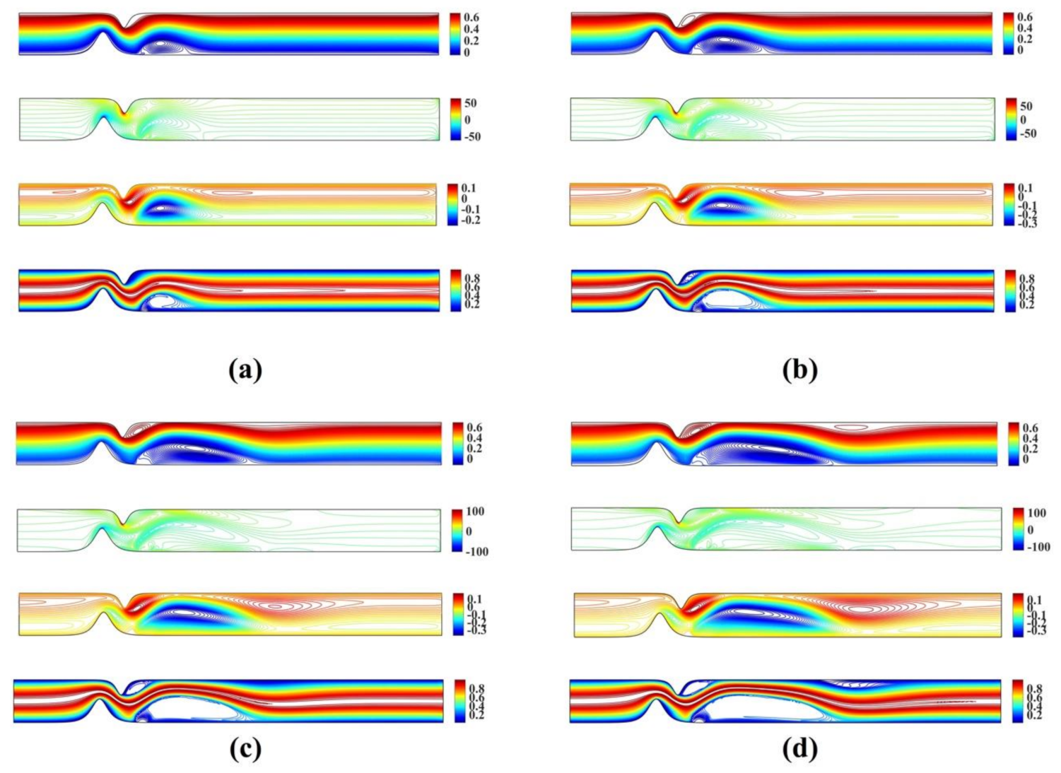
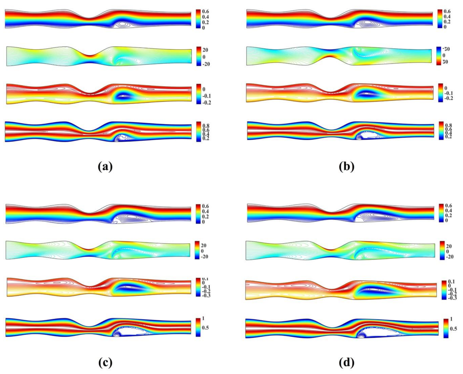
Figure 8 shows the streamlines, vorticity and microrotation contours, and isotherms for the unsymmetrical stenosis flow case for different Reynolds numbers. It is well observed that the streamlines, vorticity contours and the isotherms are distorted from being straight lines in the region after the stenosis. A vortex following the circulation is formed downstream of the stenosis close to the lower wall in both streamlines and isotherm profiles. As Reynolds number increases, a second vortex is formed in the upper wall just after the stenosis. For the microrotation, as the Reynolds number increases the iso-contour lines that form a vortex in the lower wall are stretched downstream and towards the upper wall. Additionally, a secondary vortex appears close to the upper wall.
Figure 9 shows the streamlines, vorticity and microrotation contours, and isotherms for the unsymmetrical stenosis flow case for different Reynolds numbers. It is well observed that the streamlines, vorticity contours and the isotherms are distorted from being straight lines in the region after the stenosis downstream. The vortex which is formed downstream of the stenosis close to the upper wall in both streamlines and isotherm profiles. As the Reynolds number increases, a second vortex is formed in the upper wall just after the stenosis. For the microrotation, as the Reynolds number increases the iso-contour lines that form a vortex in the lower wall are stretched downstream and towards the upper wall. Additionally, a secondary vortex appears close to the upper wall.

6. Conclusions

In this contribution, we extended the magnetohydrodynamics (MHD) model introduced in [28,29] to account for the microrotation of the blood. We utilized a well-established and verified meshless point collocation algorithm to numerically solve the velocity–vorticity formulation of biomagnetic micropolar flow in a magnetic field.
We demonstrate that the proposed scheme works efficiently in complex geometries like the ones shown in Section 4, Algorithm Verification. We highlight the accuracy of the proposed scheme by comparing our numerical results with those computed using the finite element method [27]. An important advantage of our method is the ease and speed with which one can construct computational grids for flow domains with irregular shapes. The meshless scheme based on DC PSE methods to compute spatial derivatives can be used in the case of Cartesian-embedded grids.
We have verified the accuracy of the proposed scheme by comparing our numerical results with those computed using finite element method [27], and the results are in excellent agreement. Our proposed scheme offers several advantages over other commonly used methods:
  • Rapid and easy generation of computational grids, as demonstrated by examples of the flow in a channel with an unsymmetrical stenosis and with multiple stenosis in Section 5.1 and Section 5.2, respectively.
  • High accuracy, as demonstrated in verification examples discussed in Section 4.
  • Easy and straightforward way to impose vorticity boundary conditions using spatial derivatives computed using the DC PSE method (Equation (33)).
  • Simplicity: we use a MATLAB code of ca. 150 lines to solve flow equations, and a C++ code of ca. 140 lines to compute spatial derivatives.

Funding

This research received no external funding.

Conflicts of Interest

The author declares no conflict of interest.

References

  1. Haik, Y.; Pai, V.; Chen, C.-J. Development of magnetic device for cell separation. J. Magn. Magn. Mater. 1999, 194, 254–261. [Google Scholar] [CrossRef]
  2. Voltairas, P.; Fotiadis, D.; Michalis, L. Hydrodynamics of magnetic drug targeting. J. Biomech. 2002, 35, 813–821. [Google Scholar] [CrossRef]
  3. Higashi, T.; Yamagishi, A.; Takeuchi, T.; Kawaguchi, N.; Sagawa, S.; Onishi, S.; Date, M. Orientation of Erythrocytes in a Strong Static Magnetic Field. Blood 1993, 82, 1328–1334. [Google Scholar] [CrossRef] [PubMed] [Green Version]
  4. Pauling, L.; Coryell, C.D. The Magnetic Properties and Structure of Hemoglobin, Oxyhemoglobin and Carbonmonoxyhemoglobin. Proc. Natl. Acad. Sci. USA 1936, 22, 210–216. [Google Scholar] [CrossRef] [Green Version]
  5. Rosensweig, E.; Fluids, R.M. Magnetic Fluids. Annu. Rev. Fluid Mech. 1987, 19, 437–461. [Google Scholar] [CrossRef]
  6. Eringen, A.C. Theory of Micropolar Fluids. J. Math. Mech. 1966, 16, 1–18. [Google Scholar] [CrossRef]
  7. Zadravec, M.; Hriberšek, M.; Škerget, L. Natural convection of micropolar fluid in an enclosure with boundary element method. Eng. Anal. Bound. Elem. 2009, 33, 485–492. [Google Scholar] [CrossRef]
  8. Lukaszewicz, G. Micropolar Fluids: Theory and Application; Birkhauser: Boston, MA, USA, 1999. [Google Scholar]
  9. Eringen, A.C. Microcontinuum Field Theories: II Fluent Media; Springer: Berlin/Heidelberg, Germany, 2001. [Google Scholar]
  10. Holmes, D.; Vermeulen, J. Velocity profiles in ducts with rectangular cross sections. Chem. Eng. Sci. 1968, 23, 717–722. [Google Scholar] [CrossRef]
  11. Matsuki, H.; Yamasawa, K.; Murakami, K. Experimental considerations on a new automatic cooling device using temperature-sensitive magnetic fluid. IEEE Trans. Magn. 1977, 13, 1143–1145. [Google Scholar] [CrossRef]
  12. Papautsky, I.; Brazzle, J.; Ameel, T.; Frazier, A. Laminar fluid behavior in microchannels using micropolar fluid theory. Sens. Actuators A Phys. 1999, 73, 101–108. [Google Scholar] [CrossRef]
  13. Peiyi, W.; Little, W. Measurement of friction factors for the flow of gases in very fine channels used for microminiature Joule-Thomson refrigerators. Cryogenics 1983, 23, 273–277. [Google Scholar] [CrossRef]
  14. Wilding, P.; Pfahler, J.; Bau, H.H.; Zemel, J.N.; Kricka, L.J. Manipulation and flow of biological fluids in straight channels mi-cromachined in silicon. Clin. Chem. 1994, 40, 43–47. [Google Scholar] [CrossRef] [PubMed]
  15. Bugliarello, G.; Sevilla, J. Velocity distribution and other characteristics of steady and pulsatile blood flow in fine glass tubes1. Biorheology 1970, 7, 85–107. [Google Scholar] [CrossRef] [PubMed]
  16. Ismail, Z.; Abdullah, I.; Mustapha, N.; Amin, N. A power-law model of blood flow through a tapered overlapping stenosed artery. Appl. Math. Comput. 2008, 195, 669–680. [Google Scholar] [CrossRef] [Green Version]
  17. Liu, B.; Tang, D. A numerical simulation of viscous flows in collapsible tubes with stenoses. Appl. Numer. Math. 2000, 32, 87–101. [Google Scholar] [CrossRef]
  18. Sankar, D.; Hemalatha, K. Pulsatile flow of Herschel–Bulkley fluid through catheterized arteries—A mathematical model. Appl. Math. Model. 2007, 31, 1497–1517. [Google Scholar] [CrossRef]
  19. Bourantas, G.C.; Mountris, K.A.; Loukopoulos, V.C.; Lavier, L.; Joldes, G.R.; Wittek, A.; Miller, K. Strong-form approach to elasticity: Hybrid finite difference-meshless collocation method (FDMCM). Appl. Math. Model. 2018, 57, 316–338. [Google Scholar] [CrossRef]
  20. Lee, S.-H.; Yoon, Y.-C. Meshfree point collocation method for elasticity and crack problems. Int. J. Numer. Methods Eng. 2004, 61, 22–48. [Google Scholar] [CrossRef]
  21. Bourantas, G.C.; Ghommem, M.; Kagadis, G.C.; Katsanos, K.H.; Loukopoulos, V.C.; Burganos, V.N.; Nikiforidis, G.C. Real-time tumor ablation simulation based on the dynamic mode decomposition method. Med. Phys. 2014, 41, 053301. [Google Scholar] [CrossRef] [Green Version]
  22. Bourantas, G.; Skouras, E.; Loukopoulos, V.; Burganos, V. Heat transfer and natural convection of nanofluids in porous media. Eur. J. Mech. B Fluids 2014, 43, 45–56. [Google Scholar] [CrossRef]
  23. Bourantas, G.C.; Loukopoulos, V.C.; Burganos, V.N.; Nikiforidis, G.C. A meshless point collocation treatment of transient bi-oheat problems. Int. J. Numer. Methods Biomed. Eng. 2014, 30, 587–601. [Google Scholar] [CrossRef]
  24. Miller, K.; Joldes, G.R.; Bourantas, G.; Warfield, S.K.; Hyde, D.E.; Kikinis, R.; Wittek, A. Biomechanical modeling and computer simulation of the brain during neurosurgery. Int. J. Numer. Methods Biomed. Eng. 2019, 35, e3250. [Google Scholar] [CrossRef] [PubMed] [Green Version]
  25. Joldes, G.; Bourantas, G.; Zwick, B.; Chowdhury, H.; Wittek, A.; Agrawal, S.; Mountris, K.; Hyde, D.; Warfield, S.K.; Miller, K. Suite of meshless algorithms for accurate computation of soft tissue deformation for surgical simulation. Med. Image Anal. 2019, 56, 152–171. [Google Scholar] [CrossRef] [Green Version]
  26. Mountris, K.A.; Pueyo, E. The radial point interpolation mixed collocation method for the solution of transient diffusion problems. Eng. Anal. Bound. Elem. 2020, 121, 207–216. [Google Scholar] [CrossRef]
  27. Turk, O.; Bozkaya, C.; Tezer-Sezgin, M. A FEM approach to biomagnetic fluid flow in multiple stenosed channels. Comput. Fluids 2014, 97, 40–51. [Google Scholar] [CrossRef]
  28. Tzirtzilakis, E.E. A mathematical model for blood flow in magnetic field. Phys. Fluids 2005, 17, 077103. [Google Scholar] [CrossRef]
  29. Tzirtzilakis, E. Biomagnetic fluid flow in a channel with stenosis. Phys. D Nonlinear Phenom. 2008, 237, 66–81. [Google Scholar] [CrossRef]
  30. Bourantas, G.C.; Zwick, B.F.; Joldes, G.R.; Loukopoulos, V.C.; Tavner, A.C.R.; Wittek, A.; Miller, K. An Explicit Meshless Point Collocation Solver for Incompressible Navier-Stokes Equations. Fluids 2019, 4, 164. [Google Scholar] [CrossRef] [Green Version]
  31. Schrader, B.; Reboux, S.; Sbalzarini, I.F. Discretization correction of general integral PSE Operators for particle methods. J. Comput. Phys. 2010, 229, 4159–4182. [Google Scholar] [CrossRef] [Green Version]
  32. Degond, P.; Mas-Gallic, S. The Weighted Particle Method for Convection-Diffusion Equations. Part 2: The Anisotropic Case. Math. Comput. 1989, 53, 509. [Google Scholar] [CrossRef]
  33. Eldredge, J.D.; Leonard, A.; Colonius, T. A General Deterministic Treatment of Derivatives in Particle Methods. J. Comput. Phys. 2002, 180, 686–709. [Google Scholar] [CrossRef] [Green Version]
  34. Bourantas, G.C.; Cheeseman, B.L.; Ramaswamy, R.; Sbalzarini, I.F. Using DC PSE operator discretization in Eulerian meshless collocation methods improves their robustness in complex geometries. Comput. Fluids 2016, 136, 285–300. [Google Scholar] [CrossRef] [Green Version]
  35. Bourantas, G.; Loukopoulos, V. A meshless scheme for incompressible fluid flow using a velocity–pressure correction method. Comput. Fluids 2013, 88, 189–199. [Google Scholar] [CrossRef]
  36. Bourantas, G.; Petsi, A.J.; Skouras, E.; Burganos, V. Meshless point collocation for the numerical solution of Navier–Stokes flow equations inside an evaporating sessile droplet. Eng. Anal. Bound. Elem. 2012, 36, 240–247. [Google Scholar] [CrossRef]
  37. George, C.B.; Eugenios, D.S.; Vassilios, C.L.; George, C.N. Natural convection of nanofluids flow with “nanofluid-oriented” models of thermal conductivity and dynamic viscosity in the presence of heat source. Int. J. Numer. Methods Heat Fluid Flow 2013, 23, 248–274. [Google Scholar]
  38. Joldes, G.R.; Chowdhury, H.A.; Wittek, A.; Doyle, B.; Miller, K. Modified moving least squares with polynomial bases for scat-tered data approximation. Appl. Math. Comput. 2015, 266, 893–902. [Google Scholar]
  39. Viguerie, A.; Veneziani, A. Algebraic splitting methods for the steady incompressible Navier–Stokes equations at moderate Reynolds numbers. Comput. Methods Appl. Mech. Eng. 2018, 330, 271–291. [Google Scholar] [CrossRef]
Figure 1. Biomagnetic fluid flow in a channel with length L = 10 and width D = 1 having (a) unsymmetrical single stenosis and (b) irregular multi-stenoses.
Fluids 06 00133 g001
Figure 2. Representation of the flow domain for (a) unsymmetrical single stenosis and (b) irregular multi-stenoses. The uniform Cartesian grid nodes (blue dots) are embedded into the channel geometry (red line). Nodes are also used to represent the boundaries of the channel.
Fluids 06 00133 g002
Figure 3. Streamlines, vorticity contours and isotherms for the unsymmetrical single stenosis flow case using (a) M n F = 656 and M n M = 1.2 and (b) M n F = 1312 and M n M = 6.4 .
Fluids 06 00133 g003
Figure 4. Streamlines, vorticity contours and isotherms for the irregular multi-stenotic flow case using (a) M n F = 656 and M n M = 1.2 and (b) M n F = 1312 and M n M = 6.4 .
Fluids 06 00133 g004
Figure 5. Profile plot of the stream function (left), vorticity (middle) and temperature (right) values at (a) x = 3 (b) x = 6 and (c) x = 9 . The numerical results are in an excellent agreement with those reported in Turk et al. [27].
Fluids 06 00133 g005
Figure 6. Streamlines, vorticity, microrotation contours and isotherms for the unsymmetrical single stenosis flow case using M n F = 656 , M n M = 1.2 , R e = 100 and (a) K = 0.5 (b) K = 1.0 and (c) K = 2.0 .
Fluids 06 00133 g006
Figure 7. Streamlines, vorticity, microrotation contours and isotherms for the irregular multi stenoses flow case using M n F = 656 , M n M = 1.2 , R e = 200 and (a) K = 0.5 (b) K = 1.0 and (c) K = 2.0 .
Fluids 06 00133 g007
Figure 8. Streamlines, vorticity, microrotation contours and isotherms for the unsymmetrical single stenosis flow case using M n F = 656 , M n M = 1.2 , K = 2 and (a) R e = 50 (b) R e = 100 (c) R e = 200 and (d) R e = 300 .
Fluids 06 00133 g008
Figure 9. Streamlines, vorticity, microrotation contours and isotherms for the irregular multi stenoses flow case using M n F = 656 , M n M = 1.2 , K = 2 and (a) R e = 50 (b) R e = 100 (c) R e = 200 and (d) R e = 300 .
Fluids 06 00133 g009
Table 1. Number of nodes and grid spacing of the successively denser nodal distributions (clouds of points) for the symmetrical stenosis flow example.
Cloud 1Cloud 2Cloud 3Cloud 4Cloud 5
number of nodes56,11897,901151,703217,515295,349
spacing of points h 0.01340.010.0080.00670.0057
Table 2. Convergence analysis for the vorticity ( ω ), temperature ( T ) and microrotation ( K ) for the symmetrical stenosis flow case.
Cloud 1 to Cloud 5Cloud 2 to Cloud 5Cloud 3 to Cloud 5Cloud 4 to Cloud 5
ω 8.618 × 10 4 4.616 × 10 4 1.610 × 10 4 1.610 × 10 4
T 1.071 × 10 3 5.523 × 10 4 1.697 × 10 4 1.696 × 10 4
K 7.553 × 10 4 6.673 × 10 4 1.424 × 10 4 1.423 × 10 4
Table 3. Computational time (in seconds) for computing (1) spatial derivatives and (2) numerical solution for various grid resolutions.
Number of Nodes(1) Derivatives(2) Solution (in sec)/Iteration
56,1180.72.6
97,9011.25.4
151,7031.89.8
217,5152.719.2
295,3493.139.2
Publisher’s Note: MDPI stays neutral with regard to jurisdictional claims in published maps and institutional affiliations.

