Numerical Flow Characterization around a Type 209 Submarine Using OpenFOAM ^†

Abstract

The safety of underwater operation depends on the accuracy of its speed logs which depends on the location of its probe and the calibration thoroughness. Thus, probes are placed in areas where the flow of water is smooth, continuous, without high velocity gradients, air bubbles, or vortical structures. In the present work, the flow around two different submarines is numerically described in deep-water and near-surface conditions to identify hull zones where probes could be installed. First, the numerical setup of a multiphase solver supplied with OpenFOAM v7 was verified and validated using the DARPA SUBOFF-5470 submarine at scaled model including the hull and sail configuration at $H/D=5.4$ and $Fr=0.466$. Later, the grid sensitivity of the resistance was assessed for the full-scale Type 209/1300 submarine at $H/D=0.347$ and $Fr=0.194$. Free-surface effect on resistance and flow characteristics was evaluated by comparing different operational conditions. Results shows that the bow and near free-surface regions should be avoided due to high flow velocity gradient, pressure fluctuations, and large turbulent vortical structures. Moreover, free-surface effect is stronger close to the bow nose. In conclusion, the probe could be installed in the acceleration region where the local flow velocity is $15\%$ higher than the navigation speed at surface condition. A 4% correction factor should be applied to the probe readings to compensate free-surface effect.

1. Introduction

Although submarines are the most powerful underwater marine vehicles used to guarantee the maritime sovereignty of nations, their operational safety depends on several mechanical and electronic equipment. For instance, the warship underwater position estimation relies on the accuracy of its speed log, which is affected by the location of its probe on the hull and the calibration procedure to compensate the hydrodynamic non-linearities on the flow velocity caused by the hull curvature. The accuracy of the measured speed depends on technology used by the log, such as electromagnetic (EM), pitometer, Doppler, impeller, and Global Positioning Satellite (GPS). Although latter is the preferred alternative for modern surface vessels due to its high precision, it is useless for submarines operating completely submerged. One of the viable options for submarines navigating completely submerged are EM logs with flush or protruding probes that estimate the local speed of water by measuring the amplitude of the electrical signal and whose accuracy relays on the probe protruding distance from the hull, flow linearity, turbulence intensity at the probe location, and sensor calibration thoroughness.

The procedure to determinate the probe installation location requires to have an insight into the physics of the water flowing around the full-scale submarine’s light hull considering every hydrodynamic variable available in deep-water and near-to-surface conditions. These flow characteristics depend on fluid properties, hull geometry, appendage distribution, vessel motion orientation, and free-surface proximity. Typically, towing tank tests are used to measure the total resistance force, local pressure and velocity, and streamline patterns around underwater vehicles at model scale. Later, full-scale extrapolation is performed by parts: (i) skin friction and pressure components are estimated assuming an axisymmetric body moving through an unbounded fluid, and (ii) wake-making component is estimated considering wave train generation and non-linear effects from free-surface proximity that modifies the pressure distribution around the light hull. For the last step, it is possible to perform full-scale CFD simulations to characterize this free-surface effect on the flow pattern around submarines through detailed analysis of streamline distribution, boundary layer development, vortex core identification, velocity and pressure distributions and turbulence levels. The probe calibration procedure could include free-surface effects using CFD results after a proper verification and validation procedure [1,2] is performed using experimental data from towing tank experiments or sea trials measurements.

One of the experimental databases used for CFD validation was published by the SUBOFF program sponsored by the Defense Advanced Research Projects Agency (DARPA), where a submarine with polynomial geometry was developed and tested including typical appendages at several operational conditions [3,4]. Thereafter, many studies have been performed to understand the flow field around the SUBOFF submarine through numerical prediction of resistance, maneuverability, self-propulsion, both in deep-water and near-surface conditions. Regarding deep-water analysis, Gross et al. [5] numerically studied the velocity, eddy viscosity, and skin friction at different angles of attack of the bare hull configuration. They confirmed the presence of streamwise vortices on the leeward side at large angles of attack and identified a laminar separation near the submarine stern at low Reynolds number. A thorough investigation of a more complex geometry configuration was performed by Lungu [6], who analyzed the hydrodynamic performance of SUBOFF hull including the sail and four stern appendages using a modified Detached Eddy Simulation (DES) approach. In this work, the streamwise velocity, the pressure distribution and turbulent structures of the nose of the SUBOFF bow and sail confirmed the expected flow physics and showed that the wake at the propeller plane has significant velocity defects, which suggest that special attention is required when modeling the propeller performance.

Regarding free-surface effects, Vasileva and Kyulevcheliev [7] numerically predicted the submarine resistance at different depths for a wide range of velocities and demonstrated that the submarine resistance increases as its free-surface distance decreases due to the wave train generated around submarine. However, this effect decreases at higher speeds in agreement with the different evolution of wave making and viscous resistance coefficients as a function of Froude number. Another alternative used to assess near-surface conditions was proposed by Gourlay and Dawson who used a Havelock Source Panel Method [8] to take advantage of its low computational requirements. Wave-making resistance was successfully compared with model tests data results except in extreme near-surface condition.

Additionally, several self-propulsive simulations, where the DARPA SUBOFF submarine is fitted with a seven bladed INSEAN E1619 propeller, have been performed to assess the propeller thrust, torque, advance coefficient and wake fraction. Di Felice et al. [9] investigated the performance and fluid dynamics of the INSEAN E1619 propeller running in open water conditions through experiments and simulations. It was suggested that submarine propellers require more cell elements than conventional propellers to capture the weaker flow structures generated by the propeller motion. For this reason, different methods such as body force and sliding mesh method [10] or LES method are used to simulate the flow [11] and thrust identity method [12]. For example, Drogul et al. [13] demonstrate the robustness of the actuator disc theory on the self-propulsion point estimation by coupling open water propeller results with a RANSE solver in a single phase analysis. Here, two methods of self-propulsion were analyzed; (i) where the propeller was modeled as an actuator disc based on a body force method, and (ii) where the propeller behind the hull is included in the simulation. It was shown that the former underpredicts the propulsive efficiency and overpredicts the delivered power. In a complementary study, Delen et al. [14] compared the hydrodynamic performance predictions of DARPA SUBOFF with the previous actuator disk method and empirical method [15]. The CFD resistance predictions are more accurate than those of the empirical method when compared with the experimental data. Finally, Sezen et al. [16] successfully extended the resistance and self-propulsion analysis to bare hull, sail, and four stern appendages configuration, modeling the propeller action with a Moving Reference Frame (MRF) method. It was found that the hull efficiency is higher in self-propelled case suggesting that this could be due to positive propeller-hull interaction.

Regarding maneuvering analysis, Duman et al. [17] investigated the propeller effects on maneuvering forces, moments, and its derivatives in six oblique towing conditions of the bare hull configuration approximating the propeller effect through an actuator disk. It was found that using this actuator disk model, the propeller does not affect the sway force and yaw moment, but produce a considerable difference in longitudinal forces at small drift angles. Moreover, Chase et al. [18] performed self-propulsion simulations of the fully appendaged DARPA Suboff traveling straight-ahead and turning with several drift angles using RANS and DDES approaches implemented in the CFDShip-Iowa software efficiently coupled with a modified version of a vortex-lattice potential flow propeller code PUF-14 with and a discretized propeller. The most complex case considered was a surfacing maneuver simulation of the DARPA and a discretized E1619 propeller including a sea state of 4. It was showed that the submarine adopts a bow-down attitude as it reaches the surface, that is accompanied with large fluctuations in thrust and torque because of the highly unsteady inflow to the propeller. Furthermore, this configuration was used to analyze a methodology used in surface ships, concluding that this could be applied to compute self-propulsion of submarines [19]. The comparison of four different turbulence models (RANS, DES, DDES, and no turbulence model) showed that RANS overly dissipates the wake and no turbulence model tip vortices become unphysically unstable. The results confirmed that the approach applied to surface ships is applicable to self-propulsion performance prediction of submarines. However, to the best of the author knowledge, there is no hydrodynamic study of the flow around a different class type of submarine, other than SUBOFF geometry, considering its full-scale length.

Additional CFD studies on the free surface effect on underwater vehicles with different submarines types, other than SUB-OFF, have been performed. For example, the total drag and wake of an axisymmetric UWV model were studied at different depths and speeds using ANSYS CFX [20]. Numerical predictions showed good agreement with the experimental data, where drag coefficient is inversely proportional to Reynolds number for all submergence depths and it is inversely proportional to submergence depth form constant Reynolds number due to the wave-making resistance. In addition, Moonesun and Korol [21] analyzed two torpedo-like models with different $L/D$ ratios using Flow Vision and found that the free surface effects banished for high Froude numbers at an immersion depth of 4.5 D. For regular and irregular waves, a torpedo-like model was analyzed using Flow 3D and Panel method respectively [22,23]. It was recommended an immersion depth of $10\%$ of the incident wavelength to operate safely for AUVs, research submersibles and submarines. Furthermore, a benchmark geometry model, proposed by the CSSRC, was used to assess the hull/propeller interactions in submergence and near surface conditions [24]. Numerical results of thrust, torque, and self-propulsion factors showed a fairly good agreement when compared with experimental data with a small variation of the self-propulsion factors in the near-surface condition. An additional experimental and numerical study on hull/propeller interaction of a realistic modern geometry and a five-blade Wageningen B-series propeller was done by Vali et al. [25]. It was found that when the propeller is operating near the free-surface, the thrust deduction and wake factors decrease and that the thrust coefficient is reduced by 9% when compared to the open water condition. Moreover, Carrica et al. [26] simulated the near-surface self-propulsion of the generic Joubert BB2 submarine considering two conditions, even keel and in controlled free running considering calm water and regular waves representative of sea state 2 to 7. Here, the top of the sail distance to the calm water surface is used as a reference depth. It was shown that near surface operation causes an increase in the propeller thrust and in waves presented a decay of the wave influence with depth and with decreasing wave amplitude. On the other hand, a compensation through trim tanks is required in controlled free running in response to the vertical forces and pitching moments. Another study was carried out by Zhang et al. [27] and included experimental and numerical simulations of the emergency rising of a Russia’s Kilo-class diesel-electric submarine. The effect of course keeping on the roll stability was assessed and it was demonstrated a coupling effect between roll and yaw. It was concluded that the excessive yaw deviation is the cause of emergency rising roll instability at moderate incidence angles.

Among the few available studies on full-scale submarines operating in fully submerged condition, Moonesun et al. [28] analyzed a torpedo-like and an IHSS model through CFD, and a Tango nose model in a towing tank. In all three cases, it was shown that the total resistance coefficient becomes Reynolds number independent after $5\times {10}^6$, suggesting that there is a critical Reynolds number that is independent of the submarine geometry. Finally, full-scale numerical simulations of a modern submarine type were done to estimate the hydrodynamic derivatives required to evaluate its maneuvering characteristic [29]. Simulations considering the submarine moving in a straight line and rotating showed that asymmetric forces are generated by a vortex flow developed behind the conning tower that affects diving motion. Hence, all the previously described works focused on global variables estimation using experimental or numerical methods, including hull-propeller interaction without describing the flow structure on the near bow region where speed sensors are usually fitted.

In this work, the flow around a Type 209 submarine is simulated at full-scale using OpenFOAM to identify the suitable hull regions for installing speed logs to guarantee sensor precision. First, the numerical setup of a multiphase solver supplied with OpenFOAM v7 was verified and validated using the DARPA SUBOFF-5470 submarine at scaled model including the hull and sail configuration navigating at $H/D=5.4$ and $Fr=0.466$. Later, the grid sensitivity analysis of the resistance force is assessed following the Validation and Verification guidelines recommended by the ITTC. Afterward, several fluid characteristics such as: dynamic pressure, velocity on boundary layer limit, skin friction, and vortex cores are used to understand the flow evolution around the submarine light hull at the emerged condition. Later, the influence of the free surface is evaluated using the validated mesh density to identify the flow variations, especially on velocity distribution, including a fully submerged condition. Finally, the linear variation of local flow speed at the probe installation location is assessed to confirm measurement usefulness. It is expected that the methodology used in this work to determine appropriate areas on the hull for probe installation could be generalized to existing or new submarines type designs.

2. Numerical Method

The air and water flow around the submarine light hull was modeled as a steady-state multiphase flow using OpenFOAM v7 [30]. Following current numerical hydrodynamics practices used for surface vessels, this study adopted a Volume of Fluid (VOF) method, implemented in the interFoam solver, to capture free-surface evolution when the submarine is navigating at near-surface and deep-water depth conditions. Also, the $\kappa -\omega$ SST eddy viscosity model including wall functions were used to capture turbulent structures. The interFoam solver approximates in each cell the Continuity and the Navier-Stokes equations for two immiscible, incompressible, and viscous fluids. An additional transport equation is included to capture free-surface evolution as follows

$$\frac{\partial \rho }{\partial t}+\frac{\partial \left(\rho u_i\right)}{\partial x_i}=0$$

(1)

$$\frac{\partial \left(\rho u_i\right)}{\partial t}+\frac{\partial \left[\rho u_i{u}_j\right]}{\partial x_j}=-\frac{\partial p}{\partial x_i}+\frac{\partial {\tau }_{ij}}{\partial x_j}+\rho f_i$$

(2)

$$\frac{\partial \alpha }{\partial t}+\frac{\partial \left(\alpha u_j\right)}{\partial x_j}=0$$

(3)

where $\rho$ is a mixture density defined as $\rho =\alpha {\rho }_1+(1-\alpha ){\rho }_2$, being $\alpha =1$ if cell is filled with water, and 0 otherwise. Hence, the free-surface interface is located when $0<\alpha <1$, and the available MULES correction algorithm is used for the free-surface reconstruction guaranteeing its sharpness. In general, equations are integrated in time using the localEuler scheme with a global maximum CFL number of 4 even at the free surface interface. At post-processing, the local flow velocity ($V_{flow}$) over the hull and outside boundary layer is estimated from dynamic pressure ($p\_rgh$) and nondimensionalized using submarine navigation velocity ($V_{sub}$), as follows:

$$V_{hull}^{*}=\frac{V_{flow}}{V_{sub}}=\alpha \sqrt{1-\frac{2·p\_rgh}{\rho ·V_{sub}^2}}$$

(4)

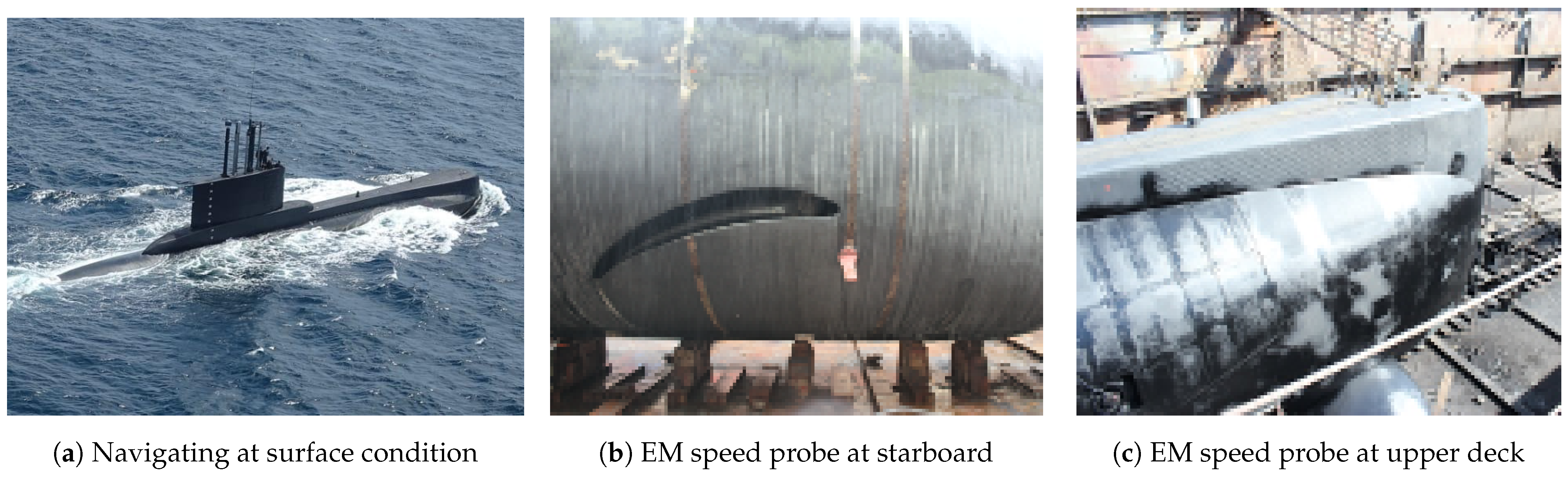
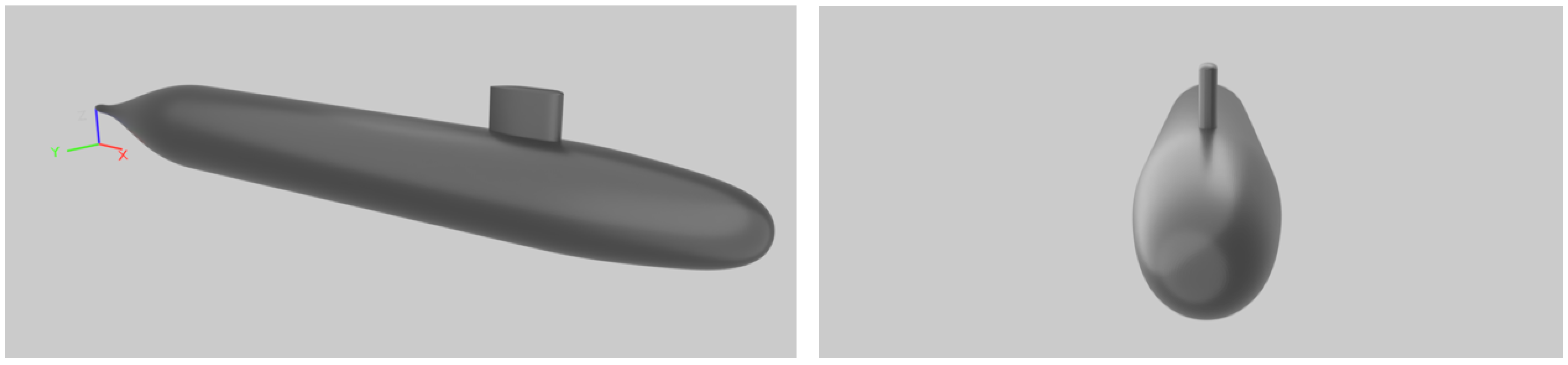
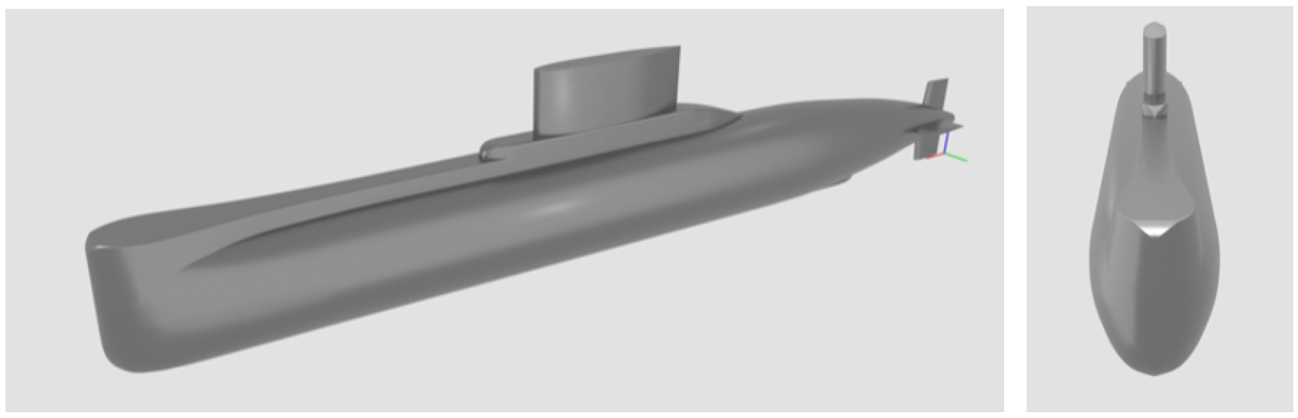
2.1. DARPA SUBOFF and Type 209/1300 Submarine Geometry

As described above, the geometry of the DARPA SUBOFF model is defined by polynomial equations [31] and consists of an axi-symmetrical hull tested in eight different arrangement configurations (AFF) depending on the appendages included [3]. In the present study, only the geometry of the bare hull with the sail is modelled because log probes are typically fitted on the forward half of the hull to avoid stern appendages or propeller interaction. Hence, the experimental resistance force data measured in the DTMB Tow Tank that is used in the validation is estimated from AFF-1 (bare hull), AFF-3 (hull with four stern appendages), and AFF-8 (hull with sail and four appendages).

On the other hand, Type 209 submarine is a diesel-electric warcraft built by HDW of Germany since 1971, with 61 units still operating in 13 countries worldwide. There are five variants depending on the surface displacement, from 1100 to 1500. In the last decade, most of the oldest submarines have being refitted including electronic equipment upgrades. In particular, the $209/1300$ submarine analyzed in this study upgraded to two EM speed logs, located at starboard and upper deck, see Figure 1, that must rely on experimental or numerical hydrodynamics studies to determine its light hull location and further calibration curve for near-surface and deep-water navigation.

This calibration curve is estimated from sea trials to guarantee the accuracy of the readings reported by the probes. This curve compares the submarine navigation speed and local flow velocity at probe location to compensate non-linearities for hydrodynamic variations produced by the curvature of the hull. In the submarine case, two calibration curves, near-surface and deep-water operation conditions, are used. Typically, the calibration of the deep-water curve uses the near-surface one as the reference navigation speed. However, this heuristic methodology wrongly assumes that flow at deep-water and near-surface conditions are similar, despite experimental evidence proving otherwise, as previously discussed. One alternative to quantify free surface effects at the full-length scale at regions near probe locations is to use an open-access experimental database, such as DARPA SUB-OFF. However, there are significant differences in displacement and length proportions with the 209/1300 class, as shown in

Table 1. Main characteristics comparison between DARPA–SUBOFF and Type 209/1300 submarines.

Parameter	Symbol	SUB-OFF Model Scale	SUB-OFF Equivalent Prototype Scale	Type 209/1300
Length between perpendiculars [m]	L	4.356	58.167	58.167
Length-Diameter ratio	$L/D$	8.575	8.575	9.950
Draft-Diameter ratio	$T/D$	0.863	0.863	0.863
Length percentage of fore body	$L_{FB}/L$	0.233	0.233	0.189
Length percentage of parallel middle body	$L_{PMB}/L$	0.512	0.512	0.496
Length percentage of aft body	$L_{AB}/L$	0.255	0.255	0.314
Relative sail location	$L_{FC}/L$	0.21	0.21	0.40
Wetted area of hull at surface [m2]	$S_{surf}$	4.760	848.759	775.220
Wetted area of hull + sail [m2]	$S_{hull-Sail}$	6.160	1098.394	1182.420
Wetted surface area of sail [m2]	$Ssail$	0.184	32.855	83.258
Displacement at surface condition [tons]	${\Delta }_{surf}$	0.650	1547.675	1309.950
Displacement submerged hull + sail [tons]	${\Delta }_{sub}$	0.703	1674.560	1578.00

, that prevent a straight forward extrapolation. Hence, the only feasible option is to perform a numerical study at full-scale to characterize flow conditions around the Type 209/1300 submarine light hull.

Finally,

Table 2. Control points locations measured from baseline used to probe flow velocity on the hull of a Type 209/1300 submarine.

Control Point	X (m)	Y (m)	Z (m)
P1	53.82	−2.34	1.34
P2	50.64	−0.53	7.02
P3	53.82	−2.68	1.14
P4	50.64	−0.53	7.41

shown the coordinates of four points, P1 to P4, that corresponds to the base and measurement location of fixed protruding probes at starboard (P1, P3) and upper deck (P2, P4), as shown in Figure 1. The distance between each pair of points is 40 cm, corresponding to distance between the probe base and its measurement position. This control points are used to assess the lineal variation of the local flow speed with navigation speed.

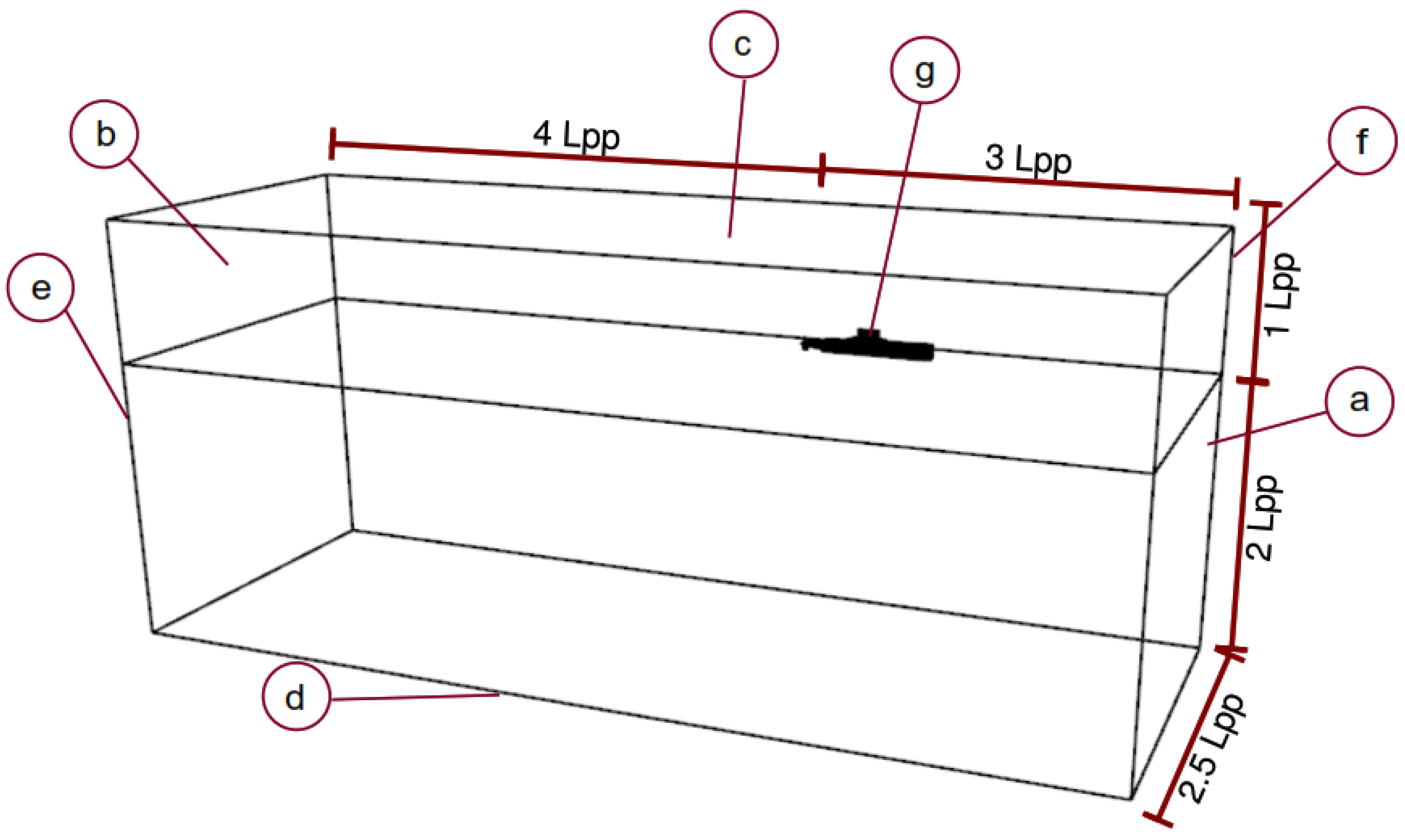
2.2. Simulation Setup for Submarines

For the DARPA SUBOFF-5470 submarine, the bare hull and sail configuration at model scale was considered, as shown in Figure 2. The hull is Axis-symmetric and is defined by polynomials as described in Groves et al. [31]. The 3D CAD geometry was generated using the Grasshopper plugin in Rhinoceros and the surface was exported to OpenFOAM as an STL file. Additionally, after transforming the geometry to mesh type, the water tightness of the geometry was verified with the software Blender.

For the Type 209/1300 submarine, a complete CAD model was generated by combining original blueprints provided by shipowner and measurements taken during a scheduled dry-dock maintenance. However, appendages with dimensions smaller than 10 cm such as: hydroplanes, passive sonars, antennas, and collision bumpers, were not included in the CAD version used in the current work. This simplified CAD version, shown in Figure 3, was used in the numerical simulations to decrease the required computational time per simulation, where neither propeller geometry nor its hull interaction is included.

Although the flow around the submarine may be vortex dominated, the dominant vortical structures are generated by the sail [32], that produce asymmetrical flow structures about the central plane that are shed downstream along the hull, hence requiring a full-domain approach. Nevertheless, there is evidence that when a submarine is moving straight-ahead, it is possible to use the half-domain approach [5,7,10,21]. On the other hand, if the submarine propeller [9,17], self-propulsion problem [12,13,14,18,26], or maneuvering characteristics [27,29] are numerically assessed; then a full-domain approach must be used. The present work focus on the forward hull region below the free surface interface, where the flow is expected to be axisymmetric when fully submerged as reported by Lungu [6], that is slightly perturbed by the occurrence of breaking wave in front of the bow due to vertical, cylindrical bow that is symmetric around centerline when operating at surface depth, as reported by Jasak et al. [33]. Thus, half-domain approach is chosen in this work and decreasing the required time per simulation.

Hence, the computational domain size was defined following ITTC guidelines [34], where the inlet, side, bottom, atmosphere, and outlet boundaries are placed far enough from the submarine to avoid spurious flow interaction, see Figure 4. The boundary conditions are shown in

Table 3. Boundaries names and conditions.

Label	Name	U	$\mathit{p}\_\mathit{rgh}$
a	Inlet	fixedValue	fixedFluxPressure
b	Side	symmetryPlane	symmetryPlane
c	Atmosphere	pressureInletOutletVelocity	totalPressure
d	bottom	fixedValue	fixedFluxPressure
e	outlet	outletPhaseMeanVelocity	zeroGradient
f	midPlane	symmetryPlane	symmetryPlane
g	hull	movingWallVelocity	fixedFluxPressure

for all patches of the computational domain, where the no-slip wall condition is imposed on the submarine boundary. Regarding initial conditions, the flow velocity is initialized with the navigation speed in the inlet, bottom, and internal field. In addition, turbulent kinetic energy ($\kappa$) and its specific rate of dissipation ($\omega$) are set assuming a turbulence intensity level of $1.5\%$ considering wall functions for the hull patch.

The computational grids are generated in stages: (i) an hexahedral background grid using blockMesh with refinement in the region where free-surface interface is expected, (ii) six refinement levels using topoSet tool to half the element size progressively as the elements get closer to the submarine hull, (iii) the surface is inserted with additional (1 or 2) refinement levels if the elements is less than 0.1 D from the submarine hull, (iv) eight layers of prismatic elements parallel to submarine surface are included with a target yPlus, that is estimated considering the laminar boundary layer thickness as a reference length to capture boundary layer evolution efficiently. Figure 5 shows slices of centerline showing one of the generated grids for SUBOFF and S209 submarines. The progressive refinement in regions close to the submarine is evident, aiming to capture high gradients of velocity in the boundary layer and pressure distribution around the submarine’s light hull.

Table 4. Number of cells for uncertainty analysis.

#	Grid Type	DARPA SUBOFF	Type 209/1300
1	Finer	11,986,756	22,832,329
2	Fine	4,500,437	9,145,512
3	Medium	1,576,885	3,892,550
4	Coarse	600,071	1,348,794
5	Coarser	215,582	514,008

shows the number of cells used for modelling the computational domain to estimate grid errors and uncertainties. The element size in the inner topoSet region is used as the reference length ($\Delta x$) and it is uniform in all three directions to improve the reliability of free surface evolution and turbulence prediction. The Medium grid was generated using the ITTC recommendations and the additional grids were generated using a refinement ratio of $rG=\sqrt{2}$ in both directions. For the Medium grid: (i) DARPA SUBOFF, an element size close to the submarine of 0.05 m ($L/\Delta x=87.12$) and a target yPLus of 50 were used, (ii) Type 209/1300, an element size of 0.20 m ($L/\Delta x=291.45$) and a target yPLus of 300 were used. For the second geometry, the element size is of the same order of magnitude than the probe dimension and it will capture the relevant flow characteristics for speed log accuracy.

Figure 6 shows the distribution of the number of surface layers obtained for each of the considered meshes, despite having requested eight layers, suggesting that most of the hull has the necessary elements to capture the viscous effects within the boundary layer. This difference is due to the mesh quality parameters and curvature of the light hull at the bow and stern sections. Despite the above, the prism surface layer reaches the requested thickness in most of the outer hull, not shown here. Although the yPlus distribution near the surface at the bow, sail, and aft regions has values greater than 300, it is expected that it will not affect the main flow characteristics near the probe location due to its small influence area.

2.3. Test Matrix

The DARPA SUBOFF submarine was used for the Verification and Validation considering $H/D=5.4$ and $Fr=0.46$ condition, where H is the distance from the free-surface to the hull diameter centerline. The numerical prediction is compared to the experimental data provided by Liu and Huang [3]. Additional simulations predictions using the verified grid were compared with the experimental data provided by Neulist [35] for different immersion depth $H/D$ ratios and Froude number, as shown in

Table 5. Experimental data used for Verification and Validation of DARPA–SUBOFF submarine simulations.

H/D	Fr	${\mathit{C}}_{\mathit{T}}\times {10}^3$	Source
	0.132	4.730
1.1	0.310	5.980	Neulist [35]
	0.463	7.440
	0.132	4.460
2.2	0.310	3.690	Neulist [35]
	0.463	4.110
5.4	0.466	3.310	Liu and Huang [3]

:

For the Type 209/1300, the navigation conditions shown in Figure 7 were used to assess the flow characteristics, free-surface effects, and potential zones on the light hull of the submarine for probe installation to guarantee measurement accuracy fulfilling the manufacturer requirements. Thus, three different drafts measured at the aft perpendicular were considered without initial trim, namely: (i) surface depth at 5.18 m, (ii) periscope depth at 12 m, and (iii) deep-water at 40 m corresponding to a non-dimensional $H/D$ of 0.33, 1.47, and 6.14 respectively.

Table 6. Parameters used in each of the simulations in the present study of the Type 209/1300 submarine.

Simulation	Navigation Condition	Velocity [Knots]	Coarse Grid	Intermediate Grid	Fine Grid
1–3		9.0	X	X	X
4	C1: Surface depth	6.0			X
5		3.0			X
6		9.0			X
7–9	C2: Periscope depth	6.0	X	X	X
10		3.0			X
11		9.0			X
12–14	C3: Deep-water	6.0	X	X	X
15		3.0			X

shows the navigation details for each Type 209/1300 simulation performed in the present study, such as velocity, draft, and grid density considering operational limits reported by the submarine crew. First, simulations 1–3 were used to assess grid convergence independence with the submarine navigating at 9 knots ($Fr=0.194$) at surface depth and no trim. Later, simulations 7–9 and 12–14 are completed to confirm grid convergence study navigating at 6 knots ($Fr=0.129$) at periscope and deep-water depths respectively. Additional simulations with the submarine at conditions 1, 2, and 3 were used to verify the linear variation of the local speed measured by the probe including a speed of 3 knots (Fr = 0.065).

3. Results

The numerical results obtained with the settings described in the previous section are summarized here. First, a Verification and Validation procedure is performed using the DARPA SUBOFF submarine geometry at model scale. Next, the grid sensitivity at full-scale was assessed using the total resistance predictions acting on the Type 209/1300 submarine sailing at three navigation conditions: surface depth, periscope depth, and deep-water immersion depth, considering the recommendations described by [1,33,36,37]. Later, the flow was characterized considering the fine grid by assessing the flow around the external hull, wave train, dynamic pressure, yPlus, and wall Shear Stress distribution, and visualization of vortex cores following [38,39].

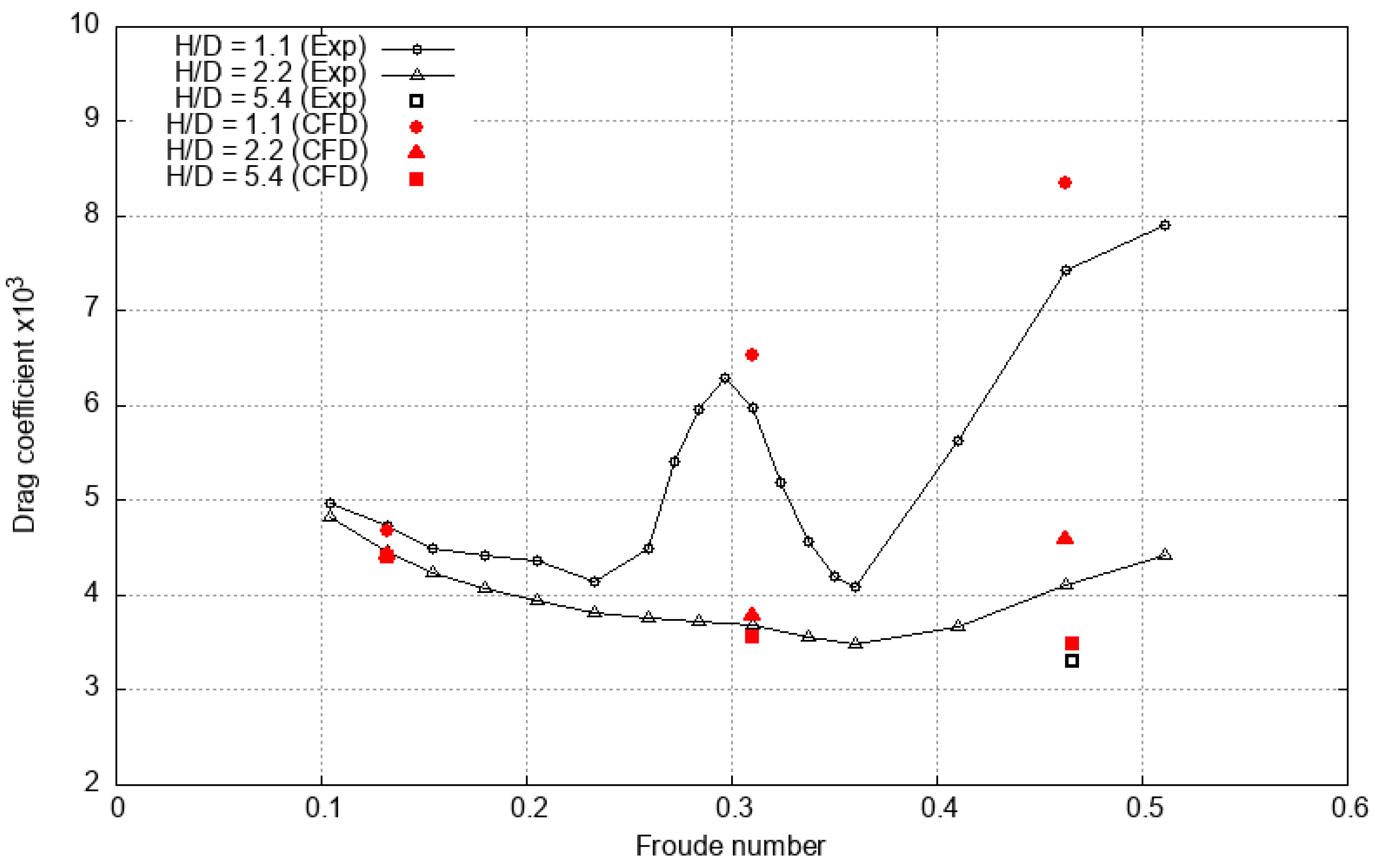
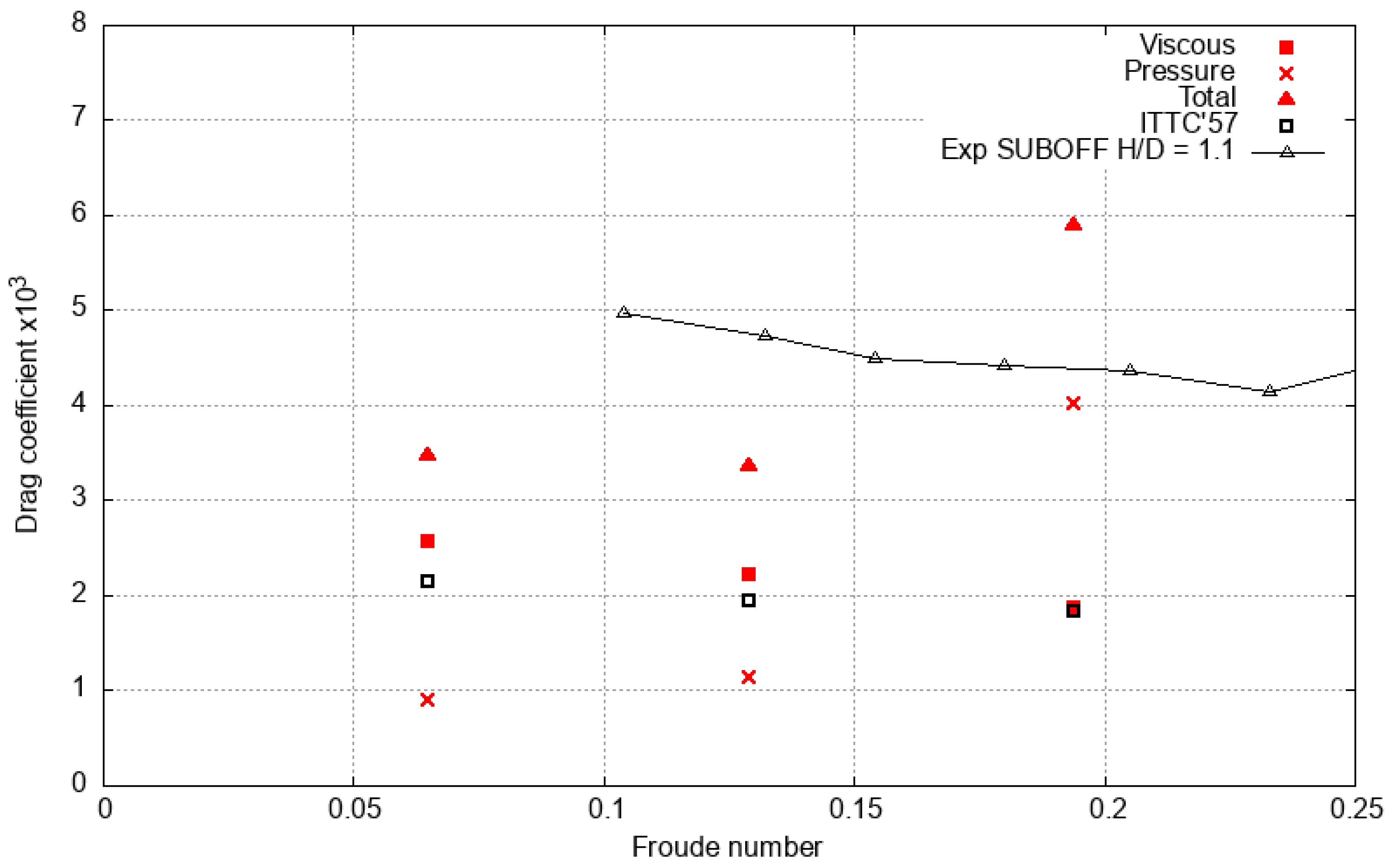
3.1. Verification and Validation

For this procedure, simulations were performed considering the navigation conditions, $H/D=5.4$ and $Fr=0.466$, previously described in Table 5. Figure 8 shows: the evolution of: (i) the residual for dynamic pressure, the fraction of water, $\kappa$, and $\omega$ variables and (ii) viscous and pressure force components acting on the hull, both for the previously described navigation condition using the fine grid with 4,500,437 cells. All residuals smoothly decreased several orders of magnitude, but the dynamic pressure oscillates around ${10}^5$. Also, both force components achieved convergence after 2000 time steps, which could be related to the absence of free-surface effects. The others grids show the same behaviour.

Figure 9 shows the evolution of the resistance force for all grids. It is evident that convergence is achieved after 2000 iterations. Additionally, all curves are smooth, but Grid 03 that has spurious oscillations. Grid 01 and 02 are close, suggesting that grid convergence have been achieved.

Table 7. Average and standard deviation of force components vs grid density for SUB-OFF submarine at $Fr=0.466$ and $H/D=5.4$.

Grid Density	Number of Cells	Pressure	Viscous	Total	% SD	Exp Value	% Error	Avg. $\mathit{y}+$
Coarser	215,582	30.840	82.840	113.685	0.004		20.6%	103.24
Coarse	600,071	21.643	86.270	107.913	0.009		14.4%	58.29
Medium	1,576,885	17.631	86.271	103.902	0.798	94.29	10.2%	43.39
Fine	4,500,437	12.508	86.954	99.461	0.002		5.5%	23.06
Finer	11,986,756	10.884	87.813	98.696	0.097		4.7%	16.48

shows the average values of pressure and viscous force components acting on the whole hull area, and it is estimated as two times the average of the last 1000 iterations for each grid considered in this study. Although the numerical prediction approximates to the experimental value and the error percentage decreased considerably from Grid 05 to 01, it is still at 4.7% for the latter. It is believed that a possible explanation of the current simulations is due to the existing limitations of snappyHexMesh to add enough prism layers in about 1.1% of the hull area, especially on the hull-sail intersection and the aft end of the hull. Another source of error is from the procedure estimation of the experimental data, since the hull-sail configuration is obtained from three different configurations (AFF1 + AFF8 - AFF3) as described in [3]. Further simulations of SUBOFF use the fine grid due to current hardware limitations.

Table 8. Total resistance coefficient convergence for SUB-OFF submarine at $Fr=0.466$ and $H/D=5.4$.

Grid	Coarser—G5	Coarse—G4	Medium—G3	Fine—G2	Fine—G1	Richardson Extrapolation	Exp Value—S
$C_T\times {10}^3$	3.985	3.783	3.642	3.486	3.460	3.433	3.305
$E\%$		5.1%	3.7%	4.3%	0.8%
${ϵ}_{ij}\times {10}^3$		0.202	0.141	0.156	0.027

and

Table 9. Verification and Validation parameters considering grids 1–5 for SUB-OFF submarine at $Fr=0.466$ and $H/D=5.4$.

Analysis Set	${\mathit{R}}_{\mathit{G}}$	$\%{\mathit{GCI}}_{\mathit{FINE}}$	${\mathit{P}}_{\mathit{G}}$	${\mathit{C}}_{\mathit{G}}$	${\mathit{U}}_{\mathit{G}}\%\mathit{S}$	${\mathit{\delta }}_{\mathit{G}}\%{\mathit{S}}_{\mathit{C}}$	${\mathit{U}}_{\mathbf{GC}}\%{\mathit{S}}_{\mathit{C}}$	${\mathit{S}}_{\mathit{C}}$
1–3	0.172	0.2%	4.98	4.842	1.4%	0.8%	0.6%	3.433
2–4	1.107
3–5	0.695	14.3%	0.90	0.433	8.9%	4.0%	2.7%	3.501

show the results of the Verification calculations obtained using the Total Resistance coefficient from the numerical results previously shown in Table 7. The convergence ratio $R_G$ of 0.172 and 0.605 means that the numerical results for these grid sets (1–3, and 3–5) are in the convergence region and Richardson extrapolation can be used to estimate the numerical force coefficient corresponding to a grid with infinity number of cells. For the grid 1–3 set, the low values of ${\delta }_G=0.8\%$ and $U_{GC}=0.6\%$ suggest that numerical results achieved grid convergence and it could be considered as verified.

Finally, Figure 10 compares numerical Total Resistance Coefficient prediction to the experimental values provided by Neulist [35] and Liu and Huang [3]. Although the numerical prediction seems to slightly over-predicts the Total drag coefficient for all $H/D$ ratios but for the lowest Froude number $Fr=0.132$, simulations are able to capture the non linear variations at intermediate Froude $Fr=0.31$ for the near-surface condition $H/D=1.1$. Furthermore, the difference at the lowest Froude condition could be explained by limitations on computational resources and should decrease further refining the grid.

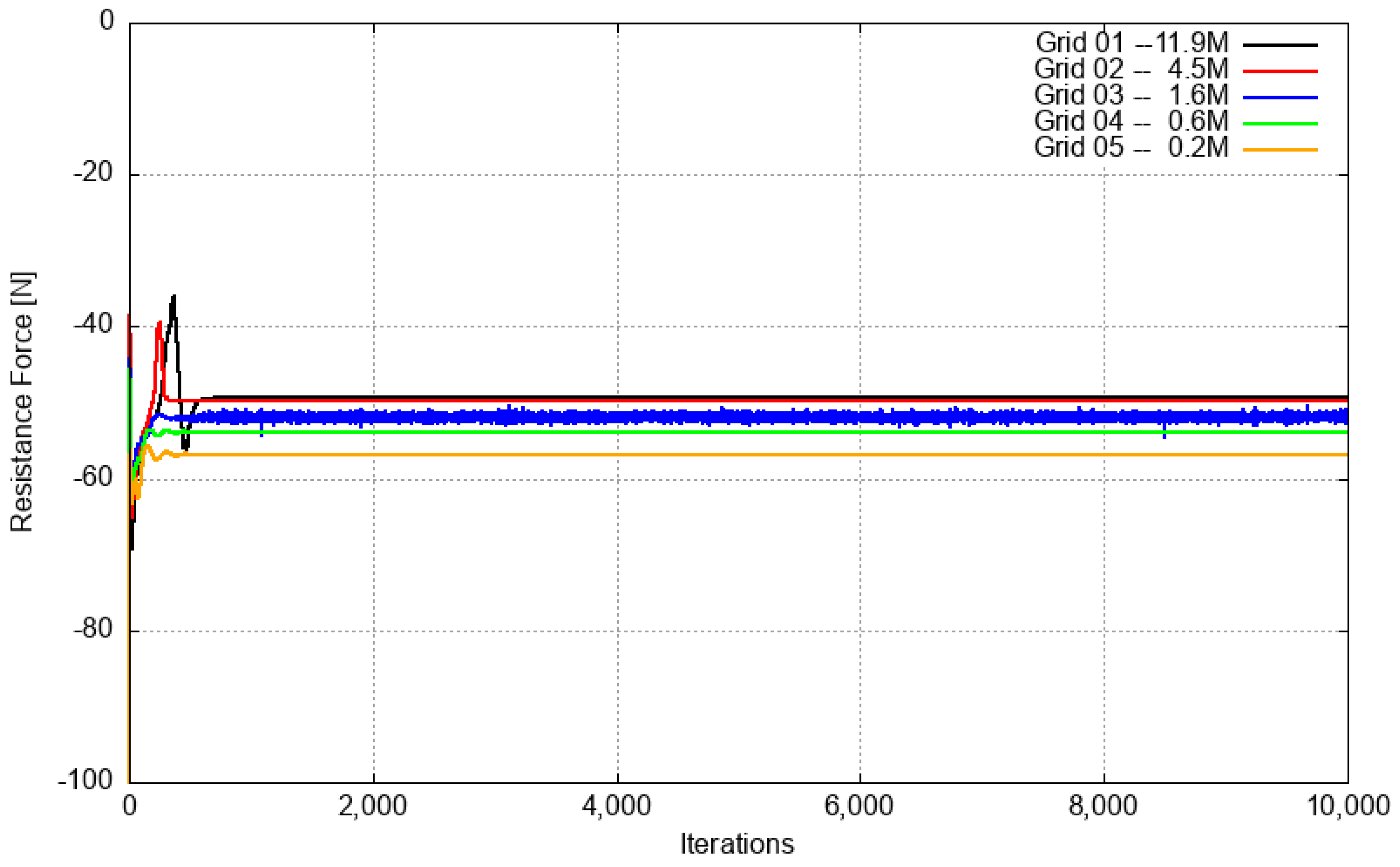
3.2. Grid Convergence for Type 209 at Full-Scale

Figure 11 shows the evolution of the viscous and pressure force components acting on the submarine light semihull for simulation 03 using $CFL=4$ in the fluid domain and free-surface interface taking advantage of the implicit MULES scheme. As usual, the viscous component is related to the shear stresses of both fluids and the pressure component is linked to normal stresses due to the interaction of fluid motion and waves generated around the submarine. Both resistance components reach steady values after 10,000 iterations, with a smoother behaviour for the coarser. Furthermore, the viscous curve converges faster, and it is smoother than the pressure curve, as expected. The force evolution predicted using coarse and intermediate grids shows a similar behavior but with an increased dispersion on the pressure curve, that is suspected to be produced by smaller vortices being captured, and spurious instability produced by high CFL number. For this reason, the smaller CFL number of 4.0 was chosen to avoid the occurrence of numerical instability. In summary, the viscous component represents roughly $30\%$ of the total resistance force, which agrees with the expected predictions of cylindrical bluff bodies moving near a free surface at moderate Froude numbers.

The viscous and pressure force predictions shown in

Table 10. Average and standard deviation of force components vs grid for submarine at condition 1 with Domain CFL = 4 and Free surface CFL = 4.

Grid Density	Number of Cells	Pressure (N)	Viscous (N)	Total (N)	SD (N)
Coarser	524,008	17,560.51	7390.06	24,950.57	446.85
Coarse	1,348,794	15,602.31	7927.64	23,529.95	336.51
Medium	3,892,550	16,467.29	7807.49	24,274.78	292.47
Fine	9,145,512	16,640.02	7768.89	24,408.91	450.07
Finer	22,832,329	15,709.69	8113.64	23,823.22	459.44

correspond to average values of the last 1000 iterations for each of the grids considered in Simulation 03, namely, $H/D=0.33$ and $Fr=0.194$. The standard deviation is used as an indicator of the variation between iterations of the total force, having a maximum value of almost 460 N (2% of average value) of the pressure component for the finer grid, that is similar to the behaviour described in Jasak et al. [33] where a transient simulation of a general cargo carrier shows the resistance force oscillating due to breaking waves in front of the bow.

Figure 12 shows the iteration evolution of the total resistance for grids 01 to 05. All curves seem to achieve a quasi-steady state value with oscillations that could be related to the bow breaking wave shown in Figure 13. In this study, convergence condition ($R_G$) is calculated as 0.18 for the Grid set 2–4 which means that the solution is converged monotonically. For Grid sets 1–3 and 3–5, $R_G$ is calculated as −4.366 and −0.524 respectively, which means that the solution has an oscillating convergence. The Grid Convergence Index (GCI) for the set 2–4 is $1.0\%$, $0.3\%$, and $3.9\%$ for sets 1–3, 2–4, and 3–5, where the latter has the higher uncertainty. Furthermore, the total resistance is extrapolated from set 2–4 using the Richardson extrapolation procedure [37] to 24,458.84 N for an infinite number of elements. Hence, the fine grid is considered as acceptable considering its balance between the resolution of the flow characteristics and the required computational resources. All remaining simulations will use this fine grid with 9,145,512 elements.

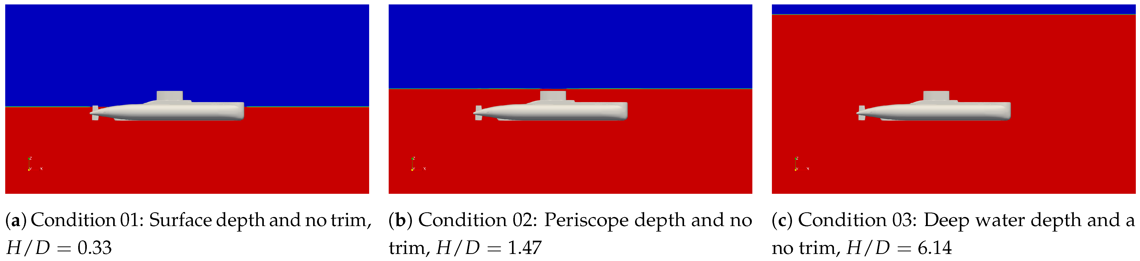
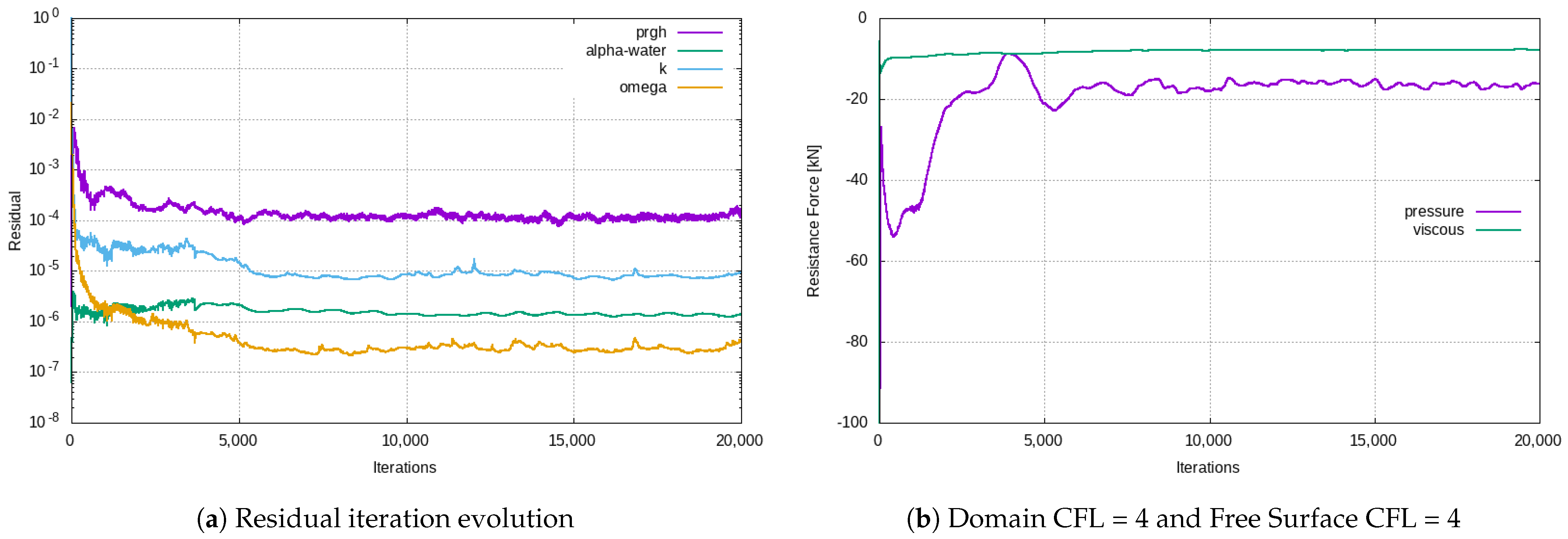
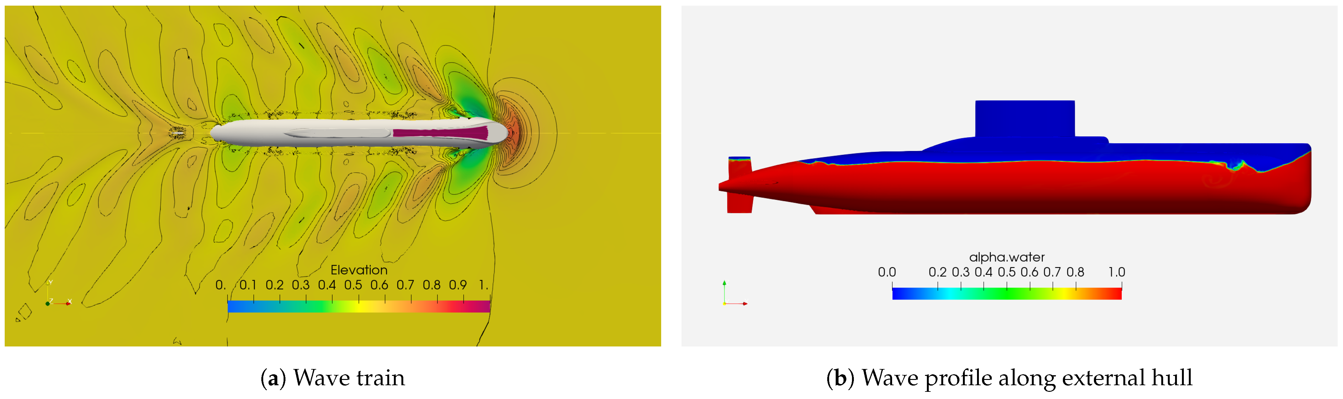
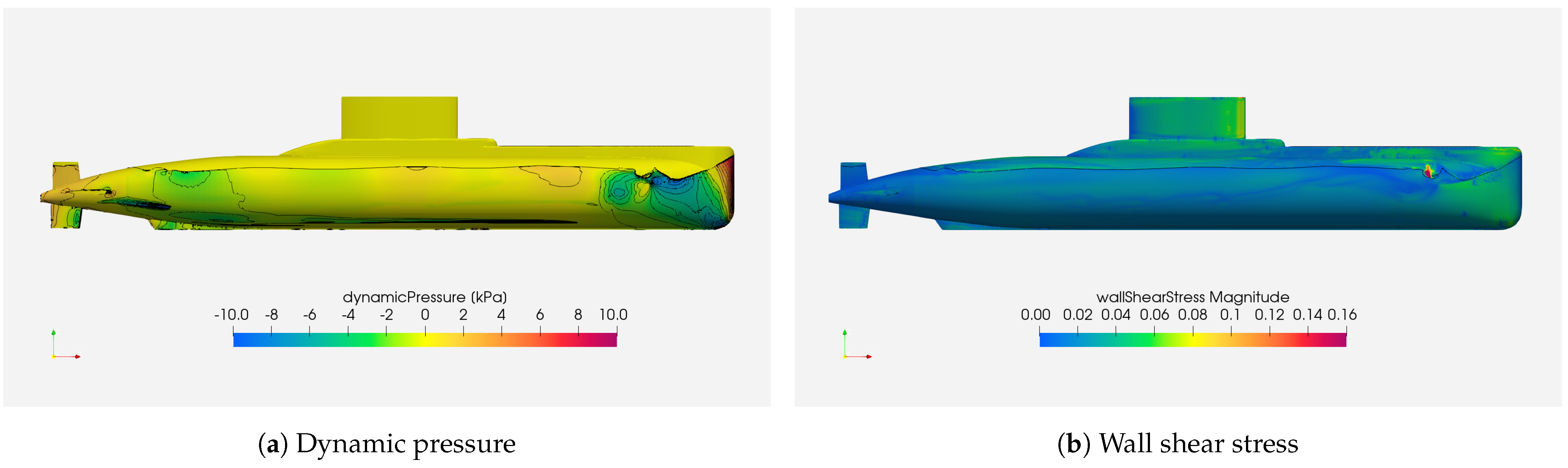
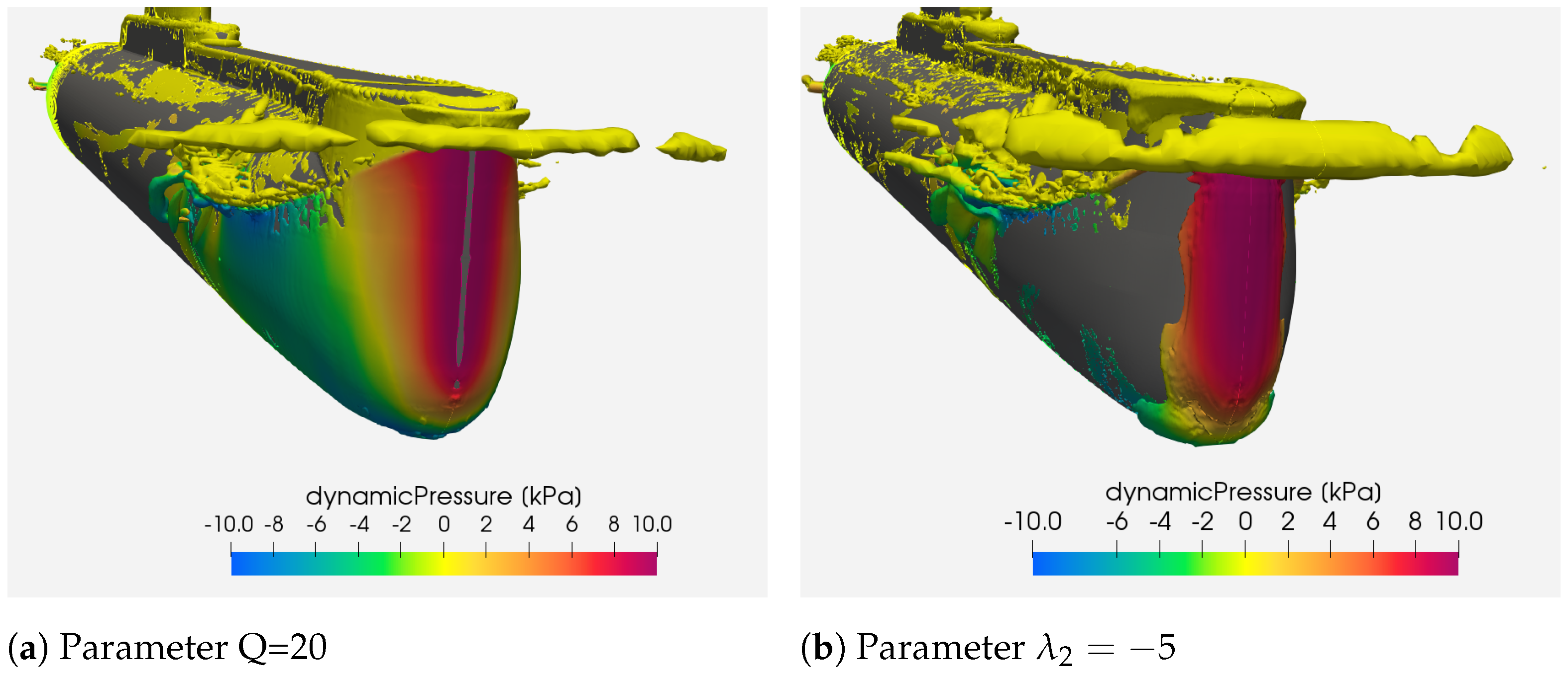
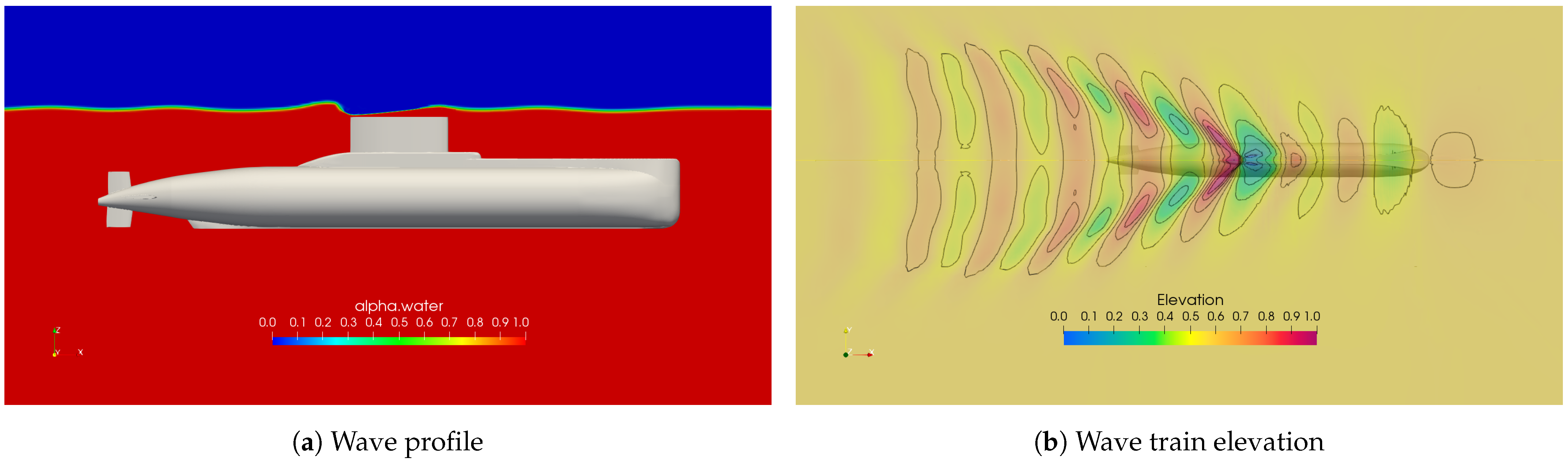
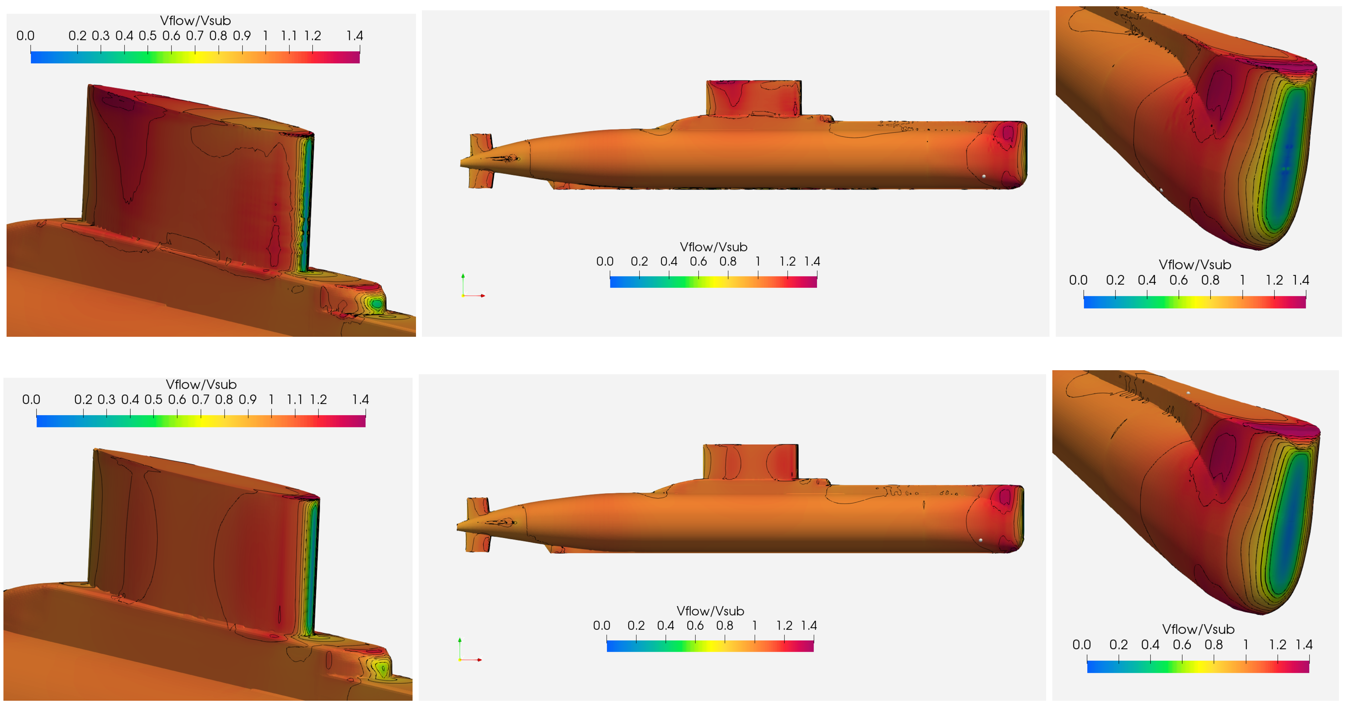
3.3. Flow Characterization at Condition 01: Surface Depth—H/D = 0.33

Figure 13 shows the wave train generated around the Type 209/1300 submarine at condition 1, namely, $H/D=0$ and $Fr=0.194$. On the left-hand side, it is evident that two Kelvin wave patterns are obtained, regardless of a spurious green water on the submarine upper deck produced by the instantaneous acceleration imposed as initial condition. Regarding both wave systems: (i) the system beginning at the submarine’s bow with a 0.4 m wave amplitude forward stagnation point, and (ii) the small system beginning at the higher aft foil with a 0.2 m wave amplitude. On the right-hand side, the water fraction distribution profile shows that the first wave crest is almost high enough to wet the upper deck area. However, the next wave trough is modified by a small wave system generated at the upper deck and light hull intersection. The wave profile seems to be canceled after this area as the flow moves downstream, in agreement with the theoretical prediction of the first wave resistance hollow.

Figure 14 shows the dynamic pressure and wall shear stress distribution around the Type 209/1300 submarine at condition 1 and $Fr=0.194$. On the right-hand side, it is possible to distinguish a stagnation area at the bow of the forward body section as predicted by a Pitot-tube like device and several pairs of high-low pressure areas produced by wave crest-trough propagation. Moreover, there are stagnation areas at the nose of each aft foil. On the left-hand side, the wall shear stress distribution seems smooth, but in the near-surface bow region at the bow wave trough, where high gradients are observed and the presence of turbulent eddies at the free surface level is suspected.

Figure 15 shows the flow velocity distribution relative to the navigation speed of the submarine including contour lines between 0.5 and 1.3. The stagnation area at the submarine bow described earlier is followed by a wide high-velocity gradient area where, in principle, the speed probe should not be fitted. Moreover, a small high velocity region is revealed at the first wave trough described before that could be related to vortices being shed from this location. Although P1, corresponding to the side probe base location (marked by a grey dot), is at the end of the acceleration region on a wide velocity region where the local flow speed is between 1.1 and 1.2 times higher than the navigation speed. Velocity probe could be installed here, because of appendage restrictions, if the local flow velocity remains inside this range for the whole range of operational speeds. Hence, it is required to include the results from Simulations 04 and 05.

Figure 16 shows the local flow velocity as a function of navigation speed at two locations: P1 and P3, corresponding to the measurement position of a protruding probe that is 40 cm away from P1. Both trend lines for condition 01 can be approximated by a lineal function with a slope of 1.15, which suggests that the flow velocity remains in the 1.1–1.2 range described before and that there is not a significant difference in local flow if measured by a flush or protruding probe when the boundary layer effect is neglected.

Figure 17 shows vortex cores at the submarine bow identified by using Q and ${\lambda }_2$ parameters. Both methods detect a dominant vortex structure at the bow wave and its downstream propagation along the light hull. Small vortex structures with low dynamic pressure (high flow velocity) are detected at the free surface level near the first trough wave, as suggested by the wall shear stress distribution shown above. The latter method is able to detect smaller structures at the free surface and upper deck level.

Finally, Figure 18 shows the numerical prediction of drag coefficients for total, viscous, and pressure force components as a function of Froude number, including ITTC’57 curve for the submarine at condition 01 and Total Drag Coefficient for SUBOFF at $H/D=1.1$. The total coefficient prediction of the Type 209/1300 submarine has a different behaviour than the SUBOFF, and it is closer to the variation expected for surface vessels. Viscous coefficient data compares well with ITTC’57 curve despite its light hull has fuller form than standard surface vessels. Furthermore, the pressure component, which includes wave-making and form factor effects, increases with Froude number as expected, and becomes dominant for higher Froude number. The viscous coefficient difference could be related to insufficient elements being used to describe the hull surface for lower Froude numbers.

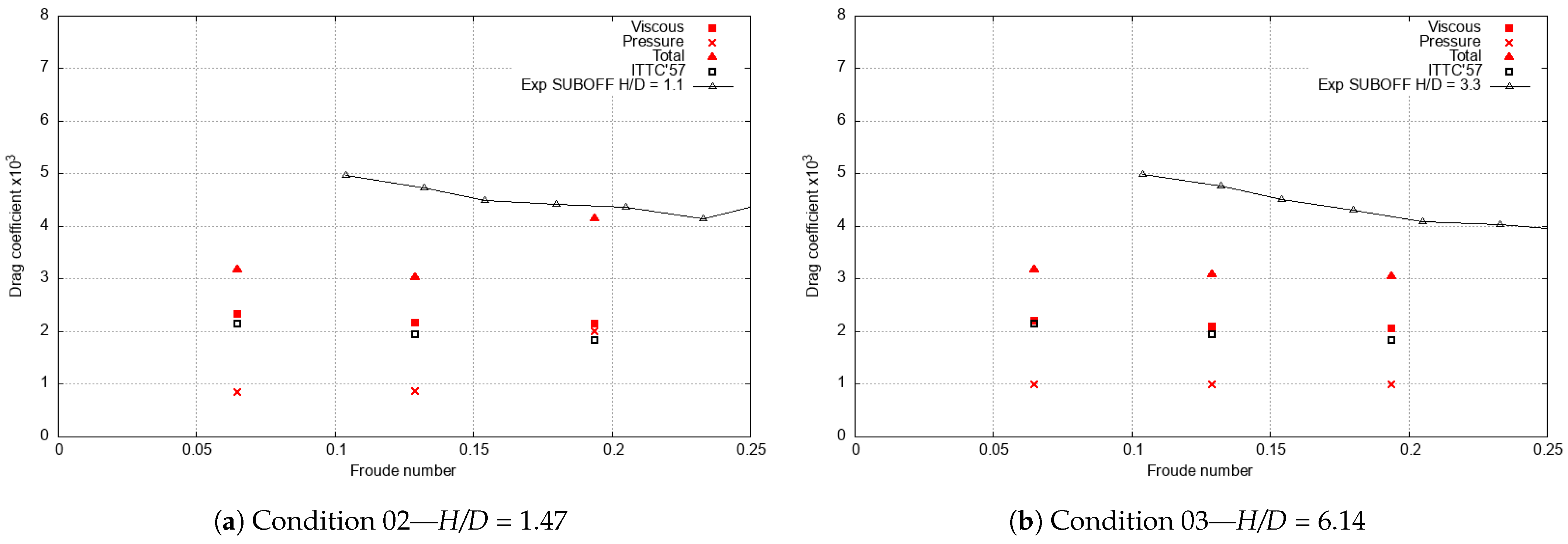
3.4. Free-Surface Depth Influence on Flow Characteristics

Figure 19 shows the wave profile at midplane generated by the Type 209/1300 submarine navigating at $H/D=1.47$ and $Fr=0.194$. On the left-hand side, the sail deforms the free surface above it due to a Venturi effect and produces a short length wave system beginning at the sail end regardless of no free surface piercing. On the right-hand side, the wave elevation demonstrates a weak free-surface interaction with the submarine light hull, where a small wave amplitude system is generated.

Figure 20 shows the flow velocity distribution on light hull relative to the submarine speed including contour lines between 0.5 and 1.3 for H/D = 1.47 and 6.14. In both conditions, the stagnation area at the submarine’s bow, sail, and aft foils are followed by a high-velocity gradient where the probe should not be installed. On the other hand, P1—side probe base, marked by a grey dot, is located on a wide velocity region between 1.1–1.2 times the navigation speed and P2—upper deck probe base in on a slower region between 1.0–1.1 times the navigation speed is used when the submarine is completely submerged. Hence, speed probes could be mounted on both locations given the local flow velocity remains this range for the whole range of operational navigation speeds regardless of its difference with the condition 01 H/D = 0.33. Moreover, the calibration procedure used for the upper deck probe is discouraged because it is located on a different velocity range. Finally, the flow velocity distribution is similar for H/D = 1.47 and 6.14 but at the sail produced by its free surface proximity where changes are evident at the sail side.

On the left-hand side, Figure 21 shows local flow velocity as a function of navigation speed at two locations: P1 and P2 for $H/D=1.47$. Both trend lines can be approximated by linear functions with a slope of 1.12 and 1.03 respectively, suggesting that the local flow velocity around the side probe at P1 remains in the 1.1–1.2 range predicted for the surface depth condition and that it is safe to use this probe when the submarine is operating at near-surface condition. On the other hand, the upper deck probe at P2 is within a different speed range 1.0–1.1, suggesting that the calibration procedure based on the side probe is not appropriate producing an error of 0.25 knots when the submarine is navigating to 9 knots ($Fr=0.194$). On the right-hand side, the local flow velocity at P1 is shown as a fraction of the navigation speed. The local flow velocity decreased almost $4\%$ when the submarine move from emerged ($H/D=0.33$) to the deep-water condition ($H/D=6.14$) slightly increasing the error of the measured velocity by side probe sensor.

Finally, Figure 22 shows drag components coefficients as a function of Froude number, including the ITTC’57 curve for submarine at $H/D=1.47$, and $H/D=6.14$ conditions and the Total Drag Coefficient for SUBOFF at $H/D=1.1$ and $H/D=3.3$. On the right-hand side, viscous coefficient data compares well with the ITTC’57 curve, despite the wetted area includes the sail contribution. The pressure component is almost parallel to the viscous one, suggesting that the form factor could be estimated. Total drag coefficients have the same trend as the experimental values for SUBOFF geometry at $H/D=3.3$, where some free surface effects are still present. On the left-hand side, viscous data have the same behavior as before, and pressure data seems to increase as the Froude number increases. The Wave-making coefficient could be estimated by deducting the form factor previously estimated.

4. Conclusions

Results for DARPA SUB-OFF geometry demonstrate that the numerical methodology used in this work is reliable at the engineering level when 4,500,000 cells are used in the simulations. The Verification and Validation procedure was used to estimate the numerical uncertainty of three grid sets combining 5 different densities. Also, strong nonlinear effects due to proximity to free-surface can be captured for Froude number of $Fr=0.3$ at $H/D=1.1$.

Considering the results and discussion shown in the previous section, it is concluded that the side probe sensor could be installed at P1 location considering that this area presents a continuous flow without recirculating zones or vortex cores for all the navigation conditions considered. However, turbulent structures are concentrated in the near-surface regions. This probe will be located close to the end of the acceleration region at bow, where the local flow speed is still 15% higher than actual submarine speed. This location is recommended to be used when submarine is at surface condition because the flow is considered linear because its velocity remains at the same level for navigation velocities between 0 and 9 knots. Moreover, speed measurements could be useful for near-surface and deep-water conditions if a 4% correction is included to compensate for free-surface effect. On the other hand, the current calibration procedure used for the upper deck probe at P2 using the side probe measurement at P1 as a reference should be further modified to take into account the difference in the flow velocity range of both locations P1 and P2.

Finally, it is recommended to verify the effect of boundary layer thickness on speed measurements of the flush probe type to guarantee the expected accuracy of the flush probe and to generate validation data during sea trials, including at least 8 calibration points for the flush probe type to compensate the manufacturer declared difference in precision (±0.2 knots) between flush and protruding probe types.

This research could follow several interesting paths: (i) to improve results reliability, authors could perform transient simulations, include ramping initial conditions, improve the prism layer generation to cover 100% of the submarine hull, include a wave damping region at the outlet boundary to avoid reflections; (ii) to assess the non-linear free surface effect for Froude numbers between 0.2 and 0.4, to assess the boundary layer thickness effect on speed measurements or assessing the operational trim effect on flow characteristics. Finally, it will be challenging to assess the Type 209 submarine in self propulsion or maneuvering conditions.

References

1. ITTC. Uncertainty Analysis in CFD Verification and Validation Methodology and Procedures. In ITTC—Recommended Procedures and Guidelines; 28th ITTC Executive Committee: Wuxi, China, 2017; Chapter 7.5-03-01-01. [Google Scholar]
2. Stern, F.; Wilson, R.; Shao, J. Quantitative V&V of CFD simulations and certification of CFD codes. Int. J. Numer. Meth. Fluids 2006, 50, 1335–1355. [Google Scholar] [CrossRef]
3. Liu, H.L.; Huang, T.T. Summary of DARPA SUBOFF Experimental Program Data; Technical Report CRDKNSWC/HD-1298-11; Naval Surface Warfare Center, Carderock Division (NSWCCD): West Bethesda, MD, USA, 1998. [Google Scholar]
4. Huang, T.T.; Liu, H.L.; Groves, N.C. Experiments of the DARPA SUBOFF Program; Technical Report DTRC/SHD-1298-02; Davidson Taylor Research Center: Bethesda, MD, USA, 1989. [Google Scholar]
5. Gross, A.; Kremheller, A.; Fasel, H. Simulation of Flow over SUBOFF Bare Hull Model. In Proceedings of the 49th AIAA Aerospace Sciences Meeting including the New Horizons Forum and Aerospace Exposition, Orlando, FL, USA, 4–7 January 2011; American Institute of Aeronautics and Astronautics: Orlando, FL, USA, 2011. [Google Scholar] [CrossRef]
6. Lungu, A. DES-based computation of the flow around the DARPA suboff. IOP Conf. Ser. Mater. Sci. Eng. 2019, 591, 12053. [Google Scholar] [CrossRef] [Green Version]
7. Vasileva, A.; Kyulevcheliev, S. Numerical Investigation of the Free Surface Effects on underwater vehicle resistance. In Proceedings of the Fourteenth International Conference on Marine Sciences and Technologies, Varna, Bulgaria, 10–12 October 2018; Black Sea: Varna, Bulgaria, 2018; pp. 100–104. [Google Scholar]
8. Gourlay, T.; Dawson, E. A Havelock source panel method for Near-surface Submarines. J. Mar. Sci. Appl. 2015, 14, 215–224. [Google Scholar] [CrossRef] [Green Version]
9. Di Felice, F.; Felli, M.; Liefvendahl, M.; Svennberg, U. Numerical and experimental analysis of the wake behavior of a generic submarine propeller. In Proceedings of the First Internationnal Symposium on Marine Propulsors, Trondheim, Norway, 22–24 June 2009; p. 7. [Google Scholar]
10. Takahashi, K. Numerical Simulations of Comprehensive Hydrodynamics Performance of DARPA SUBOFF Submarine. Master’s Thesis, Florida Institute of Technology, Melbourne, FL, USA, 2019. [Google Scholar]
11. Liefvendahl, M.; Troëng, C. Computation of Cycle-to-Cycle Variation in Blade Load for a Submarine Propeller, using LES. In Proceedings of the Second International Symposium on Marine Propulsors, Hamburg, Germany, 15–17 June 2011; p. 7. [Google Scholar]
12. Chase, N. Simulations of the DARPA Suboff Submarine Including Self-Propulsion with the E1619 Propeller. Master’s Thesis, University of Iowa, Iowa City, IA, USA, 2012. [Google Scholar] [CrossRef] [Green Version]
13. Dogrul, A.; Sezen, S.; Delen, C.; Bal, S. Self-propulsion simulation of DARPA suboff. In Proceedings of the 17th International Congress of the International Maritime Association of the Mediterranean (IMAM 2017), Lisbon, Portugal, 9–11 October 2017; Maritime Transportation and Harvesting of Sea Resources, Tecnico Lisboa: Lisbon, Portugal, 2017; Volume 1, pp. 503–511. [Google Scholar]
14. Delen, C.; Sezen, S.; Bal, S. Computational Investigation of Self Propulsion Performance of Darpa Suboff Vehicle. Tamap J. Eng. 2017, 2017, 4. [Google Scholar]
15. Moonesun, M.; Javadi, M.; Charmdooz, P.; Mikhailovich, K. Evaluation of submarine model test in towing tank and comparison with CFD and experimental formulas for fully submerged resistance. Indian J. Mar. Sci. 2013, 42, 1049–1056. [Google Scholar]
16. Sezen, S.; Dogrul, A.; Delen, C.; Bal, S. Investigation of self-propulsion of DARPA Suboff by RANS method. Ocean. Eng. 2018, 150, 258–271. [Google Scholar] [CrossRef]
17. Duman, S.; Bal, S. Propeller effects on maneuvering of a submerged body. In Proceedings of the 3rd International Meeting—Progress in Propeller Cavitation and its Consequences: Experimental and Computational Methods for Predictions, Istanbul, Turkey, 15–16 November 2018. [Google Scholar]
18. Chase, N.; Thad, M.; Carrica, P.M. Overset simulation of a submarine and propeller in towed, self-propelled and maneuvering conditions. Int. Shipbuild. Prog. 2013, 60, 171–205. [Google Scholar] [CrossRef]
19. Chase, N.; Carrica, P.M. Submarine propeller computations and application to self-propulsion of DARPA Suboff. Ocean Eng. 2013, 60, 68–80. [Google Scholar] [CrossRef]
20. Nematollahi, A.; Dadvand, A.; Dawoodian, M. An axisymmetric underwater vehicle-free surface interaction: A numerical study. Ocean Eng. 2015, 96, 205–214. [Google Scholar] [CrossRef]
21. Moonesun, M.; Mikhailovich, Y. Minimum immersion depth for eliminating free surface effect on submerged submarine resistance. Turk. J. Eng. Sci. Technol. 2015, 1, 36–46. [Google Scholar]
22. Moonesun, M.; Ghasemzadeh, F.; Korneliuk, O.; Korol, Y.; Valeri, N.; Yastreba, A.; Ursalov, A. Effective depth of regular wave on submerged submarine. Indian J. Geomar. Sci. 2019, 48, 1476–1484. [Google Scholar] [CrossRef] [Green Version]
23. Moonesun, M.; Mahdian, A.; Korneliuk, O.; Korol, Y.; Bandarinko, A.; Valeri, N. Evaluation of submarine motions under irregular ocean waves by panel method. Indian J. Geomar. Sci. 2019, 48, 1485–1495. [Google Scholar]
24. Zhang, N.; Zhang, S.L. Numerical simulation of hull/propeller interaction of submarine in submergence and near surface conditions. J. Hydrodyn. 2014, 26, 50–56. [Google Scholar] [CrossRef]
25. Vali, A.; Saranjam, B.; Kamali, R. Experimental and numerical study of a submarine and propeller behaviors in submergence and surface conditions. J. Appl. Fluid Mech. 2018, 11, 1297–1308. [Google Scholar] [CrossRef]
26. Carrica, P.M.; Kim, Y.; Martin, J.E. Near-surface self propulsion of a generic submarine in calm water and waves. Ocean Eng. 2019, 183, 87–105. [Google Scholar] [CrossRef]
27. Zhang, S.; Li, H.; Zhang, T.; Pang, Y.; Chen, Q. Numerical simulation study on the effects of course keeping on the roll stability of submarine emergency rising. Appl. Sci. 2019, 9, 3285. [Google Scholar] [CrossRef] [Green Version]
28. Moonesun, M.; Mikhailovich, K.Y.; Tahvildarzade, D.; Javadi, M. Practical scaling method for underwater hydrodynamic model test of submarine. J. Korean Soc. Mar. Eng. 2014, 38, 1217–1224. [Google Scholar] [CrossRef] [Green Version]
29. Nguyen, T.T.; Yoon, H.K.; Park, Y.; Park, C. Estimation of Hydrodynamic Derivatives of Full-Scale Submarine using RANS Solver. J. Ocean. Eng. Technol. 2018, 32, 386–392. [Google Scholar] [CrossRef]
30. The OpenFOAM Foundation. OpenFOAM v7 User Guide; The OpenFOAM Foundation: London, UK, 2019; p. 237. [Google Scholar]
31. Groves, N.C.; Huang, T.T.; Chang, M.S. Geometric Characteristics of DARPA SUBOFF Models (DTRC MODEL Nos. 5470 and 5471); Technical Report DTRC/SHD-1298-01; David Taylor Research Center: Bethesda, MD, USA, 1989.
32. Liu, Z.H.; Xiong, Y.; Wang, Z.Z.; Wang, S.; Tu, C.X. Numerical simulation and experimental study of the new method of horseshoe vortex control. J. Hydrodyn. 2010, 22, 572–581. [Google Scholar] [CrossRef]
33. Jasak, H.; Vukčević, V.; Gatin, I.; Lalović, I. CFD validation and grid sensitivity studies of full scale ship self propulsion. Int. J. Nav. Archit. Ocean. Eng. 2019, 11, 33–43. [Google Scholar] [CrossRef]
34. ITTC. Practical Guidelines for Ship CFD Applications. In ITTC—Recommended Procedures and Guidelines; 26th ITTC Executive Committee: Rio de Janeiro, Brazil, 2011; Chapter 7.5-03-02-03. [Google Scholar]
35. Neulist, D. Experimental Investigation into the Hydrodynamic Characteristics of a Submarine Operating Near the Free Surface; Technical Report; Australian Maritime College: Launceston, Australia, 2011. [Google Scholar]
36. Islam, H.; Guedes Soares, C. Uncertainty analysis in ship resistance prediction using OpenFOAM. Ocean Eng. 2019, 191, 1–16. [Google Scholar] [CrossRef]
37. Celik, I.B.; Ghia, U.; Roache, P.J.; Freitas, C.J.; Coleman, H.; Raad, P.E. Procedure for estimation and reporting of uncertainty due to discretization in CFD applications. J. Fluids Eng. Trans. ASME 2008, 130, 0780011–0780014. [Google Scholar] [CrossRef] [Green Version]
38. Jeong, J.; Hussain, F. On the identification of a vortex. J. Fluid Mech. 1995, 285, 69–94. [Google Scholar] [CrossRef]
39. Dubief, Y.; Delcayre, F. On coherent-vortex identification in turbulence. J. Turbul. 2000, 1, 37–41. [Google Scholar] [CrossRef]
Figure 1. Type 209/1300 class submarine with Electromagnetic (EM) speed logs. Subfigure (a) was provided by the Submarine Squadron of Ecuador.
Fluids 06 00066 g001
Figure 2. 3D CAD model of DARPA SUB-OFF submarine used in the present study.
Fluids 06 00066 g002
Figure 3. Simplified 3D CAD model of Type 209/1300 submarine used in the present study.
Fluids 06 00066 g003
Figure 4. Computational domain and boundaries used to model DARPA SUBOFF and Type 209/1300 submarines.
Fluids 06 00066 g004
Figure 5. Slices showing mesh refinement for fine grid around SUBOFF (left hand side) and Type 209/1300 (right hand side) submarine with 4,500,437 and 9,145,512 cells respectively.
Fluids 06 00066 g005
Figure 6. Actual number of surface prism layers generated around submarine by snappyHexMesh tool.
Fluids 06 00066 g006
Figure 7. Navigation conditions considered for numerical simulations. Initial condition of alpha water distribution where red is water and blue is air.
Fluids 06 00066 g007
Figure 8. Residual and force components evolution acting on the DARPA SUB-OFF submarine navigating at F r = 0.466 and H / D = 5.4 using grid 02 with 4,500,437 cells.
Fluids 06 00066 g008
Figure 9. Convergence of forces on SUBOFF in CFD simulations for H / D = 5.4 and F r = 0.466 .
Fluids 06 00066 g009
Figure 10. Total Drag coefficient variation with Froude number and immersion depth ratio for the DARPA SUB-OFF submarine.
Fluids 06 00066 g010
Figure 11. Residual and force evolution of viscous and pressure components acting on the Type 209/1300 submarine navigating at H / D = 0.33 and F r = 0.194 using the fine grid.
Fluids 06 00066 g011
Figure 12. Convergence of forces in CFD simulations for H / D = 0.347 and F r = 0.194 .
Fluids 06 00066 g012
Figure 13. Distribution of wave generated around a Type 209/1300 submarine at condition 1 H / D = 0.33 and F r = 0.194 . This distribution includes contour lines between 0.45–0.80 with steps of 0.025 [m].
Fluids 06 00066 g013
Figure 14. Numerical prediction of dynamic pressure and wall shear stress distribution around a Type 209/1300 submarine at condition 1 H / D = 0.33 and F r = 0.194 . Dynamic pressure distribution includes contour lines between range limits with steps of 1000 [Pa]. Wall shear stress distribution includes the free surface profile.
Fluids 06 00066 g014
Figure 15. Non-dimensional flow velocity distribution, outside boundary layer, including contour lines between 0.5–1.3 with steps of 0.1, around a Type 209/1300 submarine at condition 1 H / D = 0.33 and F r = 0.194 .
Fluids 06 00066 g015
Figure 16. Local flow velocity as a function of navigation speed of a Type 209/1300 submarine at condition 1 at probe base location P1 and measurement protruding probe location P3.
Fluids 06 00066 g016
Figure 17. Vortex cores identification around the bow of a Type 209/1300 submarine at condition 1 and Fr = 0.194.
Fluids 06 00066 g017
Figure 18. Total Drag coefficient vs Froude number for a Type 209/1300 submarine at condition 1 ( H / D = 0.33 ).
Fluids 06 00066 g018
Figure 19. Wave train generated by Type 209/1300 submarine at H/D = 1.47 (condition 2—periscope depth) for Fr = 0.194.
Fluids 06 00066 g019
Figure 20. Non-dimensional flow velocity distribution, outside boundary layer, including contour lines between 0.5–1.3 with steps of 0.1, around a Type 209/1300 submarine at condition 2 (above) and 3 (below)—Fr = 0.194.
Fluids 06 00066 g020
Figure 21. Local flow velocity at condition 2 at side probe base location P1 and upper deck probe base location P2.
Fluids 06 00066 g021
Figure 22. Drag coefficients vs Froude number for a Type 209/1300 submarine at condition 2—periscope depth and 3—deep Water depth.
Fluids 06 00066 g022