Abstract
This paper discusses the discretization methods that have been commonly employed to solve the wave action balance equation, and that have gained a renewed interest with the widespread use of unstructured grids for third-generation spectral wind-wave models. These methods are the first-order upwind finite difference and first-order vertex-centered upwind finite volume schemes for the transport of wave action in geographical space. The discussion addresses the derivation of these schemes from a different perspective. A mathematical framework for mimetic discretizations based on discrete calculus is utilized herein. A key feature of this algebraic approach is that the process of exact discretization is segregated from the process of interpolation, the latter typically involved in constitutive relations. This can help gain insight into the performance characteristics of the discretization method. On this basis, we conclude that the upwind finite difference scheme captures the wave action flux conservation exactly, which is a plus for wave shoaling. In addition, we provide a justification for the intrinsic low accuracy of the vertex-centred upwind finite volume scheme, due to the physically inaccurate but common flux constitutive relation, and we propose an improvement to overcome this drawback. Finally, by way of a comparative demonstration, a few test cases is introduced to establish the ability of the considered methods to capture the relevant physics on unstructured triangular meshes.
1. Introduction
The numerical solution of partial differential equations (PDEs) is traditionally sought by a discretization method, such as the finite difference, finite volume, or finite element method, aimed towards constructing a scheme that is consistent to some order of accuracy, while maintaining the numerical stability. The way to verify that the obtained solution is an approximation of the true one is numerical analysis, thereby to prove stability and consistency while convergence is usually demonstrated via the Lax equivalence theorem [1]. Such mathematical concepts are relatively straightforward and generally well understood.
The inherent assumptions underlying the above approach are smoothness and differentiability of the PDEs imposed by the limit process. This implies that certain topological structures that are embedded invisibly in the PDEs may not be sufficiently represented in the conventional discretization process. Such global structures embody geometric (mesh) objects (points, lines, surfaces, and volumes) with which physically relevant quantities are associated [2,3,4]. As a consequence, a strict control of the discretization error, as happened with many numerical methods (e.g., high-order regularization techniques and high-resolution TVD and WENO reconstructions for hyperbolic conservation laws), can not guarantee that the essential physics of the underlying problem will capture properly. This aspect becomes particularly relevant for problems with strong nonlinearities and discontinuities.
Mimetic discretization methods have been proposed as a means to address these problems. Over the years numerical methods have been developed that mimic some of the topological features of PDEs. Particularly, their accuracy and robustness have been demonstrated in various numerical studies. A classic example is the advection operator in the incompressible Navier–Stokes equations which is skew-symmetric. A discretization that adequately inherits this property can preserve the discrete kinetic energy on any mesh (see, e.g., [5,6,7]). This is important for direct numerical and large-eddy simulations of turbulent flows.
Another well-known example is the staggered C-grid discretization for incompressible flows on Cartesian grids [8,9], which was later generalized to non-orthogonal curvilinear grids [10,11,12]. A fruitful extension to unstructured meshes is due to the covolume method [13,14,15]. Additionally, over the past two decades various mimetic discretization methods have been successfully developed for the modeling of large-scale ocean flows (see, e.g., [16,17,18,19]).
The basic objective of the mimetic discretization method is to construct discrete operators for the gradient, curl, and divergence, the common building blocks of PDEs, while preserving the fundamental properties of their continuous analogs including identities of the vector calculus and integration by parts, and consequently to provide reliable and physically consistent solution to the PDEs. Yet, the design of mimetic methods are rather focused on a wider context than merely coordinate-invariant differential operators, that is, such methods aim to have discrete structures that inherit proper characteristics of PDEs such as topology, conservation, symmetry, positivity, and maximum principle. In addition, they rule out non-physical artefacts that can occur when using a traditional discretization approach. Examples of such artefacts include odd-even decoupling and long-term instabilities [20].
Due to the use of discrete analogs of the PDEs’ physical properties, discretization errors are essentially controllable in that the numerical solution is merely influenced by the mesh resolution and mesh quality. Indeed, the rationale is closely related to the agreement of the numerical solution with physical measurements rather than convergence to an exact solution of PDEs. Therefore, mimetic schemes should be both intrinsically accurate and stable. However, the construction of these schemes is not always a straightforward task as there are no well-defined design criteria. Hence the recognition of their robustness and accuracy on the one hand and the wide variety of mimetic approaches on the other. These approaches have been known under different names in the literature, such as symmetry-preserving or structure-preserving discretizations, compatible schemes, support operator methods, multisymplectic schemes, and discrete calculus methods (see, e.g., [21,22] and references therein). The crucial and overarching goal of these methods, however, seems to be to capture the physics of the system being modeled.
To facilitate a better understanding of the attractive features and benefits of mimetic schemes, basic concepts from algebraic topology are typically invoked to reveal the underlying physical structures of PDEs in the discrete sense [2,3,23,24,25]. These concepts are commonly based on integral calculus. For example, there exists a close association between the primary unknowns and the mesh objects (vertices, edges, faces, and cells). Such a topological relation discloses a proper use of suitable scalar quantities and vector components at specific grid locations as integral unknowns. This makes it unambiguous to construct schemes that respect this relation and in doing so enable the capture of the essential physics of the governing equations.
The construction also has a profound nature of distinguishing between discrete structures, viz. primal and dual meshes [3,26]. These staggered meshes are essential as a means of identifying integral quantities by virtue of their physical meanings. For example, the line integral of the flow velocity is defined along the edge of the primal mesh while the mass flux is characterized as the surface integral on the dual face. Moreover, the use of a primal-dual pair enables one to properly mimic particular theorems such as the Green’s theorem and the divergence theorem.
However, the presence of this dual pair requires a link between a variable referred to primal cells and a variable associated with dual cells. Usually this link is provided by constitutive equations, which relate various physical quantities that are restricted to homogeneous media or specific material properties [2,27]. The constitutive relations are typically an approximation and are treated along with the conservation laws. Although this is not imperative for characterizing PDEs, forming such separate equations is beneficial for the discretization of the equations that are expressed in terms of divergence, gradient, or curl. This key ingredient is closely related to the discrete calculus approach [23,26].
Accordingly, the discrete calculus methods aim at establishing a transparent distinction between the processes of discretization and reconstruction [2,28]. The former process is associated with the differential operators and is carried out in an exact manner while the reconstruction step usually consists of interpolation by means of the constitutive relationships. The way this latter is performed is the central issue in achieving a physically accurate numerical scheme.
Although the finite volume approach discretizes conservation laws in divergence form directly, using disjoint control volumes to allow the flux leaving one control volume to be equal to that entering its neighbor, standard finite volume schemes may not be considered as mimetic [21,29]. The main reason for this is because flux constitutive forms are often naively approximated by a simple interpolation formula, thereby providing inexact dependencies among discrete variables to close the recurrent relation brought by these schemes. Put differently, classic finite volume methods are ultimately built on approximating the balance laws while mimetic methods can exactly express these laws at the discrete level [27].
The present study discusses two discretization methods which are specifically designed for use in spectral wind-wave models based on the wave action balance equation. These methods are the upwind finite difference and upwind finite volume schemes for the geographic propagation of the wave action flux. Such schemes naturally aim at simulating the transformation of wind and swell waves through inhomogeneous media such as non-uniform depths and currents. The associated discretizations have been derived in the traditional manner, namely a first order upwind finite difference method for rectilinear and curvilinear grids, see [30,31,32], and for unstructured triangular meshes as proposed in [33]. Additionally, a first order vertex-centred upwind finite volume discretization for rectilinear grids is presented in [34,35] while the extension to unstructured meshes is described in [36]. On top of that, the issue of numerical accuracy of both discretization methods has been studied in great detail in [36].
The main goal of the current work is to address the derivation of the first order schemes for unstructured grids outlined in [33,36] from a different perspective by applying discrete calculus. We redevelop these schemes in a transparent way by separating the approximation of the constitutive relation for the wave action flux from exact discretization. The focus is to examine physical properties of the developed methods so that their numerical performance can be properly understood. In this regard, the flux constitutive relation plays a key role in the modeling of the shoaling of swell waves in coastal seas and, as we will show later in this paper, its approximation is of vital importance. To our knowledge, a numerical study aimed at elucidating this specific aspect has never been reported. It is the author’s hope that this rather unconventional approach will prove useful to the wave modeling community, especially for the proper assessment of spectral wave models.
The rest of the paper is organized as follows. The action balance equation is described in Section 2. In Section 3 we recall some basic notions and concepts of discrete calculus and subsequently the discrete calculus discretizations are discussed. Section 4 briefly reports on the numerical tests, while concluding remarks are given in Section 5.
2. The Action Balance Equation
Conservation of wave action for a slowly varying wave train of small amplitude in time-dependent and inhomogeneous media is described by the action balance equation, which reads [37]:
with as the action density in four-dimensional phase space . Furthermore, and are the transport velocities in geographical space and wavenumber space , respectively, and are given by:
where is the absolute frequency and is the intrinsic frequency of waves in a frame of reference moving with the ambient current , and is readily obtained from the dispersion relation:
with as the water depth. Finally, the term S is comprised of parameterized source and sink terms representing losses, gains, and redistributions of wave action due to interactions with wind, current, and bottom. In this work, we do not account for these terms as they do not contain spatial derivatives of wave action. Details on these wave processes and their parameterizations can be found in, e.g., [30,31,32].
Quantity is linked to the spectral density of the variance of the sea surface, that is, it specifies the distribution of the variance over the wavenumber space , at a given location and time t [38]. Hence, this quantity refers to a point in geographical space and to a time instant. So the amount of wave action at a point is due to the flux of action into or out of that point, implying local conservation. This property ensures that the divergence terms in geographical space do not create nor destroy wave action locally so that other contributions of the action balance, including sources and sinks, are not negatively affected.
Furthermore, the time evolution of the action density spectrum at each of the many locations in the ocean is determined with the local action balance Equation (1), which is not integrated over regions of finite extension. This conclusion may seem strange since the left hand side of Equation (1) is written in the differential flux form, which suggests that it is a result of the integration over a fixed volume element of an arbitrary size after which the divergence theorem is applied. In reality, however, the divergence terms apply at a point and are derived in a different way from the classical statistical mechanics [37].
Despite the fact that the action density N is not associated with a material volume it can be related to the energy density E in the following manner [38]:
with the density of water and g the gravitational acceleration. Due to its physical meaning, quantity E is the energy density per unit sea surface, that is, it gives the distribution of wave energy over a finite region in geographical space. This provides a means to compute how much wave energy enters or leaves a volume of water of an arbitrary finite size. For instance, the total energy in the domain of interest with horizontal area A (per wave component) is given by:
and, assuming the case of a uniform seabed and no currents () and , its global conservation follows by integrating Equation (1) over A, after the substitution of Equation (3), and using the divergence theorem, which yields:
with a unit normal to the boundary of domain .
3. Discrete Calculus Discretizations
To proceed in our discussion of discretizations based on discrete calculus it is convenient to lay out a suitable transport equation first. This is followed by a brief description of the employed grids, the discrete forms (Section 3.1), and discrete calculus (Section 3.2). A number of discretizations is then developed for the transport equation (Section 3.3–Section 3.5).
The action balance Equation (1) provides a description of the time evolution of the wave spectrum in phase space . It is a common practice in the numerical modeling of spectral waves to discretize the transport terms in -space and those terms in -space separately. For the purpose of the present study, the following transport equation in two-dimensional space is considered:
The implication of the physical meaning of the primary unknown on the discretization of Equation (4) is the key to understanding the numerical behavior of the developed methods and is investigated in the subsequent sections. Furthermore, vector is the nonzero divergence velocity field with components u and v along the x and y coordinates, respectively. Without the ambient current, it equals the wave group velocity. The importance of the effect of irregularity of this nondivergent field is highlighted in [36].
Equation (4) allows the significance of the numerical strategy to be appreciated while the basics of the discretization methods are clearly explained. It should be noted that the actual numerical solution to the action balance Equation (1) is not central to this paper. However, interested readers may refer to papers [30,31,32], where they can find details with respect to this matter.
3.1. The Primal-Dual Mesh and Discrete Forms
The mimetic framework for transport Equation (4) presented here uses the language of algebraic topology [23]. To keep things simple and concise, we will leave the formal definitions and notations aside and instead provide relevant notions and examples. In this study, simplicial meshes in 2D are employed for the discretization of the domain of interest. A computational mesh is represented as the disjoint union of cells (triangles) and is called the primal mesh. With every primal mesh one can associate a dual mesh consisting of dual cells (polygons). An archetypal example is the Delaunay triangulation (primal grid) and the corresponding Voronoi diagram (dual grid).
One of the key concepts we consider is the association of the physical quantities with various mesh objects. More precisely, within a 2D mesh, different objects can be distinguished by geometry over which quantities are integrated. These are the vertices, faces, and cells and the associated integral quantities are the discrete 0-forms, 1-forms, and 2-forms, respectively.
Using the discrete forms, distinctive discrete representations of scalars and vectors can be readily described. For instance, the discretization of a vector can be defined either on primal faces or on dual faces and its result is a discrete 1-form. It can be physically interpreted as the line integral of the vector tangential to the primal face or as the normal component of the vector integrated over the dual face. Scalar quantities evaluated within the mesh cells are represented either by discrete 0-forms or by discrete 2-forms. A discrete 0-form is a point value located at the primal or dual vertices while a discrete 2-form represents a cell average (integrated over a cell area) associated with the primal or dual cells. It is, however, stored at the vertices of the dual grid or at the vertices of the primal mesh, respectively. Note that all the discrete forms are a scalar function.
For a proper discretization of transport Equation (4), the intrinsic meaning of the discrete unknowns is crucial. In view of Section 2, the action density spectrum is represented discretely as point values, viz. discrete 0-forms. Hence, the resulting discrete unknowns are stored at the vertices of the primal mesh while the discretization of Equation (4) is accomplished using a vertex-centred method. This approach will be presented in Section 3.5.
In the perspective of a different physical implication, Equation (3) is invoked in order to relate the energy density spectrum to the primary unknown. Since quantity E is associated with an area, its discrete representation is a dual cell averaged quantity, that is, a discrete 2-form. This standpoint is particularly well suited to the vertex-centred finite volume approach. However, it requires the construction of a dual mesh, in which each cell of the dual is associated with a vertex of the primal mesh. This will be discussed in Section 3.3.
3.2. Discrete Calculus
The first step in deriving a mimetic discretization of the transport equation is to identify the various operators and subsequently express these operators in a proper way by means of discrete calculus. The differential operators, viz. divergence, gradient, and curl, are expressed by the discrete exterior derivative operator to obtain the corresponding discrete analogs. One of the main features of the exterior derivative is that it allows for differential operators to be expressed in coordinate-independent form. Another characteristic is that it is the basis for the generalized Stokes theorem and thus provides an exact discretization of conservation properties in the resulting numerical schemes, which does not lead to the loss of information (a topological property).
Apart from attributing conservation, the governing equations also involve (material) constitutive relations. Such relations are required to link various (physical) quantities that can not be physically exact because of either inhomogeneous media (e.g., non-uniform depth and current in the context of spectral waves) or material properties, or both. In terms of discrete calculus, they are represented by, among other things, the discrete interior product and the discrete Hodge star operator and are typically subject to errors. The approximation of constitutive equations is commonly associated with some interpolation schemes requiring the use of metric (e.g., distance, area, angle).
Discrete calculus (or mimetic) methods thus provide a clear separation between the processes of exact discretization of conservation laws and approximation that takes place solely in the constitutive relations. Below we recall some relevant building blocks of discrete calculus for the discretization of Equation (4). We notice that this overview and the detailed explanation of the application of discrete calculus hereafter should be comprehensible to wave modelers without prior knowledge. Nevertheless, the reader may consult [23,26] for further details on (formal) definitions, notations, theorems, and relations of discrete calculus.
The discrete calculus operators are applied to the discrete k-forms, with dimension k = 0, 1, or 2, and transform them into different discrete forms. For instance, the action of the exterior derivative, denoted by d, on a discrete k-form results in another discrete form with dimension k+1, that is,
Since the gradient of a scalar field is a vector field, this can be expressed discretely as d, whereas the discrete calculus representation of the divergence of a vector field, resulting in a scalar, is specified as d. Note that . The exterior derivative operator is commonly used in the discretization of conservation laws.
The wedge product, ∧, of two discrete forms is given by:
such that k + m ≤ n, with n as the space dimension. Depending on the dimension of the forms the wedge product is either a scalar multiplication, a scalar product ·, or a vector product ×.
The exterior derivative operator and the wedge product are topological operators (or metric-free) and does not require any approximation. In contrast, metric dependent operators include the interior product and the Hodge star operator. Such discrete operators call for an interpolation and thus involve the introduction of numerical errors. They should therefore be used in the approximation of constitutive relations [2,27].
The interior product contracts a discrete form by the action of a discrete vector field. Given a discrete k-form and a discrete vector field , this discrete operator, denoted by , gives:
Note that . The interior product can be interpreted as a multiplication with vector and is usually related to advection.
It should be noted that a 2D vector with its two components can not be associated with any mesh object. Hence, a vector itself can not be expressed in terms of discrete k-forms.
The Hodge star operator, denoted by ⋆, acts on a discrete k-form of a primal mesh and results in a discrete form of dimension n−k for a dual mesh, as follows:
For example, in 2D (n = 2), the discrete Hodge star on a point value located at the vertex of a primal mesh produces a cell averaged value for the dual cell that surround that vertex. The Hodge star is usually metric-dependent.
3.3. Discretization Based on Discrete 2-Form
In this section, the vertex-centred finite volume discretization of transport Equation (4) is treated. This method commonly relies upon the integral form of conservation laws. From this perspective, Equation (4) is rewritten as:
or, alternatively,
where is the flux of energy density E. Equation (6a) typifies a topological equation (metric-free) and Equation (6b,c) are the additional relations (metric or local dependent) to obtain a closed set of equations. Since E is a scalar associated with an area in geographical space, Equation (6a) serves as the basis for an integral formulation.
With the aim of discretization, a 2D computational grid is defined first. In this paper, we restrict ourselves to unstructured triangular meshes, see Figure 1a.
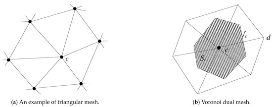
Figure 1.
Definitions of the employed computational mesh. Some notation is introduced and clarified in the text.
Both the action density field N and the transport velocity field are discretized at the vertices of the mesh. They are denoted by and , respectively, with c an index enumerating primal vertices. Once the primal mesh has been defined, a dual mesh must be chosen. Herein, we employ the Delaunay mesh and its dual, the Voronoi tessellation. This is shown in Figure 1b where index c enumerates dual cells. Note that such primal and dual meshes are mutually orthogonal.
We are now in a position to derive a topology-preserving discretization of Equation (6a) using discrete forms. Since action densities are essentially point values, they are referred to as discrete 0-forms, denoted by . Furthermore, we introduce the discrete 2-form representing the cell integrated energy density as follows:
where the integral is over dual cell c (cf. Figure 1b). Lastly, the integral of flux over dual face is given by:
with the outward pointing normal vector to the dual face. This integral quantity is designated as the discrete 1-form and is naturally thought of as the vector component that is normal to the faces of the dual cell.
The exact discretization of Equation (6a) is then given by:
with the discrete exterior derivative, d, acting on the discrete 1-form and yielding a discrete 2-form, which is effectively a divergence of the flux. This operator behaves in all respects like its continuous counterpart implying no loss of physical information during the discretization process.
For each dual cell there is exactly one discrete equation while currently the discrete unknowns are the cell integrated energy density and the face integrated flux . The system of discrete equations becomes closed once these discrete unknowns are related to the primary unknowns at each vertex with the help of the constitutive equations.
First, a discrete relationship between the area integral of energy density in the dual cells and the action density at the primal vertices must be established. Using Equation (6c) and assuming the density of water (discrete 2-form) is constant, a first order approximation yields:
with the size of dual cell c. This numerical approximation is not critical as is usually constant. (If varies in space then it is located at the circumcentre of primal cells and is piecewise uniform within each cell.) In terms of discrete forms, such an approximation is performed by the discrete Hodge star operator that transfers a primal value to a dual value, as follows:
Within the framework of discrete calculus [23], the transformation of flux constitutive Equation (6b) into discrete forms is the following:
implying that the discrete interior product of the discrete 2-form and vector field generates a discrete 1-form. Yet, we will show that most of the numerical errors enter the finite volume method due to this particular reconstruction.
To link the dual mesh to the primal mesh we first consider the discrete 1-form of the velocity vector on the primal mesh. Referring to Figure 1b, this vector is integrated along the edge (or face when viewed in 2D) connecting two vertices c and d, as follows:
Subsequently, this tangential velocity 1-form is used to achieve the primal discrete 1-form with the wedge product specifying the multiplication of a vector with a scalar. Since this result is tangential to the primal edge it can be used to approximate the dual wave action flux 1-form as:
We now elaborate on the obtained discrete formulations to construct the vertex-centered upwind finite volume scheme. In this regard, the discrete forms are considered as piecewise constant over their own mesh objects. Furthermore, for all elaborations below refer to Figure 1b.
First, the line integral of velocity along edge is calculated by means of the standard trapezoidal rule, as follows:
with as the unit tangent vector in the direction of edge and is the edge length. The tangential velocity 1-form is then used to determine the upwind value of wave action with respect to the intersection of the primal edge and the dual face. Accordingly, the discrete form is evaluated as if , otherwise its value is .
Next, to obtain an approximation for the discrete 1-form on dual face , a discrete Hodge star operator is applied. Since the primal edge is perpendicular to the dual face it is calculated as the ratio between the length of the dual face, denoted by , and the length of the primal edge , multiplied by . (Recall that if space varying densities are located in dual vertices then an average of two endpoints of the dual face is taken.) Let denote the discrete counterpart of the face integrated wave action flux on dual face f. Then on dual face it becomes:
This is the simplest first order upwind approximation, which is adequate for the purpose of this study. This type of flux approximation is one of the most commonly used practices in the finite volume framework by which the distinct variables on dual faces are interpolated between nodal values [29]. The associated structured grid variant for the action balance equation has been proposed in, e.g., [34,35]. It should be noted that the treated approximation becomes less accurate when the mesh orthogonality is violated. Extension to non-orthogonal meshes requires a more involved interpolation.
Substitution of approximate constitutive Equations (8) and (10) into topological Equation (7) provides a semidiscrete equation for the wave action density at each vertex c:
with the sum taken over all the faces f of the dual cell. The resulting discrete equation is consistent with transport Equation (5). This scheme for unstructured meshes is the same as the first order vertex-centered upwind finite volume scheme described in [36].
Finally, the first order implicit Euler method is adopted for time discretization, since the action balance equation is known to be rather stiff [39]. Moreover, this method is suitable for steady-state simulations.
In this work we will show that the obtained flux scheme (10) is suboptimal in the sense that the shoaling of the waves near shore is only modeled approximately. This is the key contribution of the current paper. The next section will further elaborate on this.
3.4. Mimetic Flux Approximation
Like many of the material constitutive laws the flux constitutive relation (6b) is local in the sense that the medium is not uniform throughout the space. The bathymetry and, in turn, the wave group velocity can change rapidly, especially in the shallow water regime. Along with the coarse meshes, variations in quantities and N tend to be far stronger than changes in the wave action flux across the dual cells. The application of flux approximation (10) then becomes problematic due to separate treatment of these variables.
In the present study, the approximate Riemann solver of Roe [40] is selected for its ability to preserve flux across discontinuities due to the abrupt transitions in bed topography. Referring to Figure 1b, let discrete 1-form be the integration of the wave action flux along edge :
Consequently,
The approximation of tangential flux 1-form involves the computation of the Roe flux , as follows:
with the characteristic speed and is computed from evaluating the flux Jacobian, such that:
Finally, the discrete Hodge star turns the discrete 1-form on primal edge into the discrete 1-form on dual face , as follows:
This flux approximation can capture exactly a steady discontinuity at the dual cell faces, and can thus be regarded as mimetic. We will show in Section 4 that this leads to a physically consistent wave action transport in case of shoaling, which is another major contribution of this paper.
3.5. Discretization Based on Discrete 0-Form
Since the wave action density is naturally referred to as the points in geographical space, it is principally not a conserved quantity. Instead, transport Equation (4) is rewritten in a conservation form such that a physically suitable conserved quantity can be identified. To this end, we consider a three-dimensional space-time domain and designate as a space-time divergence operator, that is, . Equation (4) is then recast as:
where is the three-dimensional flux and is thus the primary unknown. So Equation (13) describes the local conservation of this flux in space-time; vector field is solenoidal. Its immediate physical implication is wave shoaling: The net flux of action along its wave ray is conserved [41].
We proceed with the discretization. We first consider a space-time slab mesh consisting of three-dimensional triangular prisms, see Figure 2a.
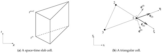
Figure 2.
Local computational cell. Definitions of quantities and notations are provided in the text.
The bottom and top of each prism are the triangular cells at time levels and , respectively. Furthermore, the prism has three rectangular lateral faces. The discretization of Equation (13) is associated with each of these prisms acting as control volumes. In terms of discrete forms it is then given by:
where discrete 2-form is the integrated wave action flux on the prism surface, that is, with the outward-pointing normal to surface (note that dimension n = 3). This is a topological equation that produces an exact discrete 3-form from the prism surface discrete 2-form values; the summation of all the face values on the prism is zero.
Equation (14) is discrete but not closed. Approximations must be invoked to relate the surface integrals to the nodal values of wave action. This is largely an interpolation issue which actually dictates the numerical accuracy. Although many low and high order schemes can be constructed we briefly discuss an approach similar to the one proposed in [33]. In this approach all the necessary interpolations occur within a triangular prism, resulting in a low order method with a compact stencil. In addition, no dual meshes are involved and the method does not require grids to be of a Delaunay type. It should be noted that similar schemes for structured grids are presented in [30,31,32].
Let us consider a triangular cell Δ123 as depicted in Figure 2b for the purpose of actual implementation. Depending on the time integration, this 2D cell corresponds to either the bottom face or the top face of the prism, or in between those faces. The discrete solution at vertices 1, 2, and 3 are denoted by , , and , respectively. The aim is to find an update of wave action in vertex 1. Let an incident wave ray pass through this vertex. If an action flux moves along this ray within the cell from an upstream location to the considered vertex positioned downstream, then the state in vertex 1 is determined solely by the state in the upwind vertices 2 and 3 on the opposite edge.
First, a coordinate mapping from the computational domain to the physical domain is applied. Here are local coordinates and are space-time coordinates. The covariant base vectors in three dimensions are calculated in vertex 1 as follows:
with the position vector of vertex i (the third coordinate is irrelevant and is thus set at zero) and as the time step. Note that the local mapping is chosen such that for , and 3. Since the contravariant base vectors are orthogonal to the covariant base vectors, they are found to be:
where is the Jacobian of the mapping and is expressed by:
representing the volume of the prism under consideration.
Next, exact discretization of Equation (13) is obtained by integration over the triangular prism, in the following way:
where summation convention is applied to Greek indices and,
is the wave action flux component normal to the surface of constant . It should be noted that geometrical quantity is continuous at cell face constant. See [10,11,12] for details.
To complete the discretization, we choose the implicit Euler scheme for the temporal discretization, as time accuracy is not critical to arriving at the steady-state solution. Furthermore, referring to Figure 2b, the two-dimensional covariant and contravariant base vectors, and , respectively, are computed according to:
with the position vector of vertex i, and,
Lastly, the intersection point of the wave ray with velocity through vertex 1 and the opposite edge 23 of triangle Δ123 is located if and . Under these conditions and using one-sided differences, discretization (15) is approximated as follows:
where and are the wave action at time levels and , respectively. This equation is rewritten as:
and is similar to the first order upwind finite difference scheme as presented in, e.g., [32,33,36].
4. Results
In the next two sections, the following numerical schemes are examined for steady-state swell propagation in the nearshore without ambient currents.
- FDM-flux: the flux-conservative upwind finite difference scheme (16);
In [36], the first two schemes are subjected to a convergence test in order to evaluate their spatial accuracy. Scheme FDM-flux shows a higher accuracy over scheme FVM-trad while the latter exhibits a loss of spatial accuracy when the propagation velocity in geographical space is not smooth. This is usually due to jumps in the (sometimes poorly resolved) bathymetry.
The numerical simulations to be presented to employ realistic bathymetric changes. The actual wave processes are wave shoaling and depth-induced refraction and govern the distribution of the variance density with , and the direction of swell propagation [38]. However, since a single swell component is treated, the variance density is computed instead. The governing equation is given by:
with the rate of change of the wave direction along a wave ray due to refraction. The propagation velocity reads while the group velocity is calculated using Equation (2).
The refraction term is approximated with a sufficient directional resolution such that the associated error is significantly smaller than the spatial discretization and interpolation errors. In this respect, the directional space is a closed circular domain while it is divided into sectors with a constant size of , and is the same in all vertices. Further details can be found in [39].
Finally, time stepping is repeated until a stationary solution is obtained. The time derivative performs as a false transient with the pseudo time step and n the iteration counter. This pseudo time step controls the rate of convergence of the iteration process and has proven to be very helpful, especially in solving stiff equations [39].
4.1. Submerged Shoals in Shallow Water
We investigate the performance of the three discussed methods in the presence of two submerged shoals in shallow water, as shown in Figure 3.

Figure 3.
A part of the square domain with bathymetry (in m) of the submerged shoals case as interpolated to the unstructured triangular mesh.
This synthetic test case has also been verified in [36]. The test domain spans 10 km × 10 km and contains two crescent-shaped shoals, the largest spanning 2 km and the smallest about 1 km. The bathymetric depth is 20 m but slopes upward to 1.5 m at the top of the largest shoal and upward to 3.5 m at the top of the smallest shoal. The unstructured mesh consists of 1504 triangles with the grid size varying in between 100 and 400 m, providing an economical representation of the bathymetric features. At the south boundary, a monochromatic, long-crested swell wave is imposed with a height of 1 m, a period of 15 s, and a direction pointing northward.
Before evaluating the schemes in the test case involving both shoaling and refraction, they are evaluated first in a case in which waves shoal over the sloping beds. This test case was set up with the objective to inspect energy flux conservation. In this context, Equation (17) with is considered as a ray equation for wave packets propagating along parallel wave rays by which the net flux of energy is constant. By virtue of this physical principle, the (dimensionless) shoaling coefficient proportional to can be tested [38].
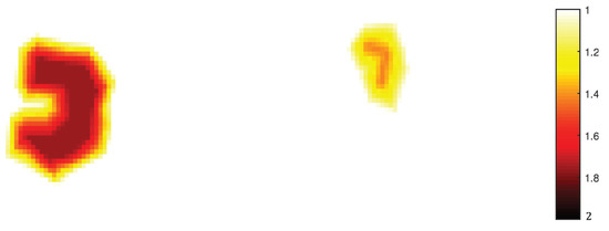
Figure 4.
Spatial distribution of shoaling coefficient obtained with scheme FDM-flux.
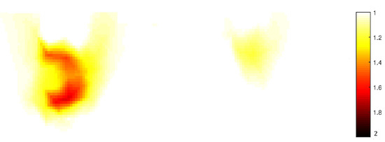
Figure 5.
Spatial distribution of shoaling coefficient obtained with scheme FVM-trad.
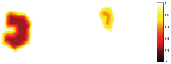
Figure 6.
Spatial distribution of shoaling coefficient obtained with scheme FVM-Roe.
Method FDM-flux displays correctly the spatial distribution of the shoaling coefficient across the shoals as it changes locally with the water depth (compare Figure 4 to Figure 3).
In contrast, the result of scheme FVM-trad is clearly non-physical as displayed in Figure 5. The spatial distribution of wave energy throughout the domain is erroneous, owing to Equation (9) while the velocity field is irregular. However, the solution improves substantially when the mimetic flux approximation of Roe, that is, Equation (12), is selected which leads to correct wave shoaling over rising bottoms around the shoals (cf. Figure 6).
Note that both schemes FDM-flux and FVM-Roe yield identical results.
The next simulations are the ones with depth refraction included. In this regard, we consider the total variance of the surface elevation across the domain,
and the mean wave direction,
The results obtained with the FDM-flux method is depicted in Figure 7.
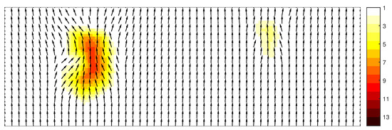
Figure 7.
Spatial distribution of total variance (in m) and vector plot of mean wave direction obtained with scheme FDM-flux.
The refracted waves at shallower depths are clearly evidenced. There is a convergence of energy when the swell approaches the shoal and a divergence of energy when it leaves the shoal. This is consistent with the Snel’s law [38]. Accordingly, the wave energy increases on top of the shoal.
Figure 8 shows the results produced by the FVM-trad scheme. Wave turning is greatly exaggerated at the large shoal.
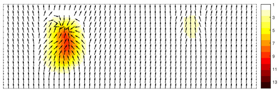
Figure 8.
Spatial distribution of total variance (in m) and vector plot of mean wave direction obtained with scheme FVM-trad.
This non-physical response is caused by the lack of flux conservation in geographical space. This negatively affects wave shoaling, and in turn, it inevitably impacts the refraction (cf. Equation (17)). Yet, when scheme FVM-Roe is employed, this erratic behavior disappears and the solution is qualitatively similar to that of FDM-flux, see Figure 9.
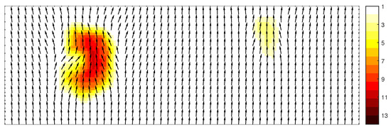
Figure 9.
Spatial distribution of total variance (in m) and vector plot of mean wave direction obtained with scheme FVM-Roe.
4.2. The Haringvliet Bay Case
The Haringvliet is a branch of the Rhine estuary in the south-west of the Netherlands. The shallow bay that penetrates into the shoreline is somewhat protected from the North Sea by a shallow shoal called the Hinderplaat where steep bathymetric gradients are present. The depth variations are the main cause of the shoaling and turning of the swells approaching the submerged shoal. In this context, the aim of the present test is to illustrate the comparative performance of the three discussed schemes in terms of conservation properties. In order to demonstrate errors due to a lack of flux conservation that have a significant effect on the swell height, wave processes of generation, redistribution, and dissipation are ignored for this test case.
We employ a triangular (Delaunay) mesh where the size of the cells is proportional to the water depth, see Figure 10.
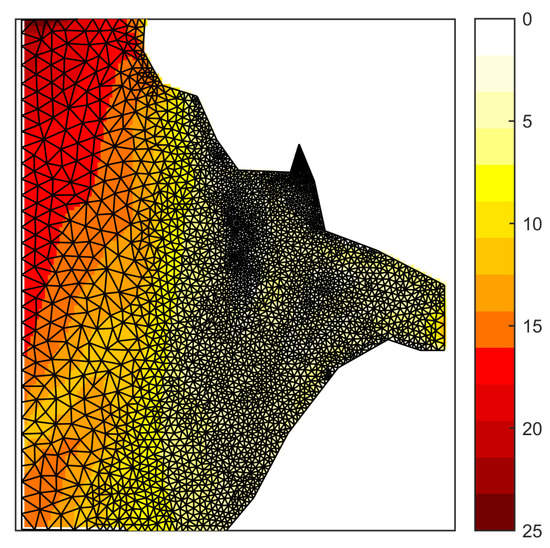
Figure 10.
Bathymetry (m) of the Haringvliet Bay case projected on the triangular mesh.
The minimum size of the cells is to be found in the area around the Hinderplaat. The mesh spacings are sufficient to resolve the refraction process in this region. There are approximately 6000 cells in total. An incoming swell propagating in the direction to the east is specified at the west boundary with a height of 0.4 m and a period of 15 s. In addition, the mean water level is raised by 0.6 m so that the deactivation of the depth-induced breaking is justified [38].
Figure 11 depicts the computed spatial distribution of increased wave heights, with respect to the incident swell around the shoal obtained from the numerical schemes (panels b–d).
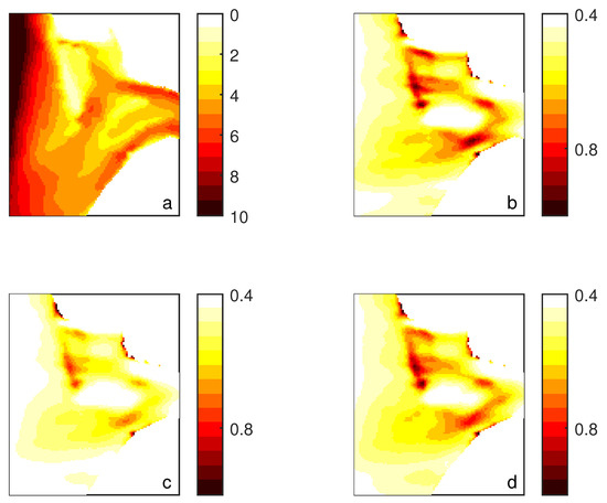
Figure 11.
Spatial distribution of (a) water depth (m) around the shoal Hinderplaat and wave height (m) obtained with scheme (b) FDM-flux, (c) FVM-trad, and (d) FVM-Roe.
The water depth in the same area is also provided for a proper interpretation (panel a). It can be observed that the largest waves correlate strongly with the shallowest depths of the bay. Furthermore, the figure reveals that the result of scheme FVM-trad (Figure 11c) clearly differs from the other schemes (Figure 11b,d) while the solution of scheme FVM-Roe is very similar to the solution of scheme FDM-flux. Yet, the results obtained from the two last mentioned mimetic schemes are expected to be more in line with the physics. On that same note, the lack of energy flux conservation of the traditional finite volume scheme underestimates the amount of wave energy fairly. This deficit has been previously observed in the former test case and is expected to limit physical accuracy.
5. Conclusions
In this work, a discrete calculus approach to develop physically consistent discretizations for the action balance equation was presented. The key was to make a clear separation between the exact discretization of differential operators and the approximation of constitutive relations. In doing so, the discretization methods as outlined in [36] were reconstructed in an effort to point out the presence or the lack of wave action flux conservation. The preference of the upwind finite difference scheme compared with the vertex-centred upwind finite volume scheme in physical accuracy was plainly demonstrated. As the latter scheme suffered from a lack of flux conservation, an improved flux approximation was proposed, based on Roe’s numerical flux scheme which preserves the wave action flux exactly at the discrete level.
The numerical examples herein illustrated that the treated low order mimetic schemes guaranteed the state of zero divergence of wave action flux field to be satisfied up to machine accuracy. Their mimetic nature stands out in the ability to exactly simulate the shoaling of the swell propagating over variable depth, and consequently the interplay between refraction and shoaling.
The above conclusions are specific to the transformation of swell waves over seafloor topography. Indeed, the local changes of the swell under depth-limited conditions require a greater degree of numerical accuracy, while the level of prediction accuracy of the wind-sea spectrum commonly relies on the semi-empirical nature of the theory describing the physical processes involved (e.g., generation by wind, dissipation due to white capping), given that the bathymetric features and wind forcing were accurately resolved. At any rate, the numerical performances of the studied methods in this paper clearly demonstrate the need for a physically consistent discretization to enhance the correctness of the numerical solution to the action balance equation. Such a discretization should therefore be a prerequisite for a proper assessment of spectral wave models.
Funding
This work received no funding.
Conflicts of Interest
The author declares no conflict of interest.
References
- Richtmyer, R.D.; Morton, K.W. Difference Methods for Initial Value Problems; John Wiley and Sons: New York, NY, USA, 1967. [Google Scholar]
- Mattiussi, C. An analysis of finite volume, finite element, and finite difference methods using some concepts from algebraic topology. J. Comput. Phys. 1997, 133, 289–309. [Google Scholar] [CrossRef]
- Tonti, E. Why starting from differential equations for computational physics? J. Comput. Phys. 2014, 257, 1260–1290. [Google Scholar] [CrossRef]
- Ferretti, E. The algebraic formulation: Why and how to use it. Curved Layer. Struct. 2015, 2, 106–149. [Google Scholar] [CrossRef]
- Morinishi, Y.; Lund, T.S.; Vasilyev, O.V.; Moin, P. Fully conservative higher order finite difference schemes for incompressible flow. J. Comput. Phys. 1998, 143, 90–124. [Google Scholar] [CrossRef]
- Verstappen, R.W.C.P.; Veldman, A.E.P. Symmetry-preserving discretization of turbulent flow. J. Comput. Phys. 2003, 187, 343–368. [Google Scholar] [CrossRef]
- van’t Hof, B.; Veldman, A.E.P. Mass, momentum and energy conserving (MaMEC) discretizations on general grids for the compressible Euler and shallow water equations. J. Comput. Phys. 2012, 231, 4723–4744. [Google Scholar] [CrossRef]
- Harlow, F.H.; Welch, J.E. Numerical calculation of time-dependent viscous incompressible flow of fluid with free surface. Phys. Fluids 1965, 8, 2182–2189. [Google Scholar] [CrossRef]
- Arakawa, A.; Lamb, V.R. A potential enstrophy and energy conserving scheme for the shallow water equations. Mon. Weather Rev. 1981, 109, 18–36. [Google Scholar] [CrossRef]
- Wesseling, P.; Segal, A.; van Kan, J.; Oosterlee, C.; Kassels, C. Finite volume discretization of the incompressible Navier-Stokes equations in general coordinates on staggered grids. Comput. Fluid Dyn. J. 1992, 1, 27–33. [Google Scholar]
- van Beek, P.; van Nooyen, R.; Wesseling, P. Accurate discretization of gradients on non-uniform curvilinear staggered grids. J. Comput. Phys. 1995, 117, 364–367. [Google Scholar] [CrossRef]
- Zijlema, M.; Segal, A.; Wesseling, P. Finite volume computation of incompressible turbulent flows in general co-ordinates on staggered grids. Int. J. Numer. Meth. Fluids 1995, 20, 621–640. [Google Scholar] [CrossRef]
- Hall, C.A.; Cavendish, J.C.; Frey, W.H. The dual variable method for solving fluid flow difference equations on Delaunay triangulations. Comput. Fluids 1991, 20, 145–164. [Google Scholar] [CrossRef]
- Nicolaides, R.A. Direct discretization of planar div-curl problems. SIAM J. Numer. Anal. 1992, 29, 32–56. [Google Scholar] [CrossRef]
- Perot, B. Conservation properties of unstructured staggered mesh schemes. J. Comput. Phys. 2000, 159, 58–89. [Google Scholar] [CrossRef]
- Stuhne, G.R.; Peltier, W.R. A robust unstructured grid discretization for 3-dimensional hydrostatic flows in spherical geometry: A new numerical structure for ocean general circulation modeling. J. Comput. Phys. 2006, 213, 704–729. [Google Scholar] [CrossRef]
- Thuburn, J.; Cotter, C.J. A framework for mimetic discretization of the rotating shallow-water equations on arbitrary polygonal grids. SIAM J. Sci. Comput. 2012, 34, B203–B225. [Google Scholar] [CrossRef]
- Danilov, S. Ocean modeling on unstructured meshes. Ocean Model. 2013, 69, 195–210. [Google Scholar] [CrossRef]
- Korn, P. Formulation of an unstructured grid model for global ocean dynamics. J. Comput. Phys. 2017, 339, 525–552. [Google Scholar] [CrossRef]
- Arakawa, A. Computational design for long-term numerical integration of the equations of fluid motion: Two-dimensional incompressible flow. Part I. J. Comput. Phys. 1966, 1, 119–143. [Google Scholar] [CrossRef]
- Lipnikov, K.; Manzini, G.; Shashkov, M. Mimetic finite difference method. J. Comput. Phys. 2014, 257, 1163–1227. [Google Scholar] [CrossRef]
- Palha, A.; Gerritsma, M. A mass, energy, enstrophy and vorticity conserving (MEEVC) mimetic spectral element discretization for the 2D incompressible Navier-Stokes equations. J. Comput. Phys. 2017, 328, 200–220. [Google Scholar] [CrossRef]
- Desbrun, M.; Hirani, A.N.; Leok, M.; Marsden, J.E. Discrete exterior calculus. arXiv 2005, arXiv:math/0508341v2. [Google Scholar]
- Bochev, P.B.; Hyman, J.M. Principles of mimetic discretizations of differential operators. In Compatible Spatial Discretizations. The IMA Volumes in Mathematics and Its Applications; Arnold, D.N., Bochev, P.B., Lehoucq, R.B., Nicolaides, R.A., Shashkov, M., Eds.; Springer: New York, NY, USA, 2006; Volume 142, pp. 89–120. [Google Scholar]
- Perot, J.B.; Zusi, C.J. Differential forms for scientists and engineers. J. Comput. Phys. 2014, 257, 1373–1393. [Google Scholar] [CrossRef]
- Grady, L.J.; Polimeni, J.R. Discrete Calculus-Applied Analysis on Graphs for Computational Science; Springer: London, UK, 2010. [Google Scholar]
- Steinberg, S. The accuracy of numerical models for continuum problems. In Error Control and Adaptivity in Scientific Computing; Bulgak, H., Zenger, C., Eds.; Springer: Dordrecht, The Netherlands, 1999; pp. 299–323. [Google Scholar]
- Perot, J.B.; Subramanian, V. Discrete calculus methods for diffusion. J. Comput. Phys. 2007, 224, 59–81. [Google Scholar] [CrossRef]
- Ferziger, J.H.; Perić, M. Computational Methods for Fluid Dynamics, 3rd ed.; Springer: Berlin, Germany, 2002. [Google Scholar]
- The WAMDI Group. The WAM model-A third generation ocean wave prediction model. J. Phys. Oceanogr. 1988, 18, 1775–1810. [Google Scholar] [CrossRef]
- Tolman, H.L. A third-generation model for wind waves on slowly varying, unsteady and inhomogeneous depths and currents. J. Phys. Oceanogr. 1991, 21, 782–797. [Google Scholar] [CrossRef]
- Booij, N.; Ris, R.C.; Holthuijsen, L.H. A third-generation wave model for coastal regions 1. Model description and validation. J. Geoph. Res. 1999, 104, 7649–7666. [Google Scholar] [CrossRef]
- Zijlema, M. Computation of wind-wave spectra in coastal waters with SWAN on unstructured grids. Coast. Eng. 2010, 57, 267–277. [Google Scholar] [CrossRef]
- Hubbert, K.P.; Wolf, J. Numerical investigation of depth and current refraction of waves. J. Geoph. Res. 1991, 96, 2737–2748. [Google Scholar] [CrossRef]
- Janssen, P.A.E.M. Progress in ocean wave forecasting. J. Comput. Phys. 2008, 227, 3572–3594. [Google Scholar] [CrossRef]
- Zijlema, M. Accuracy aspects of conventional discretization methods for scalar transport with nonzero divergence velocity field arising from the energy balance equation. Int. J. Numer. Meth. Fluids 2021. [Google Scholar] [CrossRef]
- Komen, G.J.; Cavaleri, L.; Donelan, M.; Hasselmann, K.; Hasselmann, S.; Janssen, P.A.E.M. Dynamics and Modelling of Ocean Waves; Cambridge University Press: Cambridge, UK, 1994. [Google Scholar]
- Holthuijsen, L.H. Waves in Oceanic and Coastal Waters; Cambridge University Press: Cambridge, UK, 2007. [Google Scholar]
- Zijlema, M.; Van der Westhuysen, A.J. On convergence behaviour and numerical accuracy in stationary SWAN simulation of nearshore wind wave spectra. Coast. Eng. 2005, 52, 237–256. [Google Scholar] [CrossRef]
- Roe, P.L. Approximate Riemann solvers, parameter vectors and difference schemes. J. Comput. Phys. 1981, 43, 357–372. [Google Scholar] [CrossRef]
- Whitham, G.B. Linear and Nonlinear Waves; John Wiley and Sons: New York, NY, USA, 1974. [Google Scholar]


Publisher’s Note: MDPI stays neutral with regard to jurisdictional claims in published maps and institutional affiliations. |
© 2021 by the author. Licensee MDPI, Basel, Switzerland. This article is an open access article distributed under the terms and conditions of the Creative Commons Attribution (CC BY) license (http://creativecommons.org/licenses/by/4.0/).