1. Introduction
Climatic test chambers are widely used in research and product development in industrial applications to conduct tests on manufactured samples, specimens, or components under controlled environmental conditions. Despite the increasing interest in the use of climatic chambers in various research fields and industries, only a few valid scientific works have focused on the analysis of their thermofluidic performance, either experimentally or numerically. Liang et al. [
1] provided a mathematical model to investigate the transient thermal performance of a full-sized vehicle climate chamber and suggested solutions to improve heating and cooling rates. Dostál et al. [
2] presented a control algorithm using a predictive control method model for a climatic chamber, and García-Contreras et al. [
3] proposed a theoretical and experimental methodology to obtain the thermal loads for a climatic vehicle test chamber. The performance of a temperature and humidity chamber was evaluated by Mensah et al. [
4] experimentally. In another study, three-dimensional CFD thermofluidic modelling was carried out for a test chamber by Candanedo et al. [
5], and the results were validated experimentally. A numerical and experimental study was performed by Lecoq et al. [
6] on the evaporation rate in a cold chamber, and in a recent study, the application of CFD modelling to predict the air circulation in an evaporator of a large-scale heat pump was studied by Rogié et al. [
7] using Ansys Fluent.
Yuan Liu et al. [
8] were able to obtain good agreement between theoretical and numerical simulations, which coupled heat and moisture, but the data were not verified experimentally. In another study, Vojkuvkova et al. [
9] used CFD modelling to investigate the condensation and freezing of water vapour in a mixing chamber. Their results showed that the most condensation occurs on the upper parts of walls. In another study, CFD modelling was applied by Shojaee Nasirabadi et al. [
10] to simulate the moisture transfer throughout an electronic enclosure. The results show that the local environment inside the enclosure responds faster to the temperature changes than it does to the relative humidity variations. They also found good agreement between the numerical simulation results and experimental results from the literature.
This work, however, aims to fill a gap in the climatic chamber equipment modelling, which typically is only concerned with modelling the temperature and velocity fields. It provides a 3-D thermofluidic CFD model to analyse the fluid flow, heat, and mass transfer behaviour of a new climatic chamber prototype designed by the industrial company Aralab, with the collaboration of the Itecons research centre. This model is based on a 300 L inner volume chamber that was numerically and experimentally studied by Silva et al. [
11].
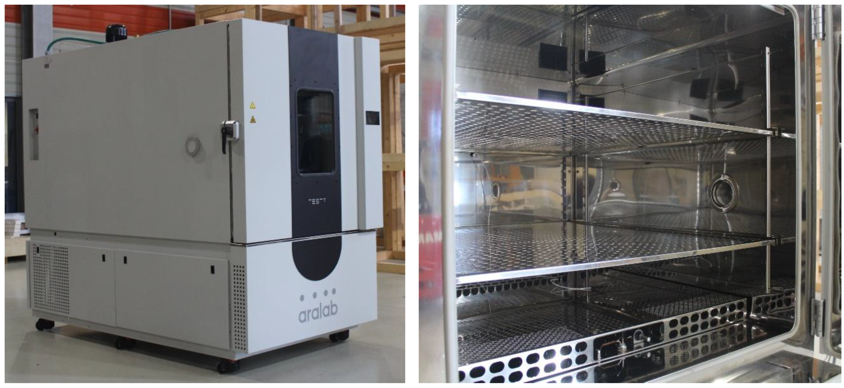
This new climatic chamber has an inner box with 1200 L capacity, which is used to keep test specimens, and a smaller box in which the evaporator, electric heater resistance, and ventilation equipment is located (
Figure 1). The technical information for the chamber is presented in
Table 1.
Compared with the previous model of this equipment and others readily available in the market, this new climatic chamber was equipped with variable compressors and variable ventilators, an optimised reduction of the rock−wool wall insulation thickness was also applied, and an eco-friendly refrigerant was adopted. These changes lead to a reduction in energy consumption and acoustic noise emission. However, they make it critically necessary to study their effect on the homogeneity of the temperature and the relative humidity inside the test chamber throughout its use, and to ascertain the need to modify or create optimised air flow routes.
This paper first describes the 3D CFD model of the climate chamber that was developed using Ansys Fluent to simulate the fluid flow, heat, and mass transfer. Then, the thermofluidic performance of the chamber is presented, based on the simulation results, and the heat loss from the surrounding components of the chamber is calculated to arrive at a fixed internal temperature. Finally, the numerical model was validated using experimental data, comparing the results for fluid flow velocity, temperature, and relative humidity.
2. Geometry
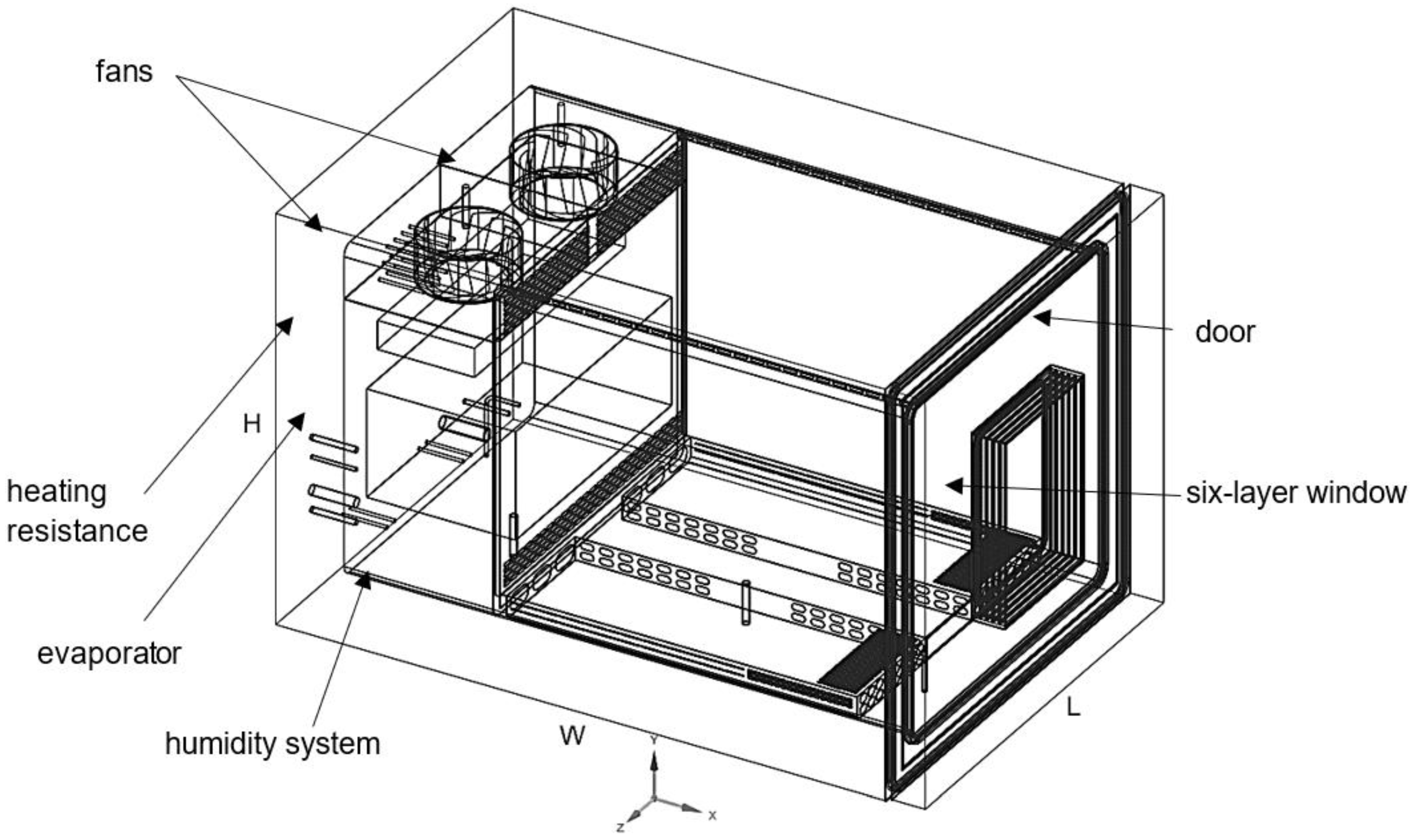
The 3D model of the climatic chamber was developed using the software SolidWorks and Ansys SpaceClaim 19.2. The key components of the chamber that were modelled included the top, bottom, and back perforated grids of the testing box, thermal insulation walls, door component together with a six-layer glass window, evaporator, heat resistances, piping, water storage (humidity system), and two fans. The climatic chamber under study had the following external dimensions: L = 1.25 m, H = 1.24 m, and W = 1.84 m (see
Figure 2).
Additionally, the temperature was controlled using the heating electric resistances and the evaporator located near the fans, and the relative humidity was controlled via a humidity system, which heats up a reservoir of water using an electric resistance or cools down the fluid, leading to condensation of vapour into the reservoir, depending on whether the relative humidity is to be increased or reduced, respectively.
3. Model Setup
3.1. Mesh
The Ansys Fluent finite volume method (FVM) [
12,
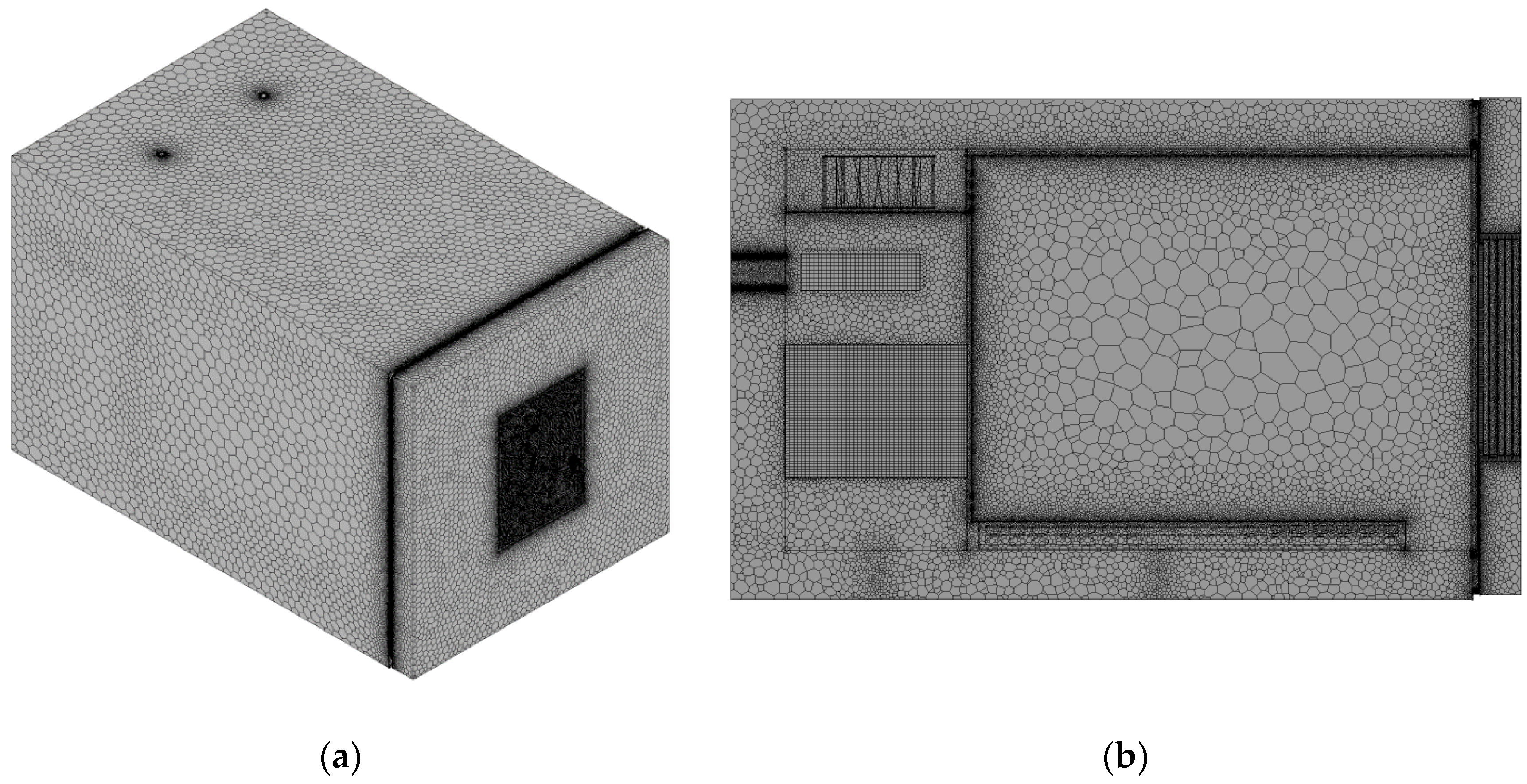
13] was used to solve the fundamental equations governing heat transfer and fluid flow. This was performed using an Ansys Mesher and a nonstructured tetrahedral mesh. In the meshing process, a sweep method was used for meshing the sweepable components. The mesh was then converted into polyhedral elements in Ansys Fluent to increase precision, convergence, and robustness.
Figure 3 illustrates the mesh structure used to model the solid parts and the fluid.
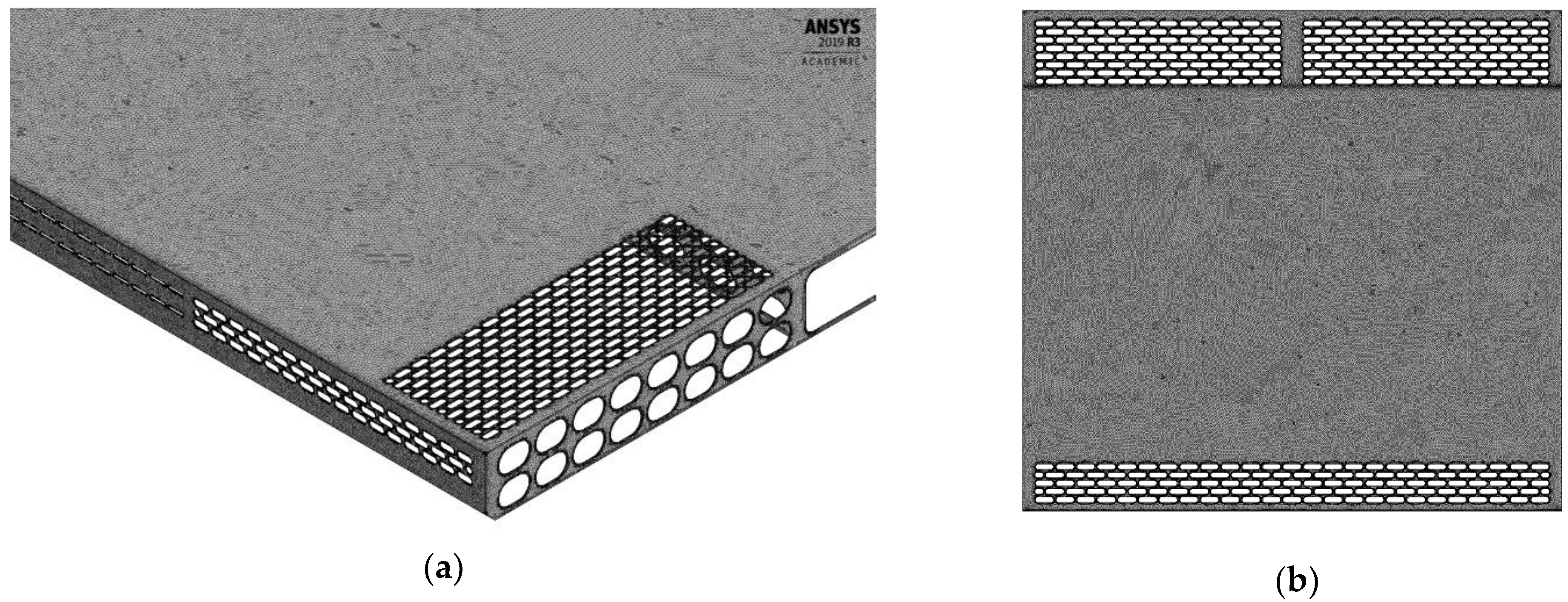
The mesh was refined in the zones that required more accuracy, such as the components with a more detailed geometry (
Figure 4).
The mesh was optimised and partitioned in Ansys Fluent using the Cuthill–McKee inverse method [
14] and METIS algorithm, respectively [
15,
16]. The final number of elements of the model was 33.14 million. The grid independence study was performed to ensure that the solution did not change with further refinement. With this in mind, while the number of elements increased, convergence of the monitored variables was checked. By increasing the number of elements to 48.19 million, the average temperature of the air inside changed by approximately 0.03%, which shows the high degree of independence of the results with respect to the mesh size. To ensure successful computations of the interior turbulent flows of the climatic chamber, mesh generation must be well defined in the regions where the mean flow undergoes rapid changes and the shear layers have large strain rates. By computing the first cells’ height near the wall, based on the average fluid velocity, length scale, viscosity, and density, the target
near the walls of the climatic chamber was achieved by imposing discretised inflation layers on 10 cells with a constant growth rate of 1.2, and the obtained
was equal to 0.98.
In this study, Ansys Fluent was used to solve the mass, momentum, and energy conservation equations for the entire domain using the finite volume method (FVM) [
17]. The fundamental equations of mass, momentum, and energy conservation can be found in Cengel et al. [
18]. The fluid flow was considered to be a turbulent regime in the inlet during nominal operation conditions. Turbulent flow is governed by the Navier–Stokes momentum equations, the continuity equations, and in compressible flow, the energy and state equations. In this study, the turbulent flow was modelled using the Reynolds-averaged Navier–Stokes (RANS) equations and four different turbulent models: k−ω SST, k−ε standard, k−ε RNG, and k−ε realisable. The governing equations can be found in detail in [
14,
19]. Reynolds-averaged Navier–Stokes (RANS) is the most widely used class of turbulence models in applied research due to their fast computation time and excellent convergence characteristics and because they can be used in combination with steady-state simulations [
20]. To investigate the humidity distribution inside the chamber, the species transport model in Ansys Fluent was applied in the steady-state model. A certain amount of the mass fraction of water was introduced into the air circulation, depending on the relative humidity set point. As the main aim of the study is to assess the temperature and humidity distribution in the testing area of the chamber, the phase change due to evaporation and condensation is ignored in this model. The mass diffusion in turbulent flows is computed using the following equation:
where
is the mass diffusion coefficient for species,
is the local mass fraction of species,
is the turbulent viscosity,
is the turbulent Schmidt number, and
is the thermal diffusion coefficient.
Furthermore, the transport of enthalpy due to mass diffusion, which has a significant effect on the enthalpy field, was calculated in Ansys Fluent. More information regarding the species transport model can be found in the Ansys Fluent manual [
17].
3.2. Boundary Conditions
3.2.1. Exterior Wall
The convection heat transferring through the external wall to the air surrounding the equipment can be calculated using Newton’s law of cooling:
where
is the external convection coefficient,
is the area of the wall,
is the surface temperature, and
is the ambient temperature. This value is obtained from the average Nusselt number, which is given by the following correlation:
where
is the thermal conductivity and
is the characteristic length of the geometry, which is equal to the lateral/horizontal size of the lateral/horizontal plate. For plates of various shapes (e.g., rounded corners), this characteristic length can be defined as [
21]:
where
and
are the plate surface area (one side) and perimeter, respectively.
For the horizontal plate, the flow patterns and heat transfer depend strongly on whether the surface is cold or hot and on whether it is facing up or down [
22]. Therefore, the average Nusselt numbers for the top and bottom surfaces are obtained from the following equations. For the upper surface of the hot plate (Equation (4)) and the lower surface of the cold plate (Equation (5)), the average Nusselt numbers are:
and for the lower surface of the hot plate and the upper surface of the cold plate, the average Nusselt number is:
where,
is the Prandtl number and
is the Rayleigh number based on the plate length, which is given by the following equation:
where
is the gravitational acceleration,
represents the fluid thermal expansion,
is the kinematic viscosity, and
is the thermal diffusivity.
For the lateral walls, the average Nusselt number can be calculated from the correlation, which has been recommended by Churchill and Chu [
22] and may be applied over the entire range of
:
For the inclined plates, it was suggested by Rich [
23] that the convection coefficient could be determined from the vertical plate correlation if
is replaced by
in computing the plate Rayleigh number. However, this approach is only satisfactory for the top and bottom surfaces of cold and hot plates, respectively. No recommendations are made for the opposite surfaces. The heat transfer calculations were performed according to an external air temperature of 22 °C.
3.2.2. Radial Fan
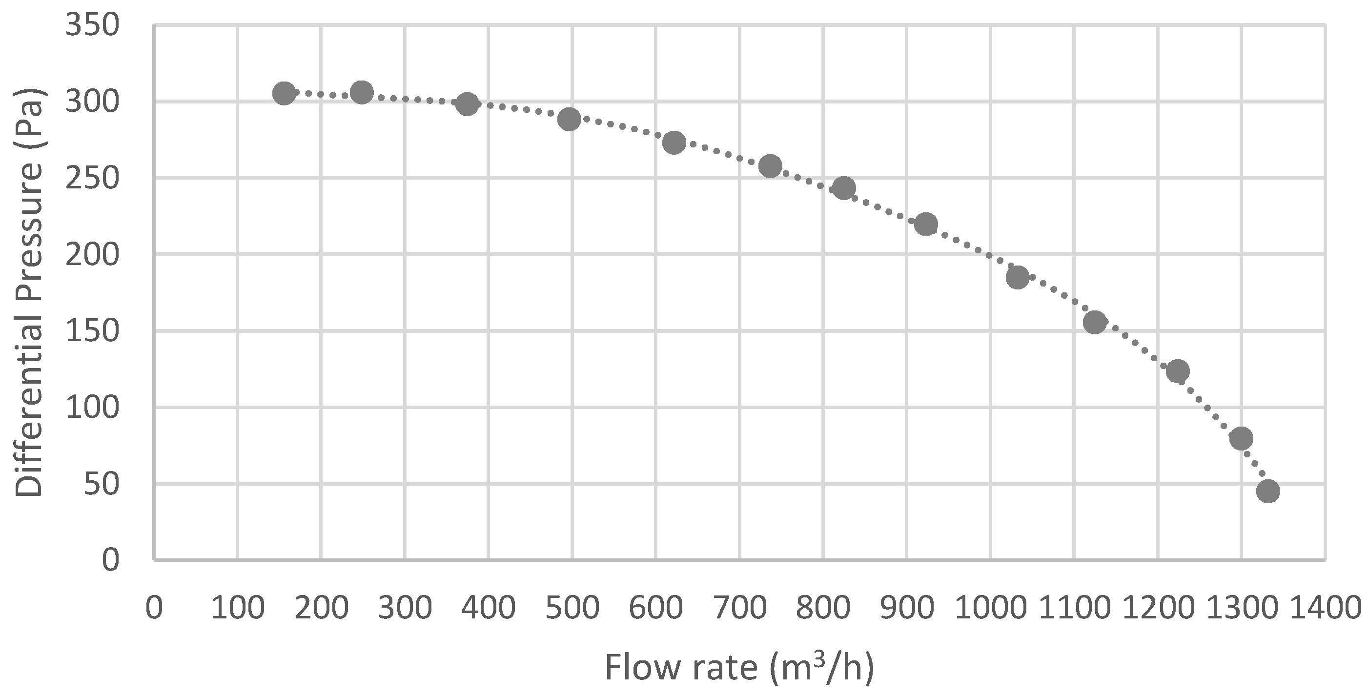
The climatic chamber uses two radial fans with variable speed, which rotate in opposite directions to ensure homogeneous distribution of temperature and moisture inside the chamber. The characteristic curve of the fan is presented in
Figure 5. The diameter of the fan’s rotor is 28 cm with a maximum flow rate of
and a maximum axial velocity of
. The modelling was performed using the internal boundary condition and by introducing the uniform pressure jump variables for both fans, as defined by the manufacturer.
The fan was considered to be adiabatic and with no entropy losses and, therefore, without any viscous dissipation. For simplification, the 3D rotating fans in the CFD model were ignored, and 1D flow through the pressure jump was considered. The pressure differential of the fan in Pascal as a function of the axial average velocity (
) in m/s was obtained as follows:
3.2.3. Electric Resistance
The electrical resistance that supplies thermal energy was modelled as a uniformly distributed heat source in the location of the actual electric resistance in the chamber. The electrical supply of this chamber consists of 6 resistances, each with an electric power of . Therefore, a total thermal power of was considered for the input electrical thermal power of the heat resistance, assuming no heat loss and 100% electrical-to-thermal-conversion efficiency.
3.2.4. Evaporator
The evaporator developed for this chamber was of the tube-fin heat exchanger type. It is important to model the evaporator to consider the pressure loss in the air flow. Modelling the evaporator with all the fins and tubes in Ansys Fluent is complex and inefficient. Hence, the pressure loss in the evaporator was computed and modelled as an anisotropic porous medium [
24]. The pressure loss through the anisotropic porous medium depends on the magnitude of the velocity and is given by the equation:
where,
is the density of the fluid,
is the inertial resistance coefficient, and
is the velocity norm (perpendicular to the inflow). To obtain
in Equation (10), the constant terms of Equation (11) for the core friction in the evaporator were calculated and equalised to
.
where,
is the friction factor,
is the core length, and
is the hydraulic radius. According to the manufacturer, the value of 0.23 was considered for the air-side friction factor. It is important to note that to consider the effects of baffles on the fluid flow, the other pressure loss coefficients in the direction perpendicular to the fins were set to the large values. This provided a
value of 40.35 m
−1, which was used as the simulation input data.
3.3. Material Properties
The air properties were considered to vary with temperature ( in Kelvin). The solids in this study are stainless steel, used in the box structure and pipes; rubber, glass, and copper for heat resistances and evaporator tubes; and rock−wool as the insulation to prevent heat loss from the chamber walls and door.
The air properties, including the density, dynamic viscosity, thermal conductivity, and specific heat, were assumed to vary with the temperature and were obtained from [
11], based on interpolated data from Keenan [
25] and Touloukian [
26], and can be expressed as follows:
The solid material properties are obtained from data provided by the manufacturer, as indicated in
Table 2.
For the thermal insulation, the thermal conductivity was considered to be dependent on the temperature and can be achieved by the equations listed in
Table 2 (where
is the temperature of the insulation in Kelvin).
3.4. Solver
The air behaviour was considered as an incompressible fluid, and a pressure-based solver was used, requiring less memory and allowing for flexibility in the solution procedure. In order to evaluate diffusive fluxes and velocity derivatives, the gradient of solution variables is required. The Green–Gauss cell-based approach was used for this, while the robustness of the SIMPLE algorithm led to it being used for the pressure–velocity coupling. The PRESTO! method was used for calculating cell-face pressure, which is highly recommended for flows involving steep pressure gradients or in strongly curved domains. The first-order upwind method was used for the remaining interpolation arrangements for robustness and easy convergence [
12].
3.5. Convergence
At convergence, as mentioned in the Ansys customer training material, the following should be satisfied:
• The solution no longer changes with subsequent iterations.
• Overall mass, momentum, energy, and scalar balances are achieved.
• All equations (momentum, energy, etc.) are obeyed in all cells to a specified tolerance.
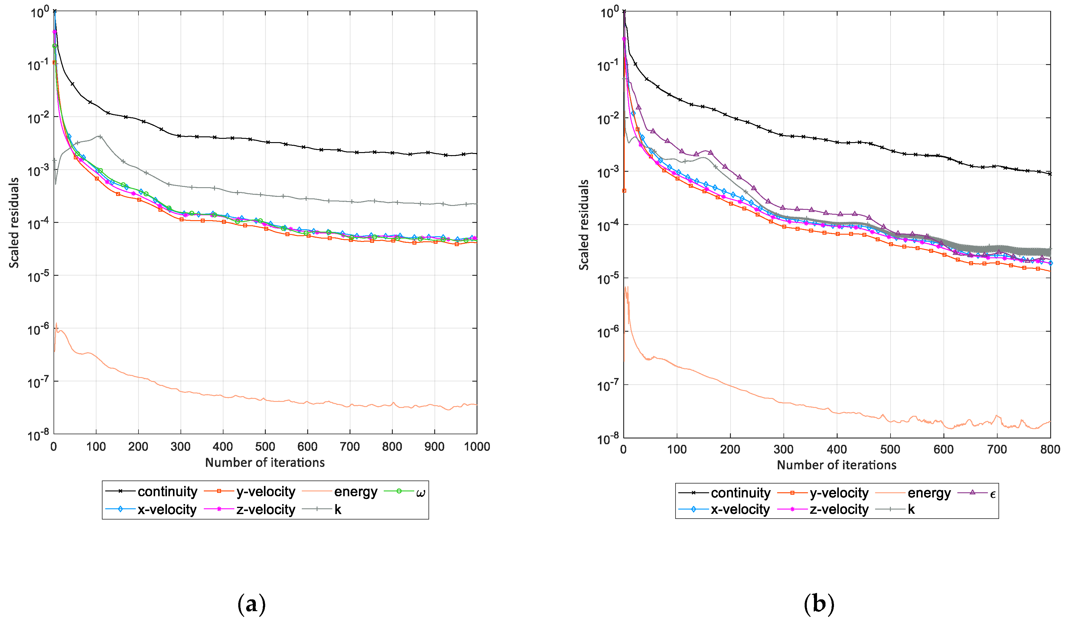
The convergence conditions were monitored for all turbulence models and were found to be adequate.
Figure 6 illustrates the convergence of all scaled residuals associated with the mass, momentum, and energy conservation for the k−ω SST model and k−ε RNG model.
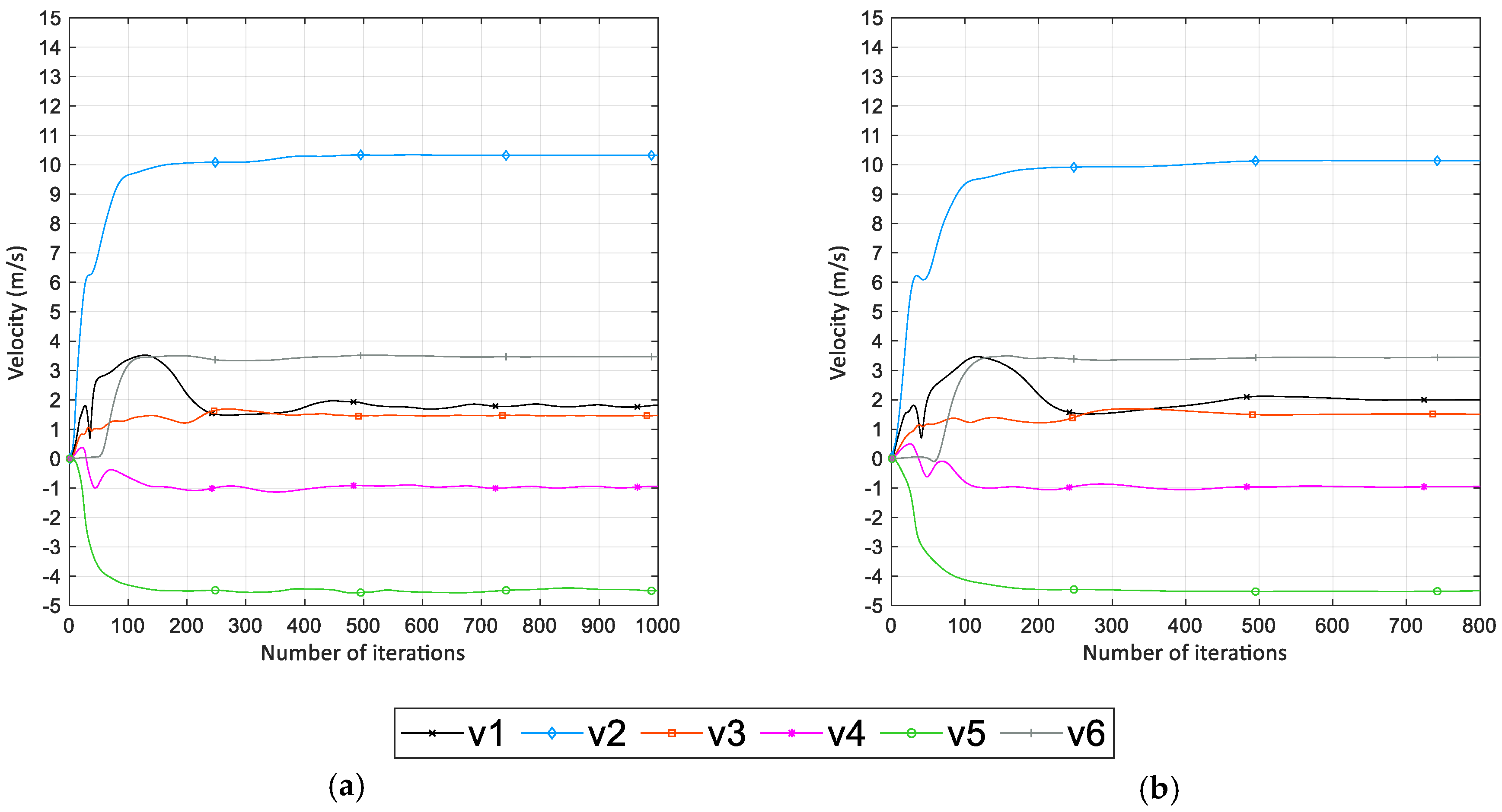
Additionally, three representative local velocities at six points (inside the box) including v1 (−0.13, 1.59, 0), v2 (−0.19, 1.66, 0.23), v3 (0, 1.46, 0.35), v4 (0, 1.4, −0.15), v5 (−0.43, 0.82, 0), and v6 (0.81, 1.46, −0.4) were monitored to ensure convergence (
Figure 7).
4. Experimental Tests
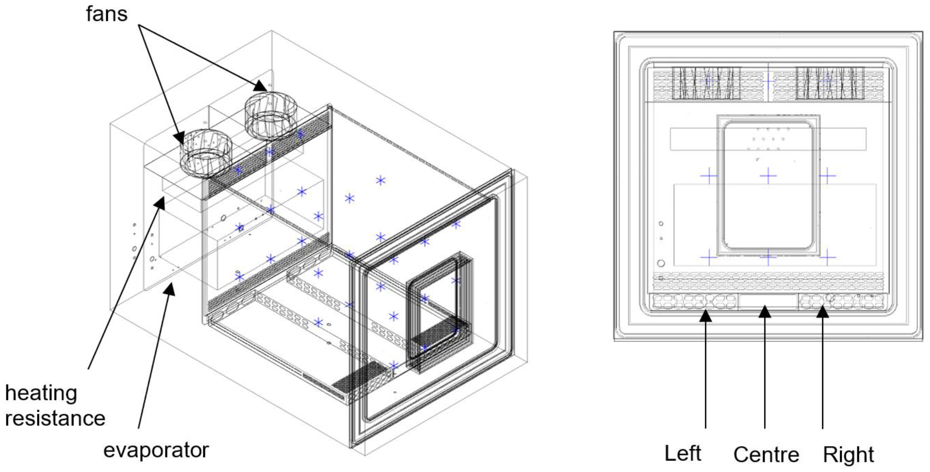
A series of experiments were performed by recording the velocities and temperatures inside the climatic chamber. A unidirectional TA410 anemometer, with an accuracy of ±5%, and a calibrated type-K thermocouple, with an accuracy of ±0.3 °C, were installed to measure the velocity and temperature at 27 points inside the chamber. The positions of the monitoring points are shown in
Figure 8.
At this stage, the set point temperature of the equipment was set to 25 °C and was kept constant during the measurement. The velocity was measured for the three planes, including the left, centre, and right sections, and for three different distances from the door and the ceiling. Nine points were used in each plane.
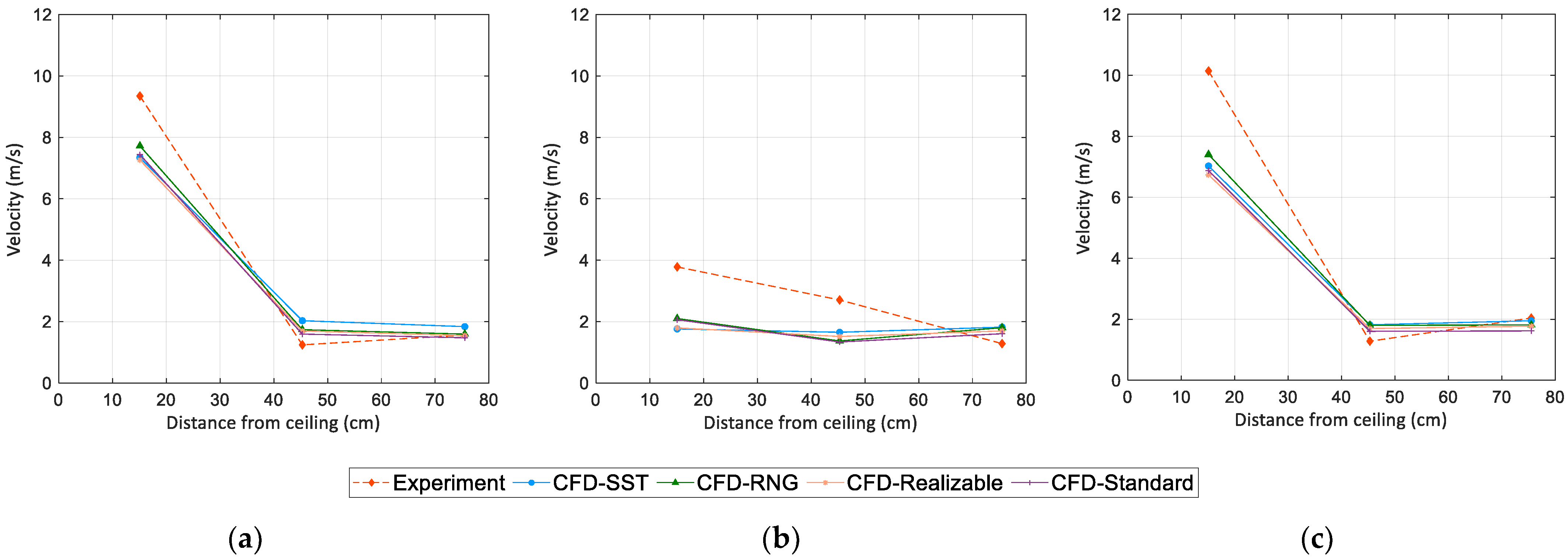
Figure 9 shows a comparison between the average results for each plane obtained from experimental measurements and those obtained from CFD modelling four turbulence models. The largest difference between the experimental and numerical analyses was observed for the velocity field over the top section of the chamber, where the larger velocity gradient is generated through the flow leaving the fans. This can be justified by the simplified fan model, which assumes a 1D flow through the pressure jump considered and ignores the 3D rotating fans in the CFD model. It is important to note that the difference in the precision of positioning the measuring devices relative to the monitoring points in the numerical model can make some differences. This also justifies the asymmetry obtained from experimental results for the left and right measuring columns. However, this difference is smaller for the outputs from the k−ε RNG model. Overall, the best experimental agreement was observed for the k−ε RNG model, with an average absolute error of 0.67 m/s.
The internal temperature field and humidity were also assessed at 23 points inside the test chamber. The temperature was measured with type-K thermocouples, and the relative humidity was measured using HIH-4000-004 sensors, which have an accuracy of ±3.5%. To monitor and acquire data from the sensors, a Keysight 34970A datalogger with 34901A multiplexers was used. The experimental results were compared with a numerical modelling output (for the four turbulence models).
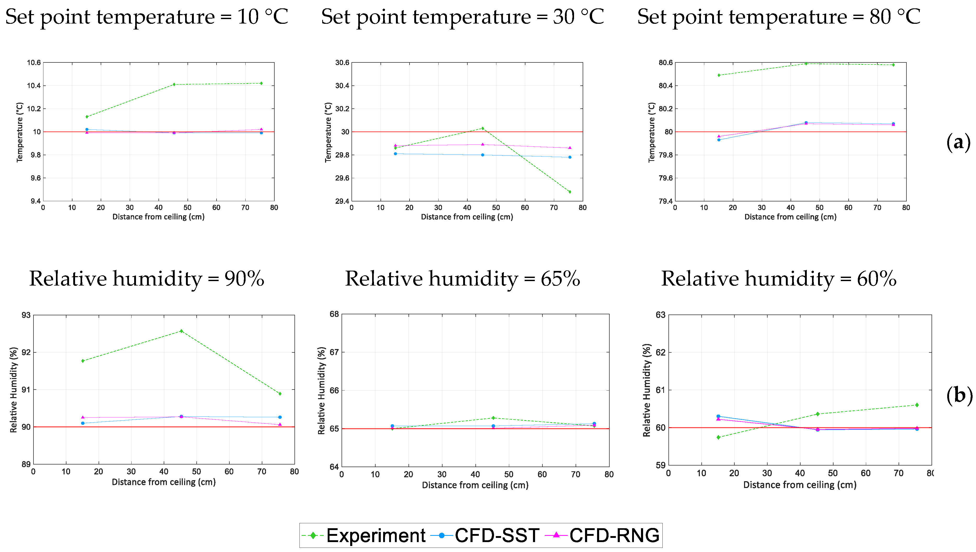
Figure 10 illustrates the comparison of experimental and numerical values for the k−ω SST model and k−ε RNG model for different measured points inside the chamber for different temperature and relative humidity set points: T = 10 °C, RH = 90%; T = 30 °C, RH = 65%; and T = 80 °C, RH = 60%. The results show that there is a small difference between experimental and numerical values, the maximum absolute error being 0.59 and 0.54 °C for temperature and 2.2% and 2.3% for relative humidity, for the k−ω SST and k−ε RNG models, respectively.
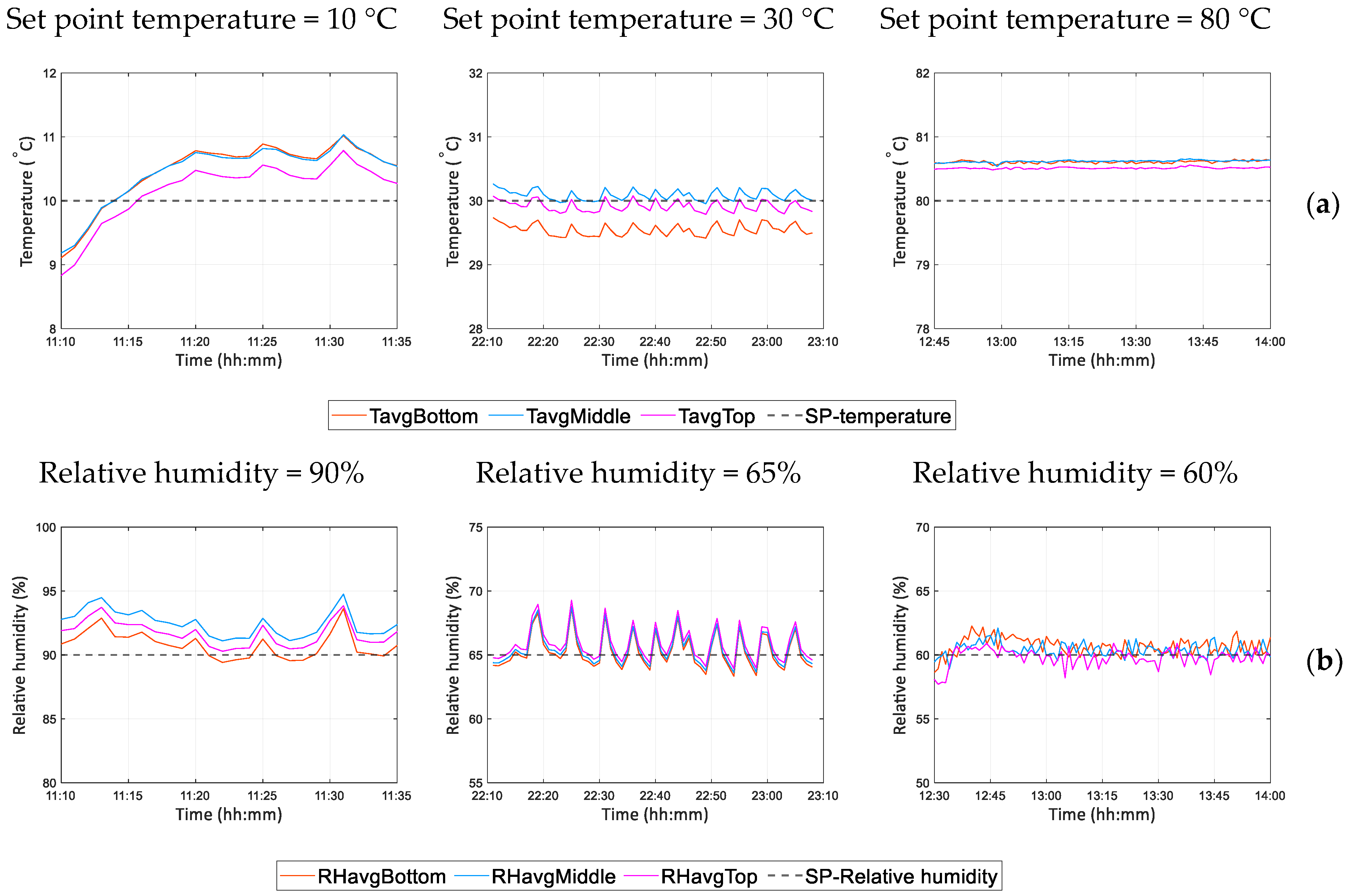
Figure 11 illustrates the measured average temperature and relative humidity for the bottom, middle, and top sections inside the chamber for different temperature and relative humidity set points: T = 10 °C, RH = 90%; T = 30 °C, RH = 65%; and T = 80 °C, RH = 60%. The negligible differences between the recorded values from different sections of the inner chamber show the homogeneous distribution of temperature and relative humidity inside the chamber.
5. Results and Analysis
The thermofluidic performance of the climatic chamber was analysed by means of several simulations for the varying temperature of the air flow inside the inner chamber. The results for the velocity and temperature field are presented in the next sections, and the thermal loss variation with the air temperature is obtained.
5.1. Velocity Field
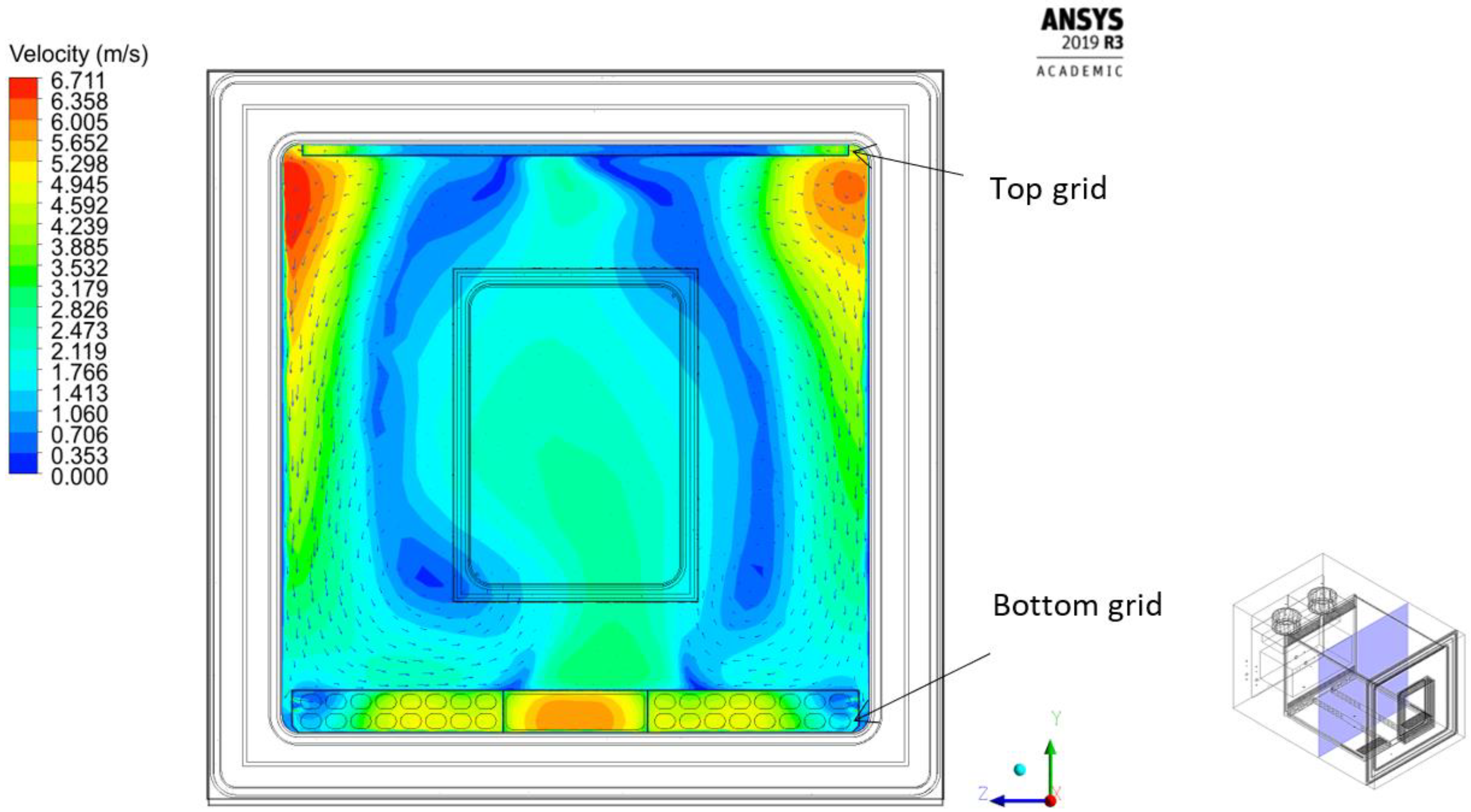
Figure 12 shows the results from the simulated velocity field over the vertical midplane of the chamber for the k−ω SST model. The velocity field shows the presence of the high-velocity zones around the top corners of the chamber. This is related to the fans’ rotating direction, which causes high momentum of the air flow as it enters the inner chamber, mostly from the top corners.
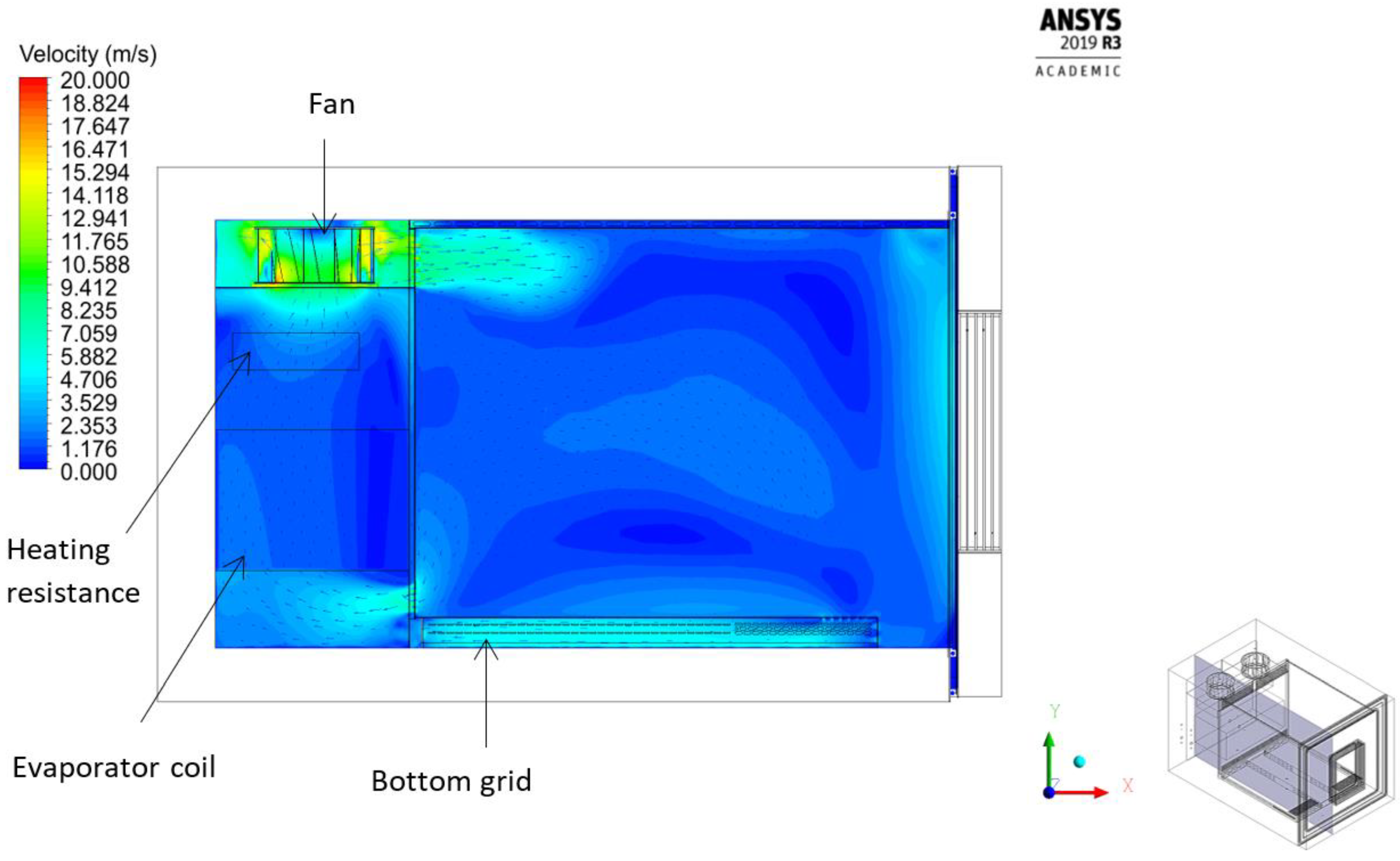
Figure 14 shows the velocity field over the lateral plane, cutting half the left fan, using the k−ω SST model. As predicted, the high velocity zones occur around the inflow and outflow of the test zone. However, a homogeneous air flow persists over the central zone of the test box. Therefore, it can be expected that it would be the best location to keep the specimens during testing, given the uniform velocity field and hence uniform temperature distribution.
5.2. Humidity Field
Figure 15 illustrates the relative humidity distribution inside the chamber on the lateral midplane for temperature and relative humidity set points of 80 °C and 60%, respectively, for the k−ω SST model. It shows that the relative humidity is able to be diffused homogeneously throughout the chamber and stay in the desired set point. The highest concentration of humidity is observed in the top region of the chamber, above the top grid, and around the bottom area of the door, where the velocity field is around zero.
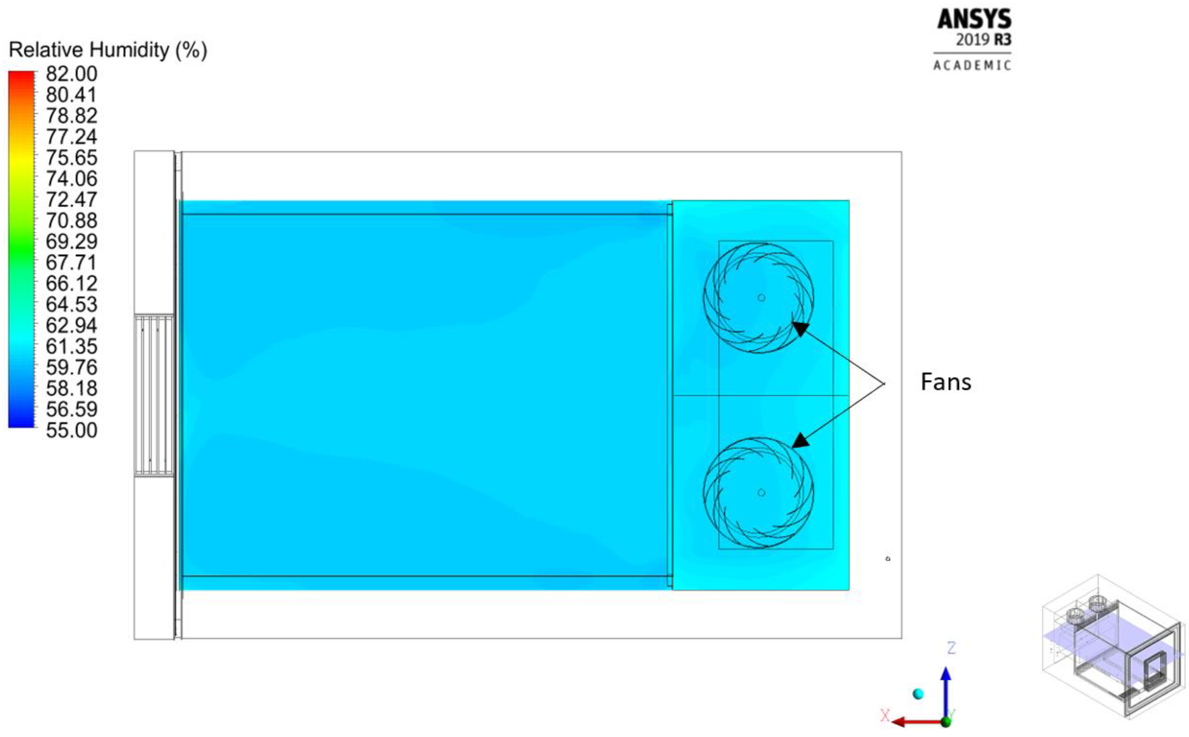
The humidity field inside the chamber is shown from the top view on the horizontal midplane for the k−ω SST model in
Figure 16. It shows an excellent humidity distribution in the middle region of the chamber with a standard deviation of 0.15% of relative humidity.
5.3. Temperature field
The temperature field was simulated for several fixed air temperatures inside the chamber (considering the humidity system is off).
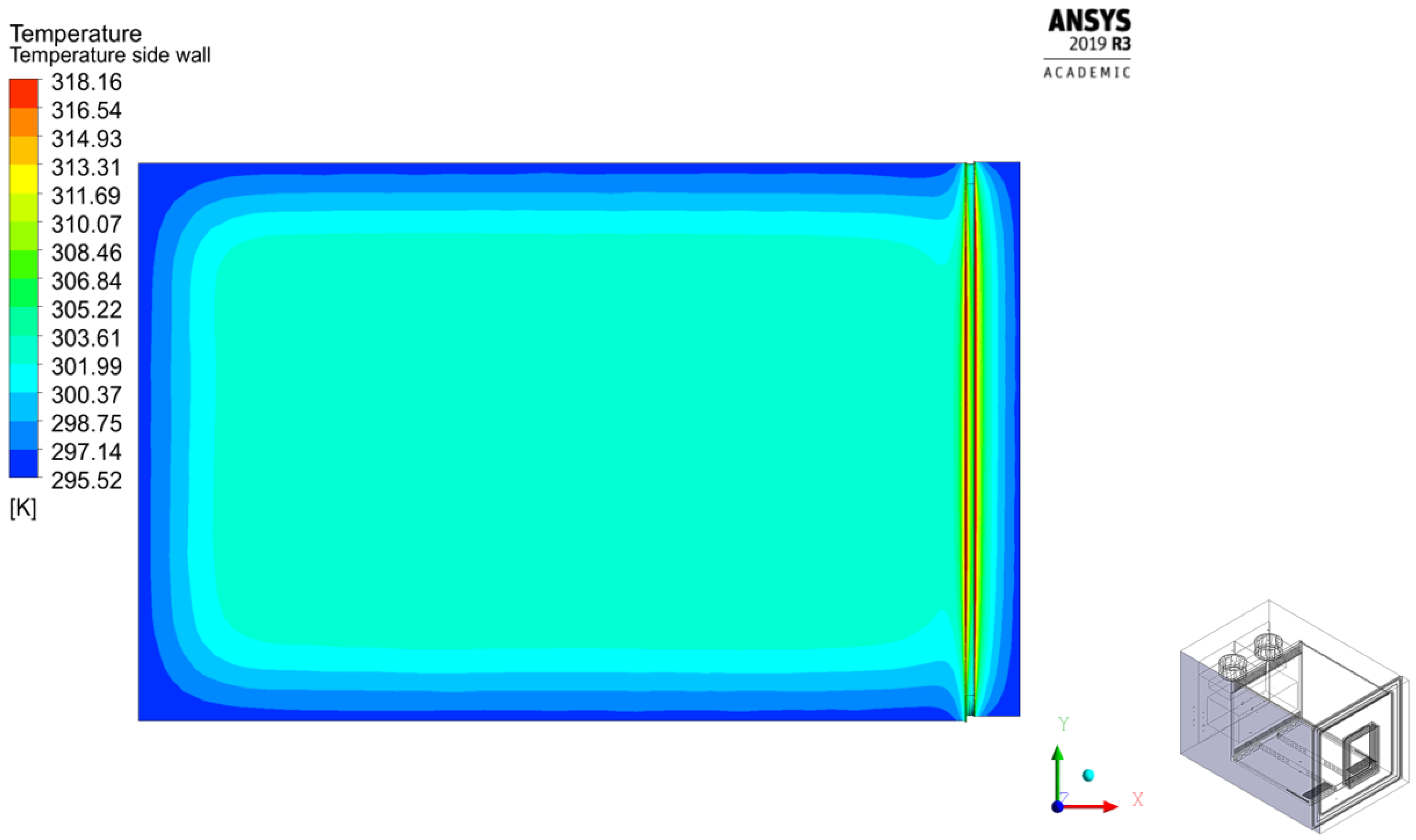
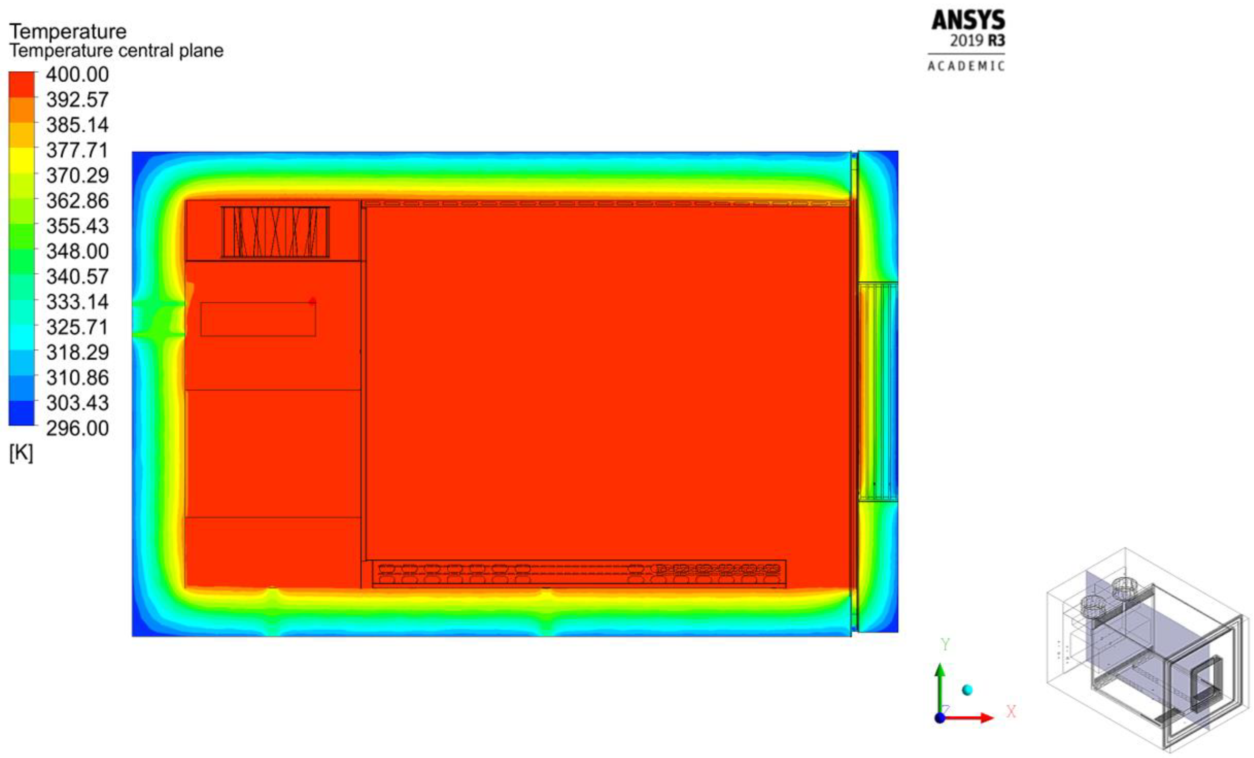
Figure 17 shows the temperature field for an inside temperature equal to 120 °C on the outside surface of the side wall of the chamber for the k−ω SST model, which represents the predicted thermal bridge at the door–wall junction.
The temperature distribution for an inside temperature equal to 120 °C on the vertical midplane of the chamber for the k−ω SST model is shown in
Figure 18. From this result, it can be predicted that the temperature field is able to remain homogeneous inside the chamber during steady-state operation. It also shows how using the six-layer window is effective in reducing heat loss from the chamber.
The computations were repeated for all mentioned turbulence models. As shown in
Table 3, negligible differences were found in the final outputs using the different turbulence models.
5.4. Thermal Losses
The thermal losses from the chamber to the outside air were obtained for several fixed inner temperatures and for an external temperature of 22 °C. The results for the various components surrounding the inner chamber for a fixed inside temperature of 120 °C are shown in
Table 4. The results show that 92% of the thermal loss of the chamber is through the insulation surrounding the external walls and door, which is mainly due to the large side area of the chamber (1258 m
2) compared with the other components (33.3 m
2). Heat loss through the thermal bridge created by the metal panel in the wall–door junction is responsible for 3.6% of the total heat loss. The smallest heat losses were recorded for the glass window and piping (including the fans’ motors connecting shafts) with 2.7% and 1% of the total heat loss, respectively.
The total heat loss was also determined experimentally by recording the inside and outside temperature of the chamber as well as the energy consumption for a period of 2 days, and used the following equation (according to standard EN12897):
where
is permanent energy losses in (kWh/24 h),
E is electrical energy consumption over a period of 24 h in (kWh/24 h),
is the interior temperature of the chamber over a period of 24 h in “°C”, and
is the ambient temperature of the chamber for a 24 h period in “°C”. The total heat losses for days 1 and 2 were calculated to be 665.15 and 791.32 W, respectively. Therefore, the average heat loss was 728.24 W, which is in good agreement with the numerical result (6% error).
To examine the effect of thermal insulation on the thermal performance of the chamber, the current thermal insulation was replaced by polyurethane insulation, and the total heat loss was calculated. The thermal and physical properties of polyurethane are listed in
Table 2.
The simulations were repeated for different set point temperatures for both rock−wool and polyurethane. The total heat loss from the walls considering polyurethane as the thermal insulation was determined to be 728.44 W for a temperature set point of 120 °C, which shows a 6.4% decrease in the thermal loss from the walls compared with the rock−wool.
Figure 19 shows that the total heat loss from the chamber increases as a linear function with the air temperature inside the chamber. Therefore, as expected, the higher the set point temperature, the higher the predicted thermal loss.
5.5. Changing the Air Flow Pattern
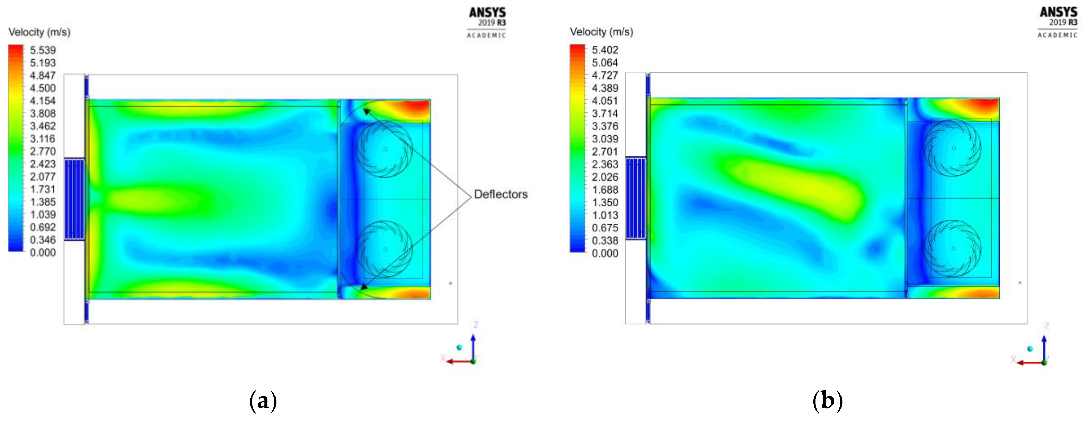
Two different configurations were modelled numerically to optimise the air flow pattern inside the chamber: changing the fans’ rotation direction and adding two deflectors behind the fans.
Figure 20 shows the velocity field on the lateral and horizontal midplane of the chamber for both configurations. It shows that the inclusion of deflectors has a very small effect on the air flow field in the chamber. It also demonstrates that by reversing the fans’ rotation direction, the velocity field shows an asymmetric pattern over the chamber, which can be explained by the asymmetric position of the evaporator. The standard deviations of velocity over the central midplane of the chamber were found to be equal to 1.19 and 1.75 m/s in the presence of deflectors and in inverting the fans’ rotation, respectively.
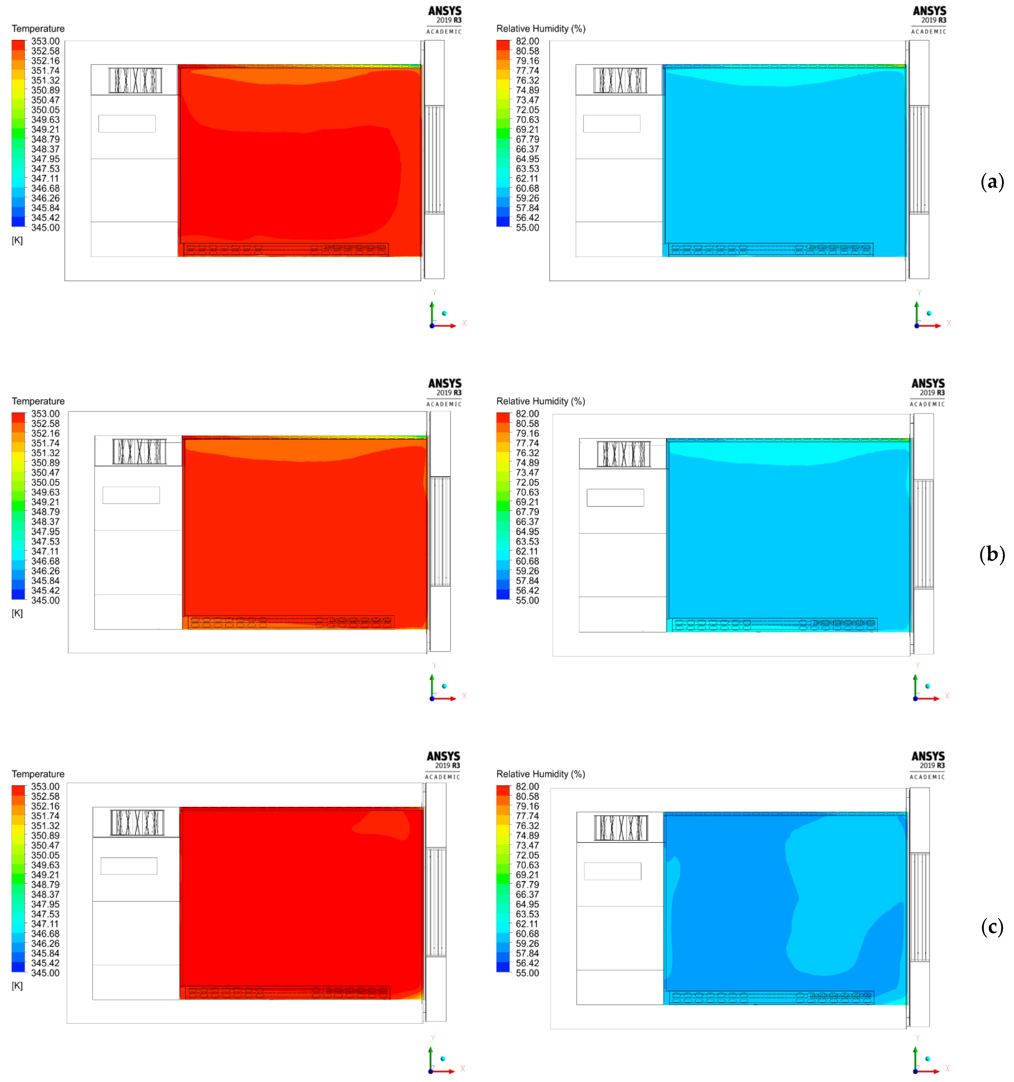
The temperature and relative humidity fields on the lateral midplane of the chamber are presented in
Figure 21 for both configurations, for temperature and humidity set points of 80 °C and 60%, respectively. Despite the asymmetric air flow circulation in the chamber, the better temperature distribution resulted from the fans with inverse rotation with a standard deviation of 0.43 °C. This behaviour is probably due to a higher air flow velocity, which helps create a uniform air distribution inside the testing area. With the deflectors added, the temperature and relative humidity distribution are almost identical to the current design, so attaching the deflectors is unnecessary. Even though reversing the rotation of the fans will produce a better temperature distribution, the current design offers a more uniform air flow within the chamber than either of the two other configurations.
6. Conclusions
In this study, a thermofluidic 3D model of a climate chamber was developed using Ansys Fluent and validated with experimental data. The numerical modelling was carried out using four different turbulence models: k−ω SST, k−ε RNG, k−ε realisable, and k−ε standard. The numerical results showed good agreement with the experimental data, with an average absolute error of 0.67 m/s resulting from the k−ε RNG model for the velocity. The CFD model demonstrated a homogeneous air flow inside the test zone of the chamber for all the turbulence models. Additionally, a uniform temperature distribution over the test zone with a standard deviation of 0.61 °C (for the k−ω SST model) was predicted. The relative humidity distribution inside the chamber was also modelled using a transport species approach. A homogeneous distribution of humidity was found inside the chamber with a standard deviation of 0.72% (for the k−ω SST model) inside the testing area. Furthermore, the thermal losses through the external components of the chamber, including the walls, front window, wall–door junction, and piping, were modelled, showing that the maximum heat loss was via the walls (720.08 W), followed by the thermal bridge created by the wall–door junction (28.24 W), which was in good agreement with the experimental data, with approximately 6% error. The model was simulated using polyurethane thermal insulation instead of the current rock−wool insulation as a further measure for improvement. The results showed a slight decrease (6.4%) in the total thermal loss from the chamber’s walls. Finally, two strategies for modifying the air flow were proposed, by considering deflectors and inverting the fans’ rotation. It was concluded that reversing the fans’ rotation will result in a better general temperature distribution. Still, the current design appears to outperform both the proposed chamber configurations when it comes to a more uniform air flow within the chamber.
Author Contributions
Conceptualization, B.R., A.T., T.J., M.B. and J.M.; methodology, B.R., A.T., T.J., M.B.; software, B.R.; validation, T.J. and M.B.; formal analysis, B.R., A.T., T.J., M.B. and J.M.; investigation, B.R., M.B.; resources, B.R., A.T., T.J., M.B. and J.M.; data curation, B.R., A.T., T.J. and M.B.; writing—original draft preparation, B.R., M.B. and T.J.; writing—review and editing, B.R., A.T. and M.B.; visualization, T.J., M.B. and J.M.; supervision, A.T.; project administration, A.T.; funding acquisition, A.T. All authors have read and agreed to the published version of the manuscript.
Funding
This research is part of the Project TESTA+ More volume, the same technology (POCI-01-0247-FEDER-038356/LISBOA-01-0247-FEDER-038356) funded by the Operational Program for Competitiveness and Internationalization (POCI) of Portugal 2020, with the support of the European Regional Development Fund (FEDER).
Data Availability Statement
The data presented in this study are available on request from the corresponding author. The data are not publicly available due to companies’ privacy policy.
Conflicts of Interest
The authors declare no conflict of interest.
References
- Liang, Y.Y.; Hu, J.C.; Chen, J.P.; Shen, Y.G.; Du, J. A transient thermal model for full-size vehicle climate chamber. Energy Build. 2014, 85, 256–264. [Google Scholar] [CrossRef]
- Dostál, J.; Ferkl, L. Model Predictive Control of Climatic Chamber with On-off Actuators. IFAC Proc. Vol. 2014, 47, 4423–4428. [Google Scholar] [CrossRef] [Green Version]
- García-Contreras, R.; Gómez, A.; Fernández-Yáñez, P.; Armas, O. Estimation of thermal loads in a climatic chamber for vehicle testing. Transp. Res. Part D Transp. Environ. 2018, 65, 761–771. [Google Scholar] [CrossRef]
- Mensah, K.; Byeong, M.Y.; Min, C.J.; Yoon, S. Study on the performance of a temperature and humidity chamber. In Proceedings of the Korean Society of Mechanical Engineers (KSME) Conference, Yeosu, South Korea, April 2016; pp. 351–352. [Google Scholar]
- Candanedo, L.; Handfield, L.; Karava, P.; Bessoudo, M.; Tzempelikos, A.; Athienitis, A. Airflow and thermal simulation in a controlled test chamber with different heating configurations using CFD modeling. In Proceedings of the 2nd Canadian Solar Buildings Conference, Calgary, AB, Canada, 10–14 June 2007. [Google Scholar]
- Lecoq, L.; Flick, D.; Plana-Fattori, A.; Laguerre, O. Characterization of evaporation rate, temperature, velocity and humidity fields in a cold chamber. In Proceedings of the 3rd IIR International Conference on Sustainability and the Cold Chain, London, UK, 23–25 June 2014; pp. 267–274. [Google Scholar]
- Rogié, B.; Jensen, J.K.; Hansen, S.O.K.; Markussen, W.B. Analysis of Cold Air Recirculation in the Evaporators of Large-Scale Air-Source Heat Pumps Using CFD Simulations. Fluids 2020, 5, 186. [Google Scholar] [CrossRef]
- Liu, Y.; Liu, S.; Zhang, H. Numerical Simulation of Heat and Moisture Transfer in Deep Air Buried. Procedia Eng. 2017, 205, 1927–1933. [Google Scholar] [CrossRef]
- Vojkuvkova, P.; Sikula, O.; Weyr, J. Assessment of condensation of water vapor in the mixing chamber by CFD method. EPJ Web Conf. 2015, 92, 02112. [Google Scholar] [CrossRef] [Green Version]
- Shojaee Nasirabadi, P.; Jabbari, M.; Hattel, J.H. CFD simulation and statistical analysis of moisture transfer into an electronic enclosure. Appl. Math. Model. 2017, 44, 246–260. [Google Scholar] [CrossRef]
- Silva, R.; Brett, M.; Ferreira, A.D.; Serra, C.; Jesus, T.; Fino, M.; Tadeu, A.; Mendes, J.; Araújo, J.; Santos, R. Computational Fluid Dynamics Modelling and Experimental Validation of the Thermofluidic Performance of Climatic Chambers. J. Therm. Sci. Eng. Appl. 2020, 12, 021014. [Google Scholar] [CrossRef]
- Ferziger, J.H.; Peric, M. Computational Methods for Fluid Dynamics, 3rd ed.; Springer: Berlin/Heidelberg, Germany, 2012. [Google Scholar]
- Versteeg, H.K.; Malalasekera, W. An Introduction to Computational Fluid Dynamics: The Finite Volume Method, 2nd ed.; Pearson Education: Glasgow, UK, 2007. [Google Scholar]
- Tu, J.; Yeoh, G.H.; Liu, C. Computational Fluid Dynamics: A Practical Approach, 2nd ed.; Butterworth Heinemann: Oxford, UK, 2012. [Google Scholar]
- Karypis, G.; Kumar, V. A Software Package for Partitioning Unstructured Graphs, Partitioning Meshes, and Computing Fill-Reducing Orderings of Sparse Matrices; University of Minnesota, Department of Computer Science and Engineering, Army HPC Research Center: Minneapolis, MN, USA, 1998. [Google Scholar]
- Karypis, G. METIS and ParMETIS. In Encyclopedia of Parallel Computing; Padua, D., Ed.; Springer: Boston, MA, USA, 2011; pp. 1117–1124. [Google Scholar] [CrossRef]
- ANSYS, Inc. ANSYS FLUENT 12.0/12.1 Documentation. Available online: https://www.afs.enea.it/project/neptunius/docs/fluent/ (accessed on 26 August 2021).
- Cengel, Y.A.; Cimbala, J.M. Fluid Mechanics-Fundamentals and Applications; McGraw-Hill Higher Education: Boston, MA, USA, 2006. [Google Scholar]
- Menter, F.R.; Kuntz, M.; Langtry, R.B. Ten years of industrial experience with the SST turbulence model. Heat Mass Transf. 2003, 4, 625–632. [Google Scholar]
- Durbin, P.A.; Reif, B.A. Reynolds Averaged Navier-Stokes Equations. Statistical Theory and Modeling for Turbulent Flow, 2nd ed.; John Wiley & Sons, Ltd.: London, UK, 2010; pp. 45–56. [Google Scholar] [CrossRef]
- Bergman, T.L.; Lavine, A.S.; Incropera, F.P.; Dewitt, D.P. Fundamentals of Heat and Mass Transfer, 7th ed.; John Wiley & Sons: Hoboken, NJ, USA, 2011. [Google Scholar]
- Churchill, S.W.; Chu, H.H.S. Correlating equations for laminar and turbulent free convection from a vertical pate. Int. J. Heat Mass Transf. 1975, 18, 1323–1329. [Google Scholar] [CrossRef]
- Rich, B.R. An investigation of heat transfer from an inclined flat plate in free convection. Trans. ASME 1953, 75, 489–499. [Google Scholar]
- Shah, R.K.; Sekulic, D.P. Fundamentals of Heat Exchanger Design; John Wiley & Sons: Hoboken, NJ, USA, 2003. [Google Scholar] [CrossRef]
- Keenan, J.H.; Chao, J.; Kaye, J. Gas Tables: International Version, 2nd ed.; John Wiley & Sons: Hoboken, NJ, USA, 1983. [Google Scholar]
- Touloukian, Y.S. Thermophysical Properties of Matter: The TPRC Data Series; A Comprehensive Compilation of Data; Purdue University, Thermophysical and Electronic Properties Information Center: Lafayette, IN, USA, 1970; Volume 1. [Google Scholar]
- Engineering Toolbox. Available online: http://www.engineeringtoolbox.com (accessed on 16 March 2021).
- Abdou, A.A.; Budaiwi, I.M. Comparison of thermal conductivity measurements of building insulation materials under various operation temperatures. J. Build. Phys. 2005, 29, 171–184. [Google Scholar] [CrossRef]
Figure 1.
Climatic chamber prototype under development: external and internal view.
Figure 1.
Climatic chamber prototype under development: external and internal view.
Figure 2.
The geometry of the climatic chamber.
Figure 2.
The geometry of the climatic chamber.
Figure 3.
Polyhedral mesh—3D view: (a) and cross-sectional view (b).
Figure 3.
Polyhedral mesh—3D view: (a) and cross-sectional view (b).
Figure 4.
Mesh refinement in bottom: (a) and back (b) perforated grids.
Figure 4.
Mesh refinement in bottom: (a) and back (b) perforated grids.
Figure 5.
Radial fan characteristic curve.
Figure 5.
Radial fan characteristic curve.
Figure 6.
Convergence of scaled residuals: (a) k−ω SST model; (b) k−ε RNG model.
Figure 6.
Convergence of scaled residuals: (a) k−ω SST model; (b) k−ε RNG model.
Figure 7.
Convergence of monitored variables: (a) k−ω SST; (b) k−ε RNG model.
Figure 7.
Convergence of monitored variables: (a) k−ω SST; (b) k−ε RNG model.
Figure 8.
Positions of the monitoring points.
Figure 8.
Positions of the monitoring points.
Figure 9.
Comparison between numerical modelling and experimental outputs: (a) left column, (b) centre column, (c) right column.
Figure 9.
Comparison between numerical modelling and experimental outputs: (a) left column, (b) centre column, (c) right column.
Figure 10.
Comparison between numerical modelling and experimental outputs: (a) temperature; (b) relative humidity inside the chamber for different set points, experimental vs. numerical results.
Figure 10.
Comparison between numerical modelling and experimental outputs: (a) temperature; (b) relative humidity inside the chamber for different set points, experimental vs. numerical results.
Figure 11.
Measured (a) temperatures; (b) relative humidity inside the climatic chamber (SP-temperature: set point temperature; SP-relative humidity: set point relative humidity; TavgBottom: average temperature, bottom section of inside chamber; RHavgBottom: average relative humidity, bottom section of inside chamber; TavgMiddle: average temperature, middle section of inside chamber; RHavgMiddle: average relative humidity, middle section of inside chamber; TavgTop: average temperature, top section of inside chamber; RHavgBottom: average relative humidity, top section of inside chamber).
Figure 12.
Front view of the velocity field in the vertical midplane (x/W = 0.4) obtained using the k−ω SST model The asymmetry in the fluid flow can be explained by the evaporator not being positioned symmetrically, and so it allows more fluid flow from one side than from the other.
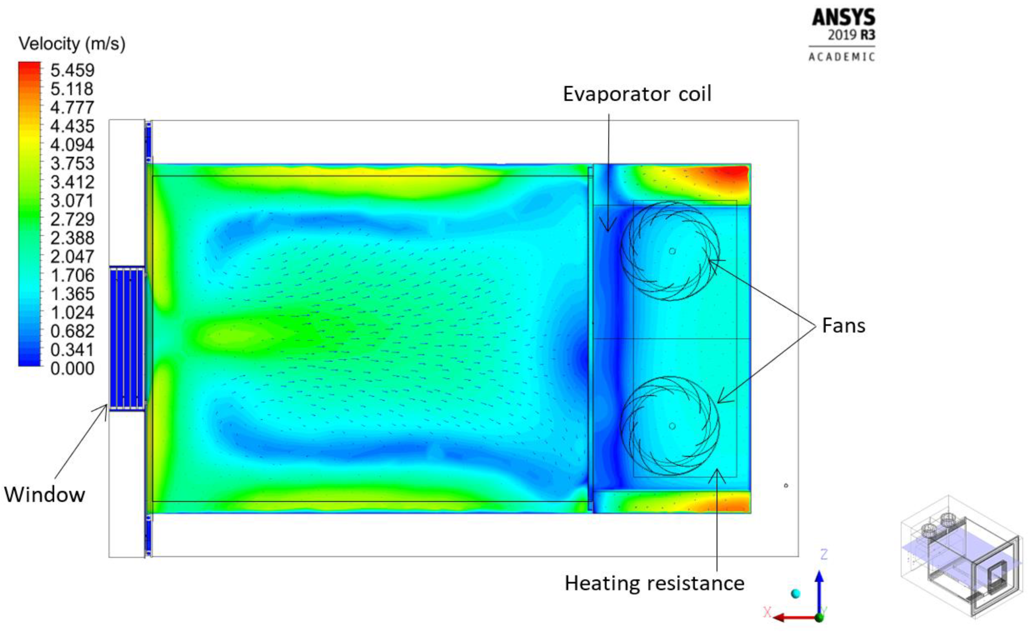
Figure 13 shows the details of the asymmetric position of the evaporator in the chamber and the velocity field viewed from above for the k−ω SST model.
Figure 13.
Top view of the velocity field on the horizontal midplane (y/H = 0.12) obtained using the k−ω SST model.
Figure 13.
Top view of the velocity field on the horizontal midplane (y/H = 0.12) obtained using the k−ω SST model.
Figure 14.
Lateral view of the velocity field in the vertical plane cutting half the left fan (z/L = 0.25) obtained using the k−ω SST model.
Figure 14.
Lateral view of the velocity field in the vertical plane cutting half the left fan (z/L = 0.25) obtained using the k−ω SST model.
Figure 15.
Relative humidity distribution on the lateral midplane (z/L = 0.5) obtained using the k−ω SST model.
Figure 15.
Relative humidity distribution on the lateral midplane (z/L = 0.5) obtained using the k−ω SST model.
Figure 16.
Top view of the relative humidity distribution on the horizontal midplane (y/H = 0.12) obtained using the k−ω SST model.
Figure 16.
Top view of the relative humidity distribution on the horizontal midplane (y/H = 0.12) obtained using the k−ω SST model.
Figure 17.
Temperature field on the side wall of the chamber obtained using the k−ω SST model.
Figure 17.
Temperature field on the side wall of the chamber obtained using the k−ω SST model.
Figure 18.
Temperature distribution on the lateral midplane (z/L = 0.5) obtained using the k−ω SST model.
Figure 18.
Temperature distribution on the lateral midplane (z/L = 0.5) obtained using the k−ω SST model.
Figure 19.
Variation of total heat loss of the chamber with the inside temperature (rock−wool vs. polyurethane).
Figure 19.
Variation of total heat loss of the chamber with the inside temperature (rock−wool vs. polyurethane).
Figure 20.
Top view of the velocity field on the horizontal midplane (y/H = 0.12): (a) fans with added deflectors; (b) fans with inverse rotation.
Figure 20.
Top view of the velocity field on the horizontal midplane (y/H = 0.12): (a) fans with added deflectors; (b) fans with inverse rotation.
Figure 21.
Temperature and relative humidity distribution in the testing area on the lateral midplane (z/L = 0.5): (a) current design, (b) fans with deflectors, (c) fans with inverse rotation.
Figure 21.
Temperature and relative humidity distribution in the testing area on the lateral midplane (z/L = 0.5): (a) current design, (b) fans with deflectors, (c) fans with inverse rotation.
Table 1.
Specifications of the climatic chamber.
Table 1.
Specifications of the climatic chamber.
| Temperature range | 10–90 °C |
| Temperature precision | In time ≤ ±0.5 °C
In space ≤ ±1.5 °C |
| Humidity range | 10% RH to 98% RH |
| Humidity precision | In time ≤ ±1.0% RH
In space ≤ ±2.5% RH |
| Heating | Tubular stainless steel electric heaters (details in Section 3.2) |
| Cooling | Air-cooled hermetic scroll compressor group with enforced ventilation |
| Humidity control system | Humidity: thermostatic bath with dew point control
Drying: thermostatic bath with dew point control and additional dry coil |
| Humidity sensors | Psychrometric, capacitive (or both simultaneously) |
| Ventilation | Two fans (details in Section 3.2) |
Table 2.
Properties of the solid materials.
Table 2.
Properties of the solid materials.
| Material | Density (kg/m3) | Thermal Conductivity
(W/(m·K)) | Emissivity (–) |
|---|
| Stainless steel | 8055 (c) | 15.1 (c) | 0.95 (exterior wall) (a); 0.1 (inner wall) (a) |
| Rock−wool | 120 (b) | (e) | (–) |
| Polyurethane | 44 (b) | (e) | (–) |
| Rubber | 1100 (d) | 0.2 (d) | (–) |
| Glass | 2500 (c) | 1 (c) | 0.837 (c) |
| Copper | 8978 (b) | 387.6 (b) | (–) |
Table 3.
Comparison of the average velocities and standard deviation of velocity, temperature, and relative humidity results inside the testing area obtained using the four different turbulence models.
Table 3.
Comparison of the average velocities and standard deviation of velocity, temperature, and relative humidity results inside the testing area obtained using the four different turbulence models.
| Turbulence Model | Average Velocity | Standard Deviation of Velocity | Standard Deviation of Temperature | Standard Deviation of Humidity |
|---|
| k−ω SST | 2.25 m/s | 1.07 m/s | 0.61 °C | 0.72% |
| k−ε RNG | 2.22 m/s | 1.11 m/s | 0.63 °C | 0.76% |
| k−ε realisable | 2.27 m/s | 1.13 m/s | 0.66 °C | 0.74% |
| k−ε standard | 2.14 m/s | 1.14 m/s | 0.67 °C | 0.73% |
Table 4.
Thermal losses.
| Component | Heat Loss (W) |
|---|
| Walls | 720.086 |
| Window | 20.981 |
| Piping | 8.858 |
| Wall–door junction | 28.246 |
| Total | 778.171 |
| Publisher’s Note: MDPI stays neutral with regard to jurisdictional claims in published maps and institutional affiliations. |
© 2021 by the authors. Licensee MDPI, Basel, Switzerland. This article is an open access article distributed under the terms and conditions of the Creative Commons Attribution (CC BY) license (https://creativecommons.org/licenses/by/4.0/).
