Article

On the Characteristics of the Super-Critical Wake behind a Circular Cylinder

1
Turbulence and Aerodynamics Research Group, Universitat Politècnica de Catalunya (UPC), 08221 Barcelona, Spain
2
Barcelona Supercomputing Center, 08034 Barcelona, Spain
*
Author to whom correspondence should be addressed.
Fluids 2021, 6(11), 396; https://doi.org/10.3390/fluids6110396
Submission received: 8 October 2021 / Revised: 22 October 2021 / Accepted: 29 October 2021 / Published: 3 November 2021
(This article belongs to the Special Issue External Aerodynamics)

Abstract

:
The flow topology of the wake behind a circular cylinder at the super-critical Reynolds number of R e = 7.2 × 10 5 is investigated by means of large eddy simulations. In spite of the many research works on circular cylinders, there are no studies concerning the main characteristics and topology of the near wake in the super-critical regime. Thus, the present work attempts to fill the gap in the literature and contribute to the analysis of both the unsteady wake and the turbulent statistics of the flow. It is found that although the wake is symmetric and preserves similar traits to those observed in the sub-critical regime, such as the typical two-lobed configuration in the vortex formation zone, important differences are also observed. Owing to the delayed separation of the flow and the transition to turbulence in the attached boundary layer, Reynolds stresses peak in the detached shear layers close to the separation point. The unsteady mean flow is also investigated, and topological critical points are identified in the vortex formation zone and the near wake. Finally, time-frequency analysis is performed by means of wavelets. The study shows that in addition to the vortex shedding frequency, the inception of instabilities that trigger transition to turbulence occurs intermittently in the attached boundary layer and is registered as a phenomenon of variable intensity in time.

1. Introduction

The flow past a circular cylinder has been the subject of many investigations, as the complexity of the flow—which involves a laminar boundary layer, separation of the flow, the transition to turbulence and the development of a turbulent wake with a periodic vortex shedding—is present in a wide range of engineering applications. Roshko [1], based on velocity measurements, early classified the flow in different regimes as (i) stable periodic laminar vortex shedding regime 40 R e 150 , (ii) transition range 150 R e 300 , and (iii) irregular range 300 R e 10 , 000 + . The Reynolds number is here defined based on the free-stream velocity U r e f , the cylinder diameter D and the fluid kinematic viscosity ν ( R e = U r e f D / ν ). Later, in [2], he reviewed this classification for including larger Reynolds numbers. The range 10 3 R e 10 5 was referred to as the “Schiller–Linke” regime, also known in the literature as the sub-critical regime. For Reynolds numbers R e > 10 5 , the flow was classified as a critical, super-critical, post-critical or transcritical regime [2]. In the critical regime, the flow undergoes a transition with a sudden decrease in the base suction coefficient and the drag. During this transition, an asymmetric wake is formed, followed by a region where the flow recovers its symmetry, giving rise to a narrow wake with a low drag coefficient C D = 0.2 . This regime was called, by Roshko, the super-critical regime. With the further increase in the Reynolds number, the flow enters in the transcritical regime with a turbulent boundary layer, flow separation around 100 ° and a wider wake.
Regarding the super-critical regime, most of the focus of the experimental and numerical studies performed so far has been on measurements of the drag coefficient, pressure coefficient along the cylinder circumference, vortex shedding frequency and observations about the presence of the so-called laminar separation bubble formed in the rear side of the cylinder [2,3,4,5,6,7]. Some interesting characteristics about the behavior of the boundary layer and skin-friction behavior at the cylinder surface from sub-critical to super-critical Reynolds numbers were studied by Cheng et al. [8]. Moreover, aspects regarding the numerical resolution of the near wake and its impact on the solution were also addressed by Ahmadi and Yang [9]. However, contrary to the vast knowledge about the subcritical regime and its wake topology (see, for instance, the experimental works of Cantwell and Coles [10], Unal and Rockwell [11] and Norberg [12] or the numerical studies of Ma et al. [13], Dong et al. [14] and Lehmkuhl et al. [15] to cite some), little is known about the characteristics and the topology of the super-critical wake. Among the few studies that address some of these characteristics can be mentioned the work performed by Rodríguez et al. [16], where some topological aspects related with the mean recirculation region and wake width were analyzed. Later, Yeon et al. [7] performed large eddy simulations (LES) at sub- and super-critical Reynolds numbers. Although for super-critical Reynolds numbers, the mesh used was coarser than that used in Rodríguez et al. [16], the topological characteristics presented, as well as the pressure distribution and aerodynamic coefficients, were in good agreement with those reported in the literature.
Another point of discussion is whether vortex shedding exists in the super-critical regime. Even though different authors measured a coherent vortex shedding frequency in this regime (see, for instance, the experimental works of [3,4,17]), the super-critical wake has traditionally been described as incoherent [2,5,18,19], with turbulent transition at separation. However, as was pointed out in Lehmkuhl et al. [6] and in Rodríguez et al. [16], vortex shedding was detected at super-critical Reynolds numbers in the range of R e = 6.5 × 10 5 8.5 × 10 5 . In these studies, the wake was described as a coherent vortex street more compact than that observed at sub-critical Reynolds numbers. Moreover, the non-dimensional vortex shedding frequency measured in the super-critical regime was around S t = f v s D / U r e f = 0.45 , in agreement with the experimental measurements of Bearman [4] and Schewe [17].
To the knowledge of the authors, there are not studies concerning the near-wake characteristics of super-critical flows, including first and second order statistics. The present work, based on large eddy simulations, attempts to provide a detailed picture of the super-critical wake encountered past a circular cylinder by means of the evaluation of the mean and fluctuating fields. The Reynolds number studied is R e = 7.2 × 10 5 . The characteristics of the unsteady field, including the vortex formation process, are also analyzed via time-frequency analysis and the visualization of the vortical structures in the near wake. The coherent vortex motion is resolved by using the phase-averaging technique, and it is compared to those reported in the sub-critical regime.

2. Materials and Methods

In the present work, large eddy simulations of the flow are carried out. The spatially filtered incompressible governing equations are written as follows:
u ¯ i x i = 0
u ¯ i t + u ¯ i u ¯ j x j ν 2 u ¯ i x j x j + ρ 1 p ¯ x i = T i j x j
In the above equations, · ¯ represents the filtered variables; x i with i = 1 , 2 , 3 (or x ,   y ,   z ) stands for the stream-wise, wall normal and span-wise directions; u ¯ i (or u ,   v ,   w ) are the filtered velocity vector components in these directions; p ¯ is the filtered pressure scalar field; and ρ and ν are the density and kinematic viscosity, respectively.
In Equation (2), T i j = u i u j ¯ u ¯ i u ¯ j is the subgrid scale (SGS) stress tensor. Its deviatoric part is given by the following:
T i j 1 3 T k k δ i j 2 ν s g s 𝒮 ¯ i j
where S ¯ i j is the large-scale rate-of-strain tensor, S ¯ i j = 1 2 g i j + g j i being g i j = u ¯ i / x j the velocity gradient tensor of the resolved scales; and δ i j is the Kronecker delta. To close the formulation, the subgrid-scale viscosity ν s g s should be modeled. In this work, the model proposed by Vreman [20] is used. In this model, the subgrid-scale viscosity is evaluated as follows:
ν S G S = c 𝒢 g i j g i j
and
𝒢 = G 11 G 22 G 12 2 + G 11 G 33 G 13 2 + G 22 G 33 G 23 2
where G i j = Δ 2   g k i g k j , and c is the model constant. In the present formulation, c = 0.1 .
To solve the above governing equations, the code Alya is used [21]. In Alya, the governing equations are discretized by means of a low-dissipation finite-element scheme, which preserves linear and angular momentum together with kinetic energy at a discrete level. For more details on the low-dissipative scheme used, the reader is referred to Lehmkuhl et al. [22]. The pressure-velocity coupling is solved, using a non-incremental fractional-step method, whereas equations are explicitly integrated in time using a fourth-order Runge–Kutta method [23] combined with an eigenvalue-based time-step estimator [24]. The methodology used proved to be suitable on the resolution of turbulent flows (see, for instance, the author’s recent works [25,26,27,28]).

Definition of the Problem and Boundary Conditions

The flow past a circular cylinder at the Reynolds number of R e = 7.2 × 10 5 , which corresponds with the super-critical regime [3,6,16], is here considered. The case is solved in a computational domain of similar dimensions to that used in Rodríguez et al. [16], i.e., the computational domain extends x 1 [ 10 D : 20 D ] in the stream-wise direction and x 2 [ 10 D : 10 D ] in the cross-stream direction, with the cylinder located at ( x 1 , x 2 ) = ( 0 , 0 ) . As for the spanwise direction, it was proven in Rodríguez et al. [16] that a domain size of L x 3 = D is enough to contain the largest scales of the flow at these Reynolds numbers. Thus, in the present computations, a span-wise size of L x 3 / D = 1 is used.
To solve the governing equations, the boundary conditions imposed at the inlet consist of a uniform velocity profile ( u 1 / U r e f , u 2 / U r e f , u 3 / U r e f ) ( 1 , 0 , 0 ) . At the outlet, a pressure-based condition, similar to that used in Rodriguez et al. [26], is set, whereas at the top and bottom boundaries of the domain, a slip condition is prescribed, i.e., the derivative of the tangential velocity components are zero u 1 / n = u 3 / n = 0 and the normal velocity is also set to zero u 2 = 0 . At the cylinder surface, a no-slip boundary condition is defined. In the homogeneous direction ( x 3 ), the flow is considered periodic.
To solve the case, an unstructured mesh is constructed following a similar criteria to that used in the author’s previous work [16]. Here, the mesh composed of 728,780 grid points in the x 1 x 2 plane is extruded in the x 3 (homogeneous) direction, using 128 grid points. Thus, the computational mesh has a size of 93.28 million grid points. In order to well solve the flow at the boundary layer and in the vortex formation zone, the grid points are clustered around the cylinder and the near wake up to x 1 / D = 5 . A brief discussion about the near-wall resolution requirements for wall-resolved LES, how they are met with the current grid and the evaluation of the ratio of the mesh size used and the Kolmogorov scales is presented in Appendix A.

3. Results

Some of the characteristics of the mean flow at super-critical Reynolds numbers were previously investigated by the authors in Lehmkuhl et al. [6] and Rodríguez et al. [16]. The main observations of these studies regarding the super-critical wake can be summarized as follows. (i) The separated shear layers are bent toward the wake centerline, where they interact with each other; the vortex shedding frequency rises up to S t 0.44 . (ii) The super-critical wake is symmetric with two symmetric separation bubbles on each side of the cylinder rear. (iii) Drag and lift fluctuations decrease by about an order of magnitude with respect to the values reported for the sub-critical regime and the onset of the critical one. These observations are now addressed in a more wide context in order to study how these changes affect the dynamics, turbulent statistics and the overall topology of the flow.

3.1. Coherent Structures

As was commented in the Introduction, the flow in the super-critical regime is often described as an incoherent flow with no vortex shedding (see for instance [5]). In fact, in the experiments performed by Schewe [29] in the critical regime up to R e = 4 × 10 5 , the flow was described to be sensitive to small perturbations and thus, difficult to reproduce the experimental results. However, in the super-critical regime Schewe [17] observed that the flow was very stable without low-frequency fluctuations. These observations are in agreement with the results obtained from LES computations by Rodríguez et al. [16], where the wake was described to be coherent with a narrow band energy peak in the spectrum of the lift fluctuations centered at the the vortex shedding frequency of S t = f v s   U r e f / D 0.44 .
In Figure 1, the vortical structures identified by means of iso-contours of the second invariant of the velocity tensor Q [30] are plotted. As can be seen in the figure, a quasi perfect von Karman vortex street is obtained, with vortex tubes running almost in-line with the wake centerline, as can also be observed if the pressure map is plotted (see Figure 2). In agreement with previous studies, the wake behind the cylinder is narrower than that observed in the sub-critical regime, with flow separation occurring in the rear zone of the cylinder. Moreover, the distance between the vortex tubes is quite constant, which points to a quasi-regular vortex shedding process. As is discussed in Section 3.3, vortex shedding is rather regular and is observed to occur at a frequency of S t = 0.458 . This value is in fair agreement with those reported in the experiments of Bearman [4] ( S t = 0.459 ), Schewe [17] ( S t = 0.467 ), Achenbach and Heinecke [31] ( S t = 0.505 ) and in the numerical simulations of Rodríguez et al. [16] ( S t = 0.44 ). An interesting feature of the flow can be seen close to the location where the boundary layers detach from the cylinder. Pressure iso-contours seem to present a more chaotic behavior. A close-up of the flow in the rear zone of the cylinder is presented in Figure 3. In the figure, instantaneous pressure iso-contours are superimposed to the instantaneous vorticity map. It can be observed that pressure iso-contours cluster past the cylinder apex and present an irregular shape close to the cylinder surface. This can be interpreted as instabilities in the attached boundary layer that grow and are amplified. These instabilities eventually trigger the transition to turbulence. The frequency at which this phenomenon occur is discussed in Section 3.3.

3.2. Statistical Results and Mean Wake Characteristics

For computing the flow statistics presented in this section, the flow is advanced in time from an initial zero velocity field up until the statistically steady state is reached. Once the initial transient is over (it represents about 50 time-units, t i m e u n i t s = t U r e f / D ), statistics are collected for about 150 time-units, which account for about 68 vortex shedding cycles.
In 
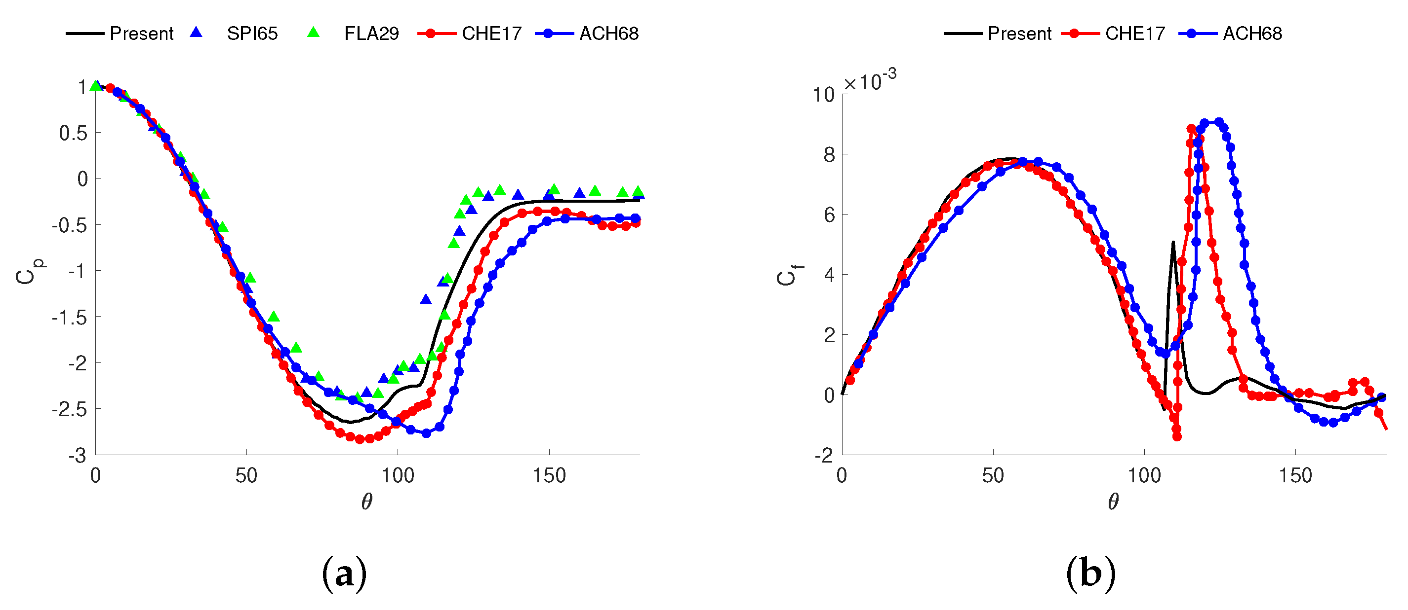
Figure 4, the pressure coefficient ( C p = ( p p r e f ) / 0.5 ρ U r e f 2 with p r e f taken at the inlet) and skin friction coefficient distributions along the cylinder circumference are shown. Present results are plotted against results from the literature. For the pressure coefficient, a plateau is observed around the location where the separation bubble occurs ( ϕ = 99 107 ° ) which is in good agreement with the values reported in the literature as can be seen in the figure and with those reported by Rodríguez et al. [16] ( ϕ = 100 110 ° ). The distribution of the skin friction is also in fair agreement with the literature, although the location of the peak is slightly different. From the skin friction distribution, the separation of the boundary layer can be determined. In our results, this occurs in the rear end of the cylinder at ϕ = 148.8 ° in very good agreement with the values reported in the literature ( ϕ s = 144 ° [3]; ϕ s = 148 ° [16]).
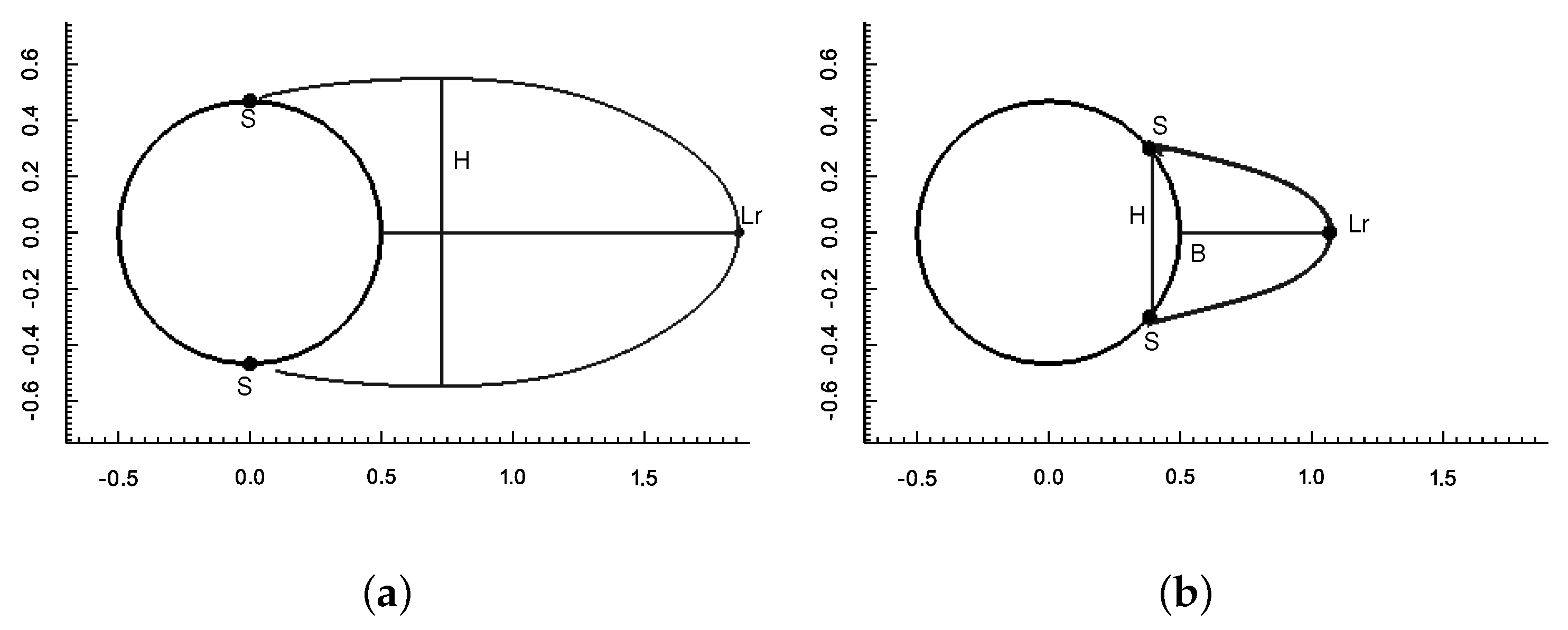
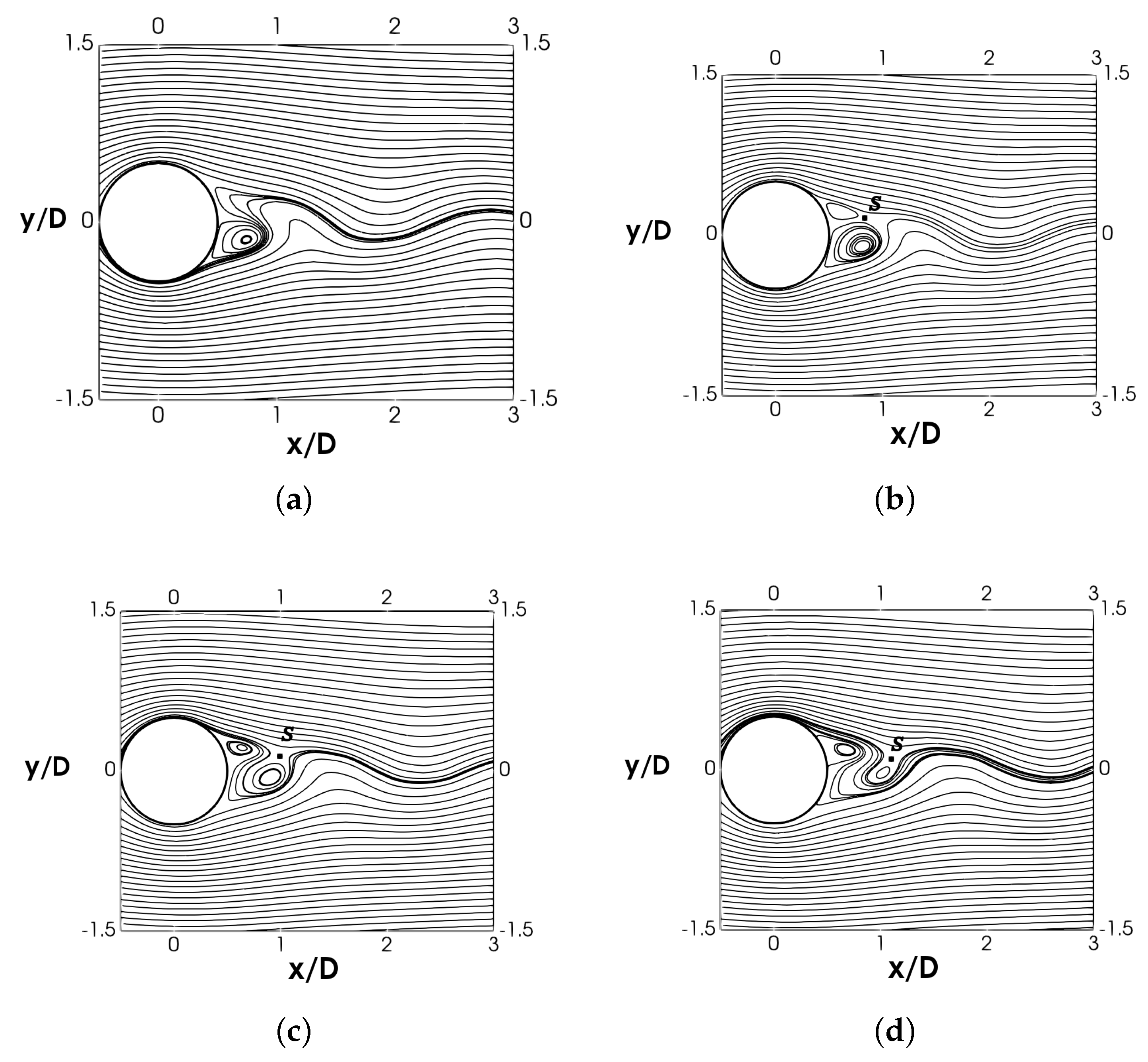
The classical representation of the mean recirculation zone behind a cylinder at the sub-critical Reynolds numbers [2,32] is depicted in Figure 5a. In this representation, this zone is enclosed within the separating flow streamlines. Flow separation (marked as S) occurs near the cylinder apex, whereas the recirculation region is closed somewhere downstream in the wake (marked as L r ). The length of the recirculation zone is then defined as the distance from the cylinder rear to the point in the wake centerline, where the recirculation region is closed ( u 1 = 0 ). The half-height of the recirculation bubble (H) is measured from the wake centerline to the thickest point of the recirculation zone. A similar representation can be made for the super-critical wake (see Figure 5b). In this case, the detachment of the flow (marked as S) is delayed and occurs in the cylinder rear around ϕ 148 . 8 ° (measured from the stagnation point). Owing to the delayed separation, the shear-layers are bent toward the wake centerline. This also is reflected in the separating streamlines, which are closer each other, yielding a smaller recirculation zone. Notice that the half-height of the recirculation zone is measured, in this case, at the separation points (thickest point of the recirculation region) rather than downstream of the cylinder as in the subcritical regime.
In order to analyze the main characteristics of the wake in the super-critical regime, the mean wake is compared to that reported in the sub-critical regime. In particular, it is compared with those obtained by the author’s previous works (Lehmkuhl et al. [15], Aljure et al. [34]), hereafter referred to as LE13 and AL15, respectively, and with the one reported by Cantwell and Coles [10] (hereafter referred to as CC). LE13 and AL15 performed direct numerical simulations of the flow past a cylinder at the subcritical Reynolds numbers of R e = 3900 and R e = 5000 , whereas CC characterized, by means of flying-hot-wire anemometry studies, the near-wake behind a cylinder at the sub-critical Reynolds number of R e = 1.4 × 10 5 . While the former works correspond with Reynolds numbers in the initial part of the sub-critical regime, the latter is at the top part and thus, close to the onset of the critical regime.
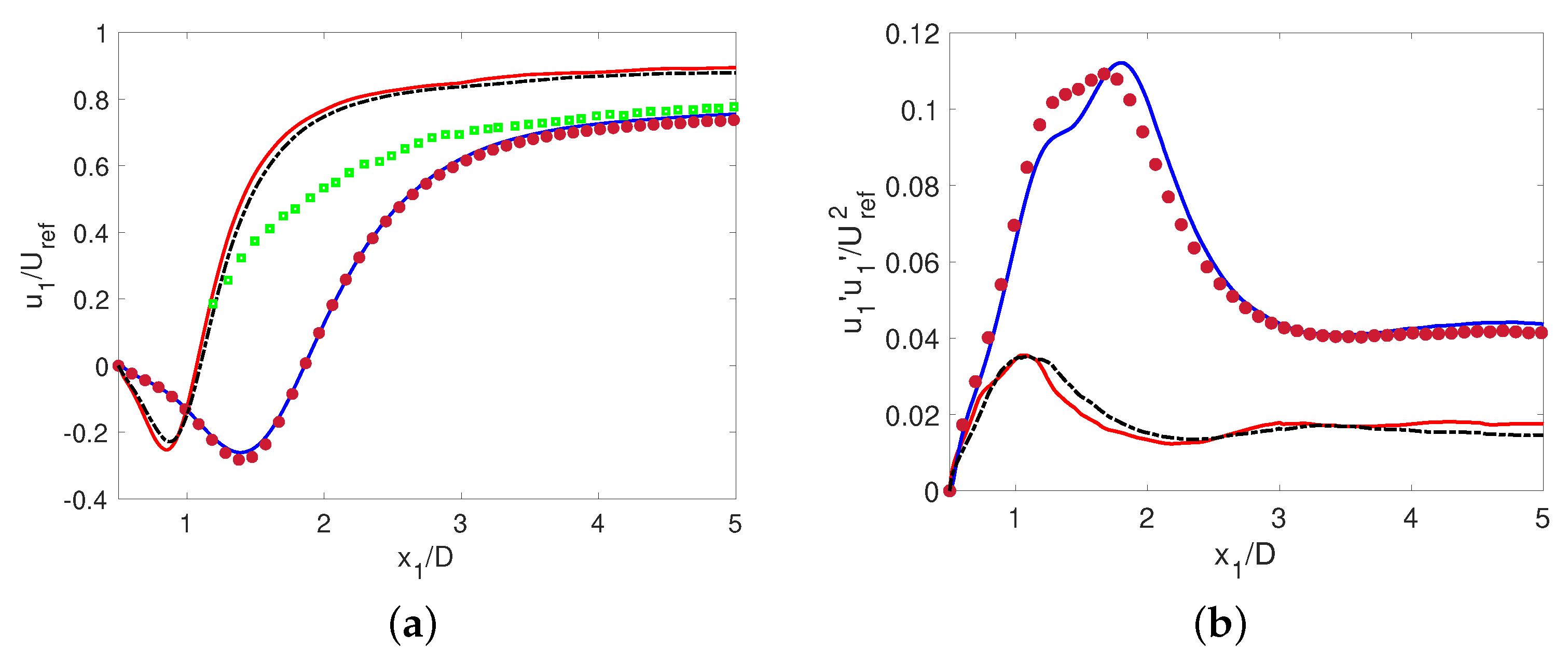
The variation of the stream-wise velocity in the wake centerline together with the normal stream-wise Reynolds stress ( u 1 u 1 ) are plotted in Figure 6. The differences with the sub-critical near wake can be readily observed. The difference in the velocity deficit ( 1 u 1 / U r e f ) after the closure of the recirculation region between these two flow regimes (see Figure 6a) is noticeable. As consequence of the change in the flow separation and thus, in the drag force acting on the cylinder, in the super-critical regime, the velocity deficit (and momentum deficit) caused by the cylinder is lower than that of the sub-critical one. Moreover, when comparing the normal stream-wise Reynolds stresses in the wake centerline, although similar in shape, the peak in the super-critical regime is almost one third that of the sub-critical one, with the peak occurring closer to the cylinder rear end (at x 1 / D = 1.06 ). These differences in the Reynolds stresses can be attributed to the contribution of the coherent component due to the vortex shedding, which is larger in the subcritical regime, rather than to the turbulent fluctuations. In this regime, the shear layers are more separated, and the interaction between each other in the vortex formation zone is more intense. This produces a more energetic vortex shedding, and as a result, larger fluctuations in the flow.
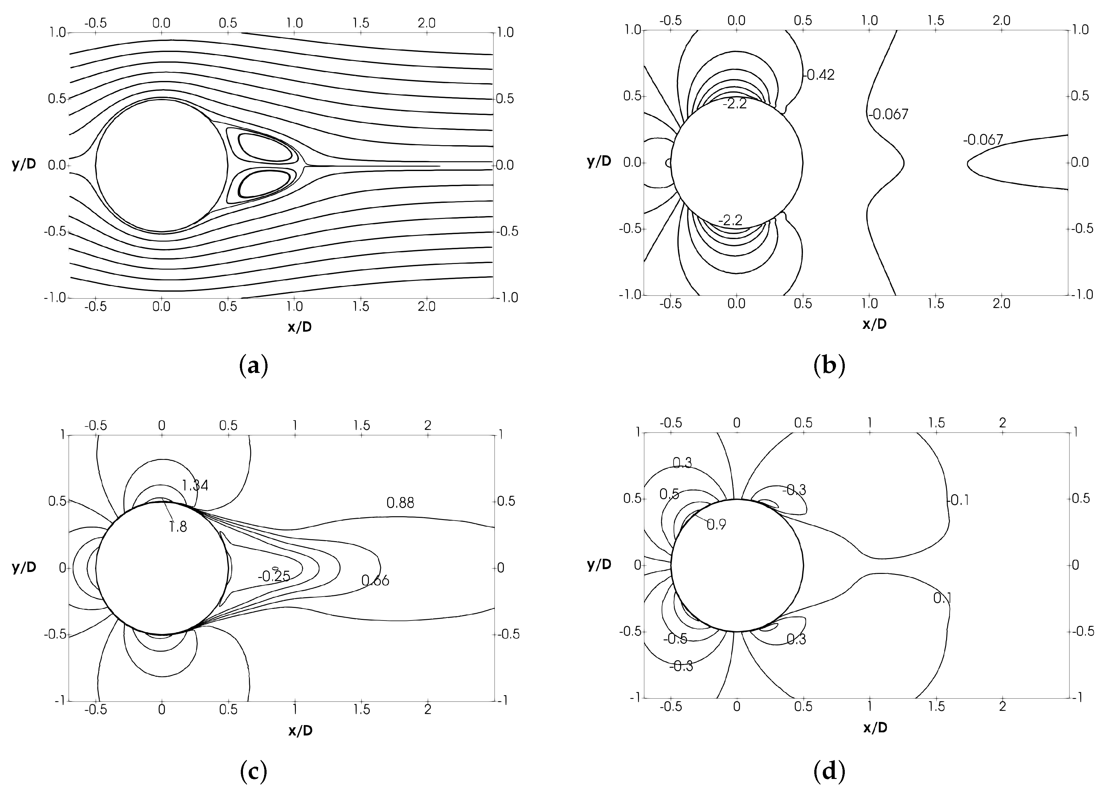
The complete topology of the near wake can be analyzed in Figure 7 and Figure 8. In Figure 7, the mean streamlines, pressure and velocity profiles are shown, whereas in Figure 8, the second-order statistics are given. Complementing these figures, the main statistics extrema in the near wake are given in Table 1, in comparison with similar data for the sub-critical regime. The general topology found is comparable to that of the sub-critical regime as shown by CC and LE13. However, owing to the differences between the sub-critical and super-critical regimes regarding the transition to turbulence, the separation of the shear layers and their interaction, noticeable variations can be observed in the magnitude of the different measured quantities in both the vortex formation region and the wake.
As previously discussed in Rodríguez et al. [16], the recirculation zone is confined to a small region behind the cylinder. This is due to the delayed separation of the boundary layer from the cylinder surface caused by the early transition to turbulence, as it will be further discussed. The length of the recirculation zone is defined as the distance from the cylinder rear end to the point where the stream-wise velocity changes from negative values to positive ones. Here, L r e c / D = 0.57 . In LE13 at R e = 3900 , this zone extends up to x 1 / D = 1.81 ( L r e c / D = 1.31 ), although it is shorter at R e = 1.4 × 10 5 ( L r e c / D = 0.44 according to CC). In fact, the shrinking of the recirculation region with the Reynolds number is a characteristic trait of the sub-critical regime [2]. On the contrary, in the super-critical regime, the length of this zone is almost the same, regardless of the Reynolds number (see, for instance, the values reported in Rodríguez et al. [16]).
Although the near-wake region exhibits the typical two-lobed symmetric pattern (see Figure 7a), it is quite different than that observed at sub-critical Reynolds numbers, where the two main vortices are more separated from each other. On the one hand, the fact that the detached shear layers are bent toward the wake centerline leaves an imprint on both the stream-wise and cross-stream wise velocity fields (see Figure 7c,d). For instance, the streamwise velocity contours are clustered at the shear layers, where there is an important velocity difference between the flow outside and inside the vortex formation zone. However, due to the inclination of the shear layers toward the wake centerline, streamwise velocity contours also follow the same inclination angle of the shear layers. The same applies to the cross-stream wise velocity contours, which follow the closure of the recirculation region. This configuration is different to that observed in the sub-critical regime. As the shear-layers departs from the cylinder are almost parallel to each other (see for instance Figure 6 in [14]), velocity gradients in the shear-layers are only observed in the stream-wise velocity component. On the other hand, the pressure iso-contours are also closer to each other in the vicinity of the separation points, where pressure gradients are the largest. Moreover, the base pressure zone is considerably reduced (in angular size) if it is compared to that observed in the sub-critical regime.
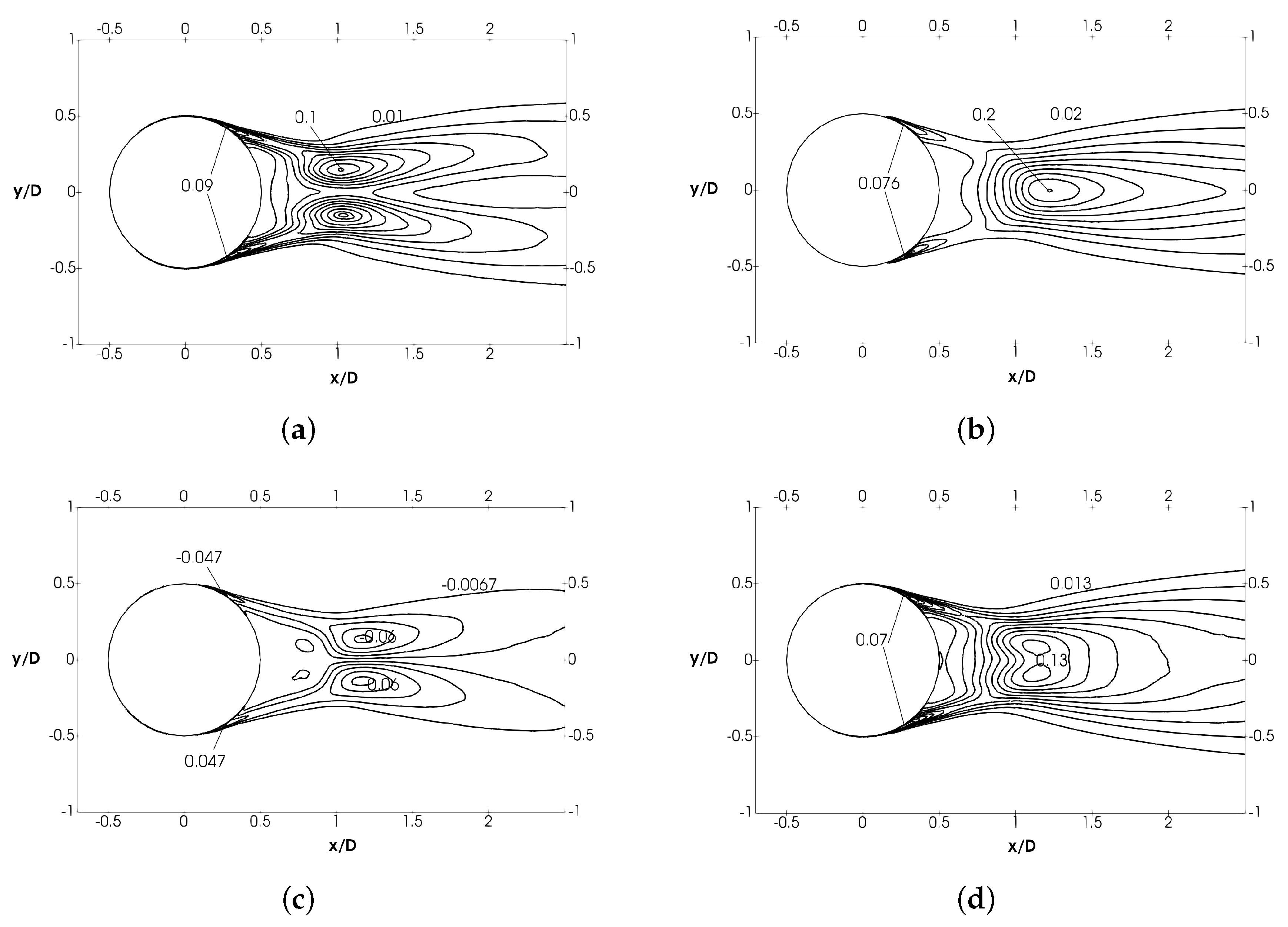
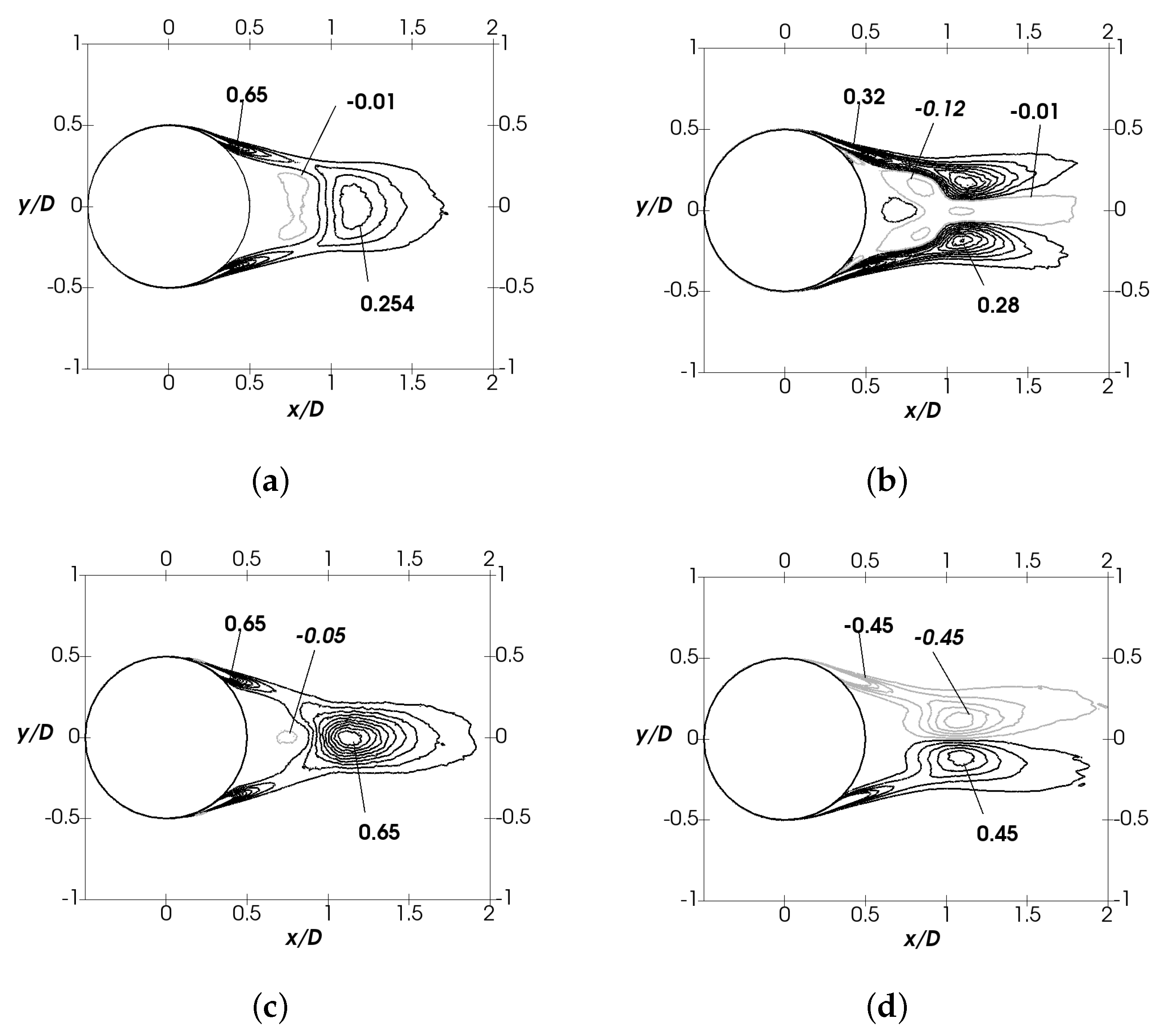
Figure 8 shows the non-dimensional normal and shear stresses together with the turbulent kinetic energy (k) distribution in the near wake. Reynolds stresses are significant along the shear layers and, in particular, reach the highest values before the separation of the boundary layer from the cylinder. In fact, Reynolds stresses become noticeable before the formation of the so-called laminar separation bubble (LSB) that forms in the rear side of the cylinder (see, for instance, Figure 6 in [6]). In the literature, it has always been stated that, in the super-critical regime, the flow separates laminarly from the cylinder surface and, just after separation, the transition to turbulence occurs, which makes the flow reattach to the cylinder, forming a LSB (see, for instance, [16,18,35]). However, as will be further discussed, instabilities in the boundary layer are early triggered, giving rise to rapid transition to turbulence in the attached boundary layer before separation (see the magnitude of the Reynolds stresses and turbulent kinetic energy plotted in Figure 8). This can be appreciated as a characteristic trait of the super-critical regime, i.e., transition to turbulence and the increased momentum transport due to turbulent fluctuations force the boundary layer to keep attached to the cylinder surface much longer, beyond the cylinder apex (the separation location in the sub-critical regime). As a result, it is expected that Reynolds stresses might reach extrema in this region. In fact, both stream-wise normal and shear stresses have a local maximum around the location where the small recirculation bubble closes, i.e., the angular location that corresponds with these peaks is about θ = 113 ° , which is quite close to the location where the laminar recirculation bubble closes ( θ = 111 ° also in agreement with the value reported in Rodríguez et al. [16]). The peak intensities are 0.1 at ( x / D , y / D ) ( 0.19 , 0.469 ) and 0.061 at ( x / D , y / D ) ( 0.211 , 0.461 ) for u 1 u 1 / U r e f 2 and u 1 u 2 / U r e f 2 , respectively.
The other extrema of the Reynolds stresses occur in the near wake region. The magnitude of the normal (stream-wise and cross-stream wise components) are larger than the magnitude of the shear stresses, the cross-stream wise component being the largest of the three, as expected. In Table 1, these magnitudes are compared to those reported in the sub-critical regime. Notice that the non-dimensional fluctuations are, in all cases, lower for the super-critical regime. For instance, the cross-stream wise normal stresses peak is u 2 u 2 / U r e f 2 m a x = 0.43 at R e = 1.4 × 10 5 (as reported by CC), a quantity which is almost the same for the whole sub-critical regime (see Table 1 the values for LE13 and AL15). However, at R e = 7.2 × 10 5 , it is almost half of the value reported for the sub-critical regime, i.e., u 2 u 2 / U r e f 2 m a x = 0.21 . The same can be observed for the other components of the Reynolds stresses. This comes as a consequence of the drag crisis and the change in the behavior of the shear layers. As they are closer to each other, unsteady coherent fluctuations caused by the periodic vortex shedding motion are much lower in magnitude than in the sub-critical regime, where both shear layers are more separated (and parallel to each other). This also can be observed in the fluctuating lift, which drops up to C L = 0.07 in this regime as it was pointed out in Rodríguez et al. [16].
A further insight into the distribution of the turbulent intensities can be obtained if the production of the turbulent kinetic energy and the transport equations is analyzed. For the turbulent kinetic energy, the production term is as follows:
P k = [ u 1 u 1 u 1 x 1 I + u 2 u 2 u 2 x 2 I I + u 1 u 2 ( u 1 x 2 + u 2 x 1 ) I I I ]
For the transport equation for the Reynolds stress tensor, the production term reads as follows:
P i j = u j u k u i x k u i u k u j x k
For the normal and shear stresses u 1 u 1 , u 2 u 2 and u 1 u 2 equations, this turbulent production term can be written as follows:
P 11 = 2 u 1 u 1 u 1 x 1 + u 1 u 2 u 1 x 2
P 22 = 2 u 1 u 2 u 2 x 1 + u 2 u 2 u 2 x 2
P 12 = u 1 u 1 u 2 x 1 u 2 u 2 u 1 x 2
Figure 9 shows contours of the turbulence production for the turbulent kinetic, normal and shear stresses budgets. Production of the turbulent stresses occurs in the shear layers and within the region of 0.5 x 1 / D 2 , which mostly corresponds with the vortex formation zone. The largest values of the turbulent kinetic energy in the shear layers come from the production in the zone; the major contribution stem comes from the production of the cross-stream wise normal stresses. Within the wake, the plots show that the peak in the turbulent kinetic energy (Figure 8d) also coincides with the large values of production (see Figure 9a). The maximum occurs in the wake centerline at x 1 / D = 1.137 , just after the end of the recirculation zone ( x 1 / D = 1.069 ) and very close to the location where turbulent kinetic energy peaks ( x 1 / D = 1.18 ). This is consistent with the observations of CC, where the authors observed that a sharp peak in P k is produced near the closure point of the mean streamline pattern.
In the vortex formation region, the turbulent production of the stream-wise normal stresses is mostly negative near the wake centerline (see Figure 9b). This might be associated with the work of u 1 u 1 ¯ against the form drag transferring energy from small turbulent structures to the mean flow. However, in the turbulent kinetic energy budget, only a small region of negative production around x 1 / D = 0.8 can be observed. Indeed, regions of negative production in the budget of u 1 u 1 ¯ are compensated with the positive production of u 2 u 2 ¯ , except for a small region in the inner side of the recirculating bubble, where the production rate is negative. This small region of negative production was not reported by CC but it may have fallen outside their measurement zone (they reported to have few points inside this zone, and some were discarded due to measurements uncertainties). However at the same Reynolds number, Palkin et al. [36] observed a small region of negative production in the rear side of the cylinder. This zone seems to be present also at low Reynolds numbers, but closer to the location where the recirculation bubble ends, as reported by Rodriguez et al. [37] for the smooth cylinder at R e = 3900 
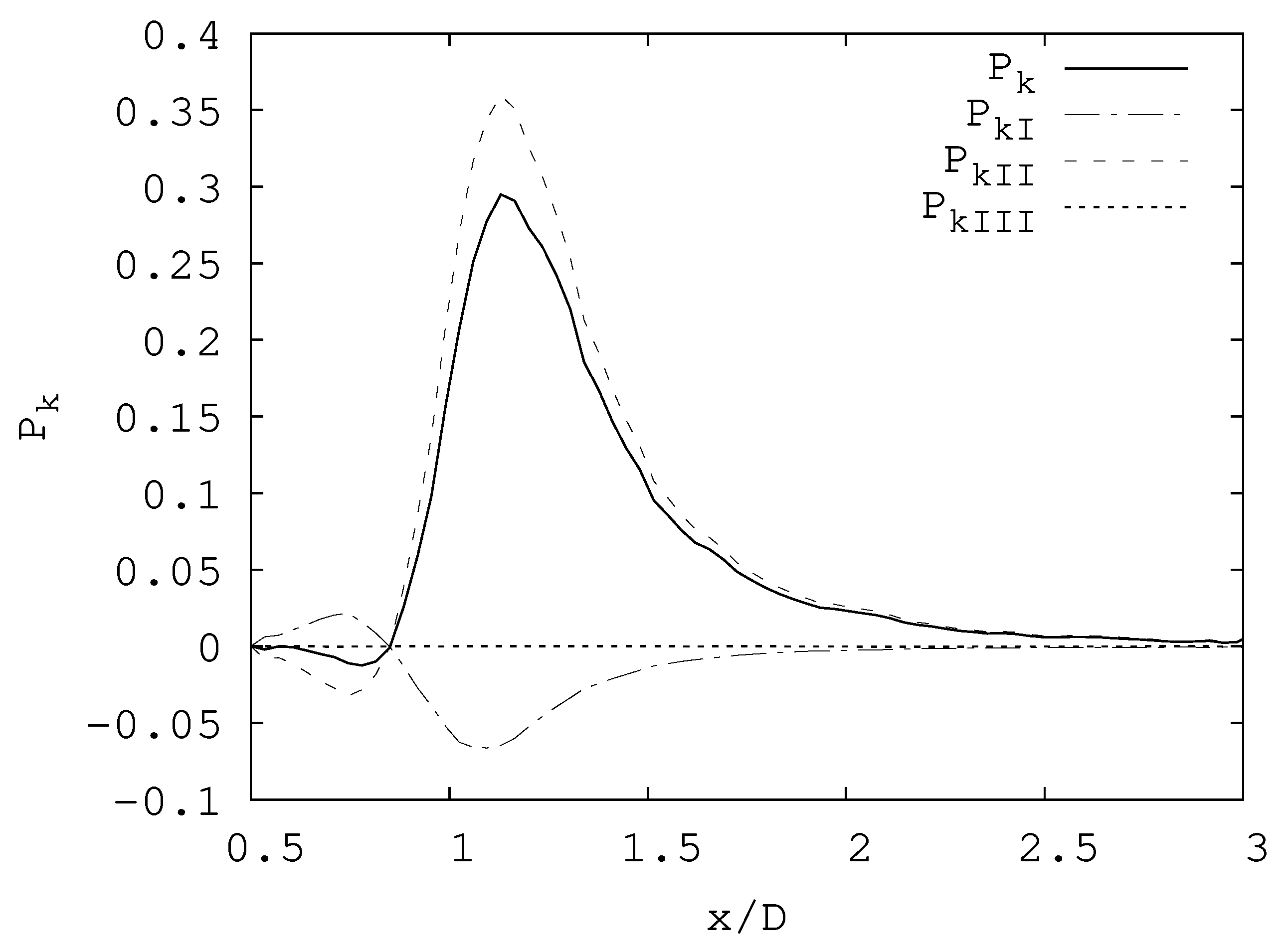
. If the contribution of the different terms to the production of the turbulent kinetic energy in the wake centerline is plotted (see Figure 10), one can readily observe that in the region where P k is negative, the first term in Equation (7) is positive and the second term is negative. The third term is zero, as u 1 u 2 ¯ is zero in the wake centerline. Considering this, Equation (6) can be re-written in the wake centerline as P k = ( u 1 u 1 ¯ u 2 u 2 ¯ ) u 1 x 1 . In other words, negative production in this zone is characterized by the domination of u 2 u 2 ¯ over u 1 u 1 ¯ .

3.3. Time–Frequency Analysis

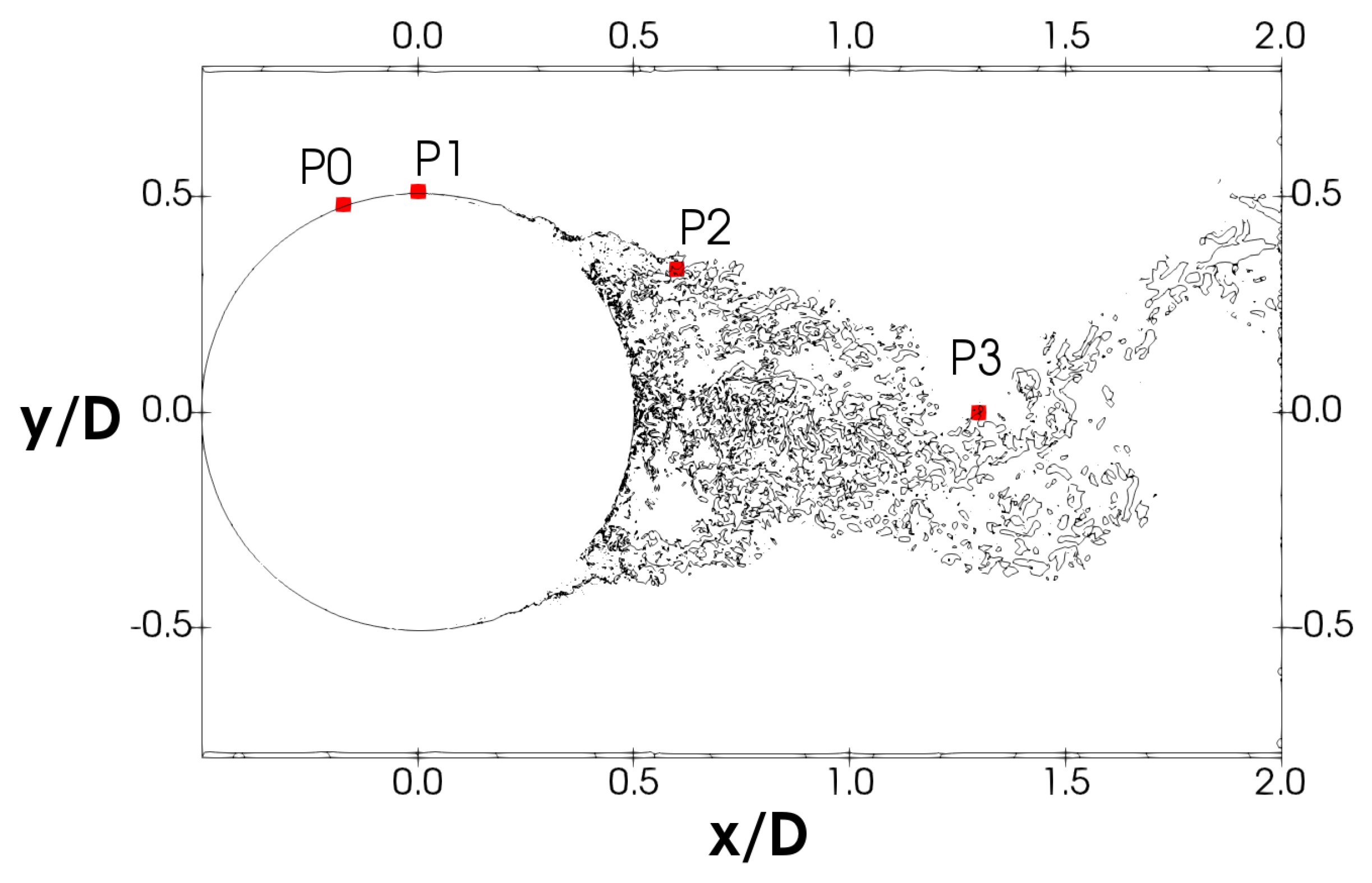
In order to determine the main frequencies of the flow, a set of different numerical probes is located in the boundary layer P 0 ( x 1 / D = 0.17 ;   x 2 / D = 0.47 ) and P 1 ( x 1 / D = 0 ;   x 2 / D = 0.5001 ) , the separated shear layer P 2 ( x 1 / D = 0.6 ;   x 2 / D = 0.33 ) and the wake P 3 ( x 1 / D = 1.3 ;   x 2 / D = 0 ) . In Figure 11, the location of these numerical probes in the ( x 1 x 2 ) plane is depicted. For each of these probes, the instantaneous signal of the flow is recorded at 128 stations in the homogeneous direction.
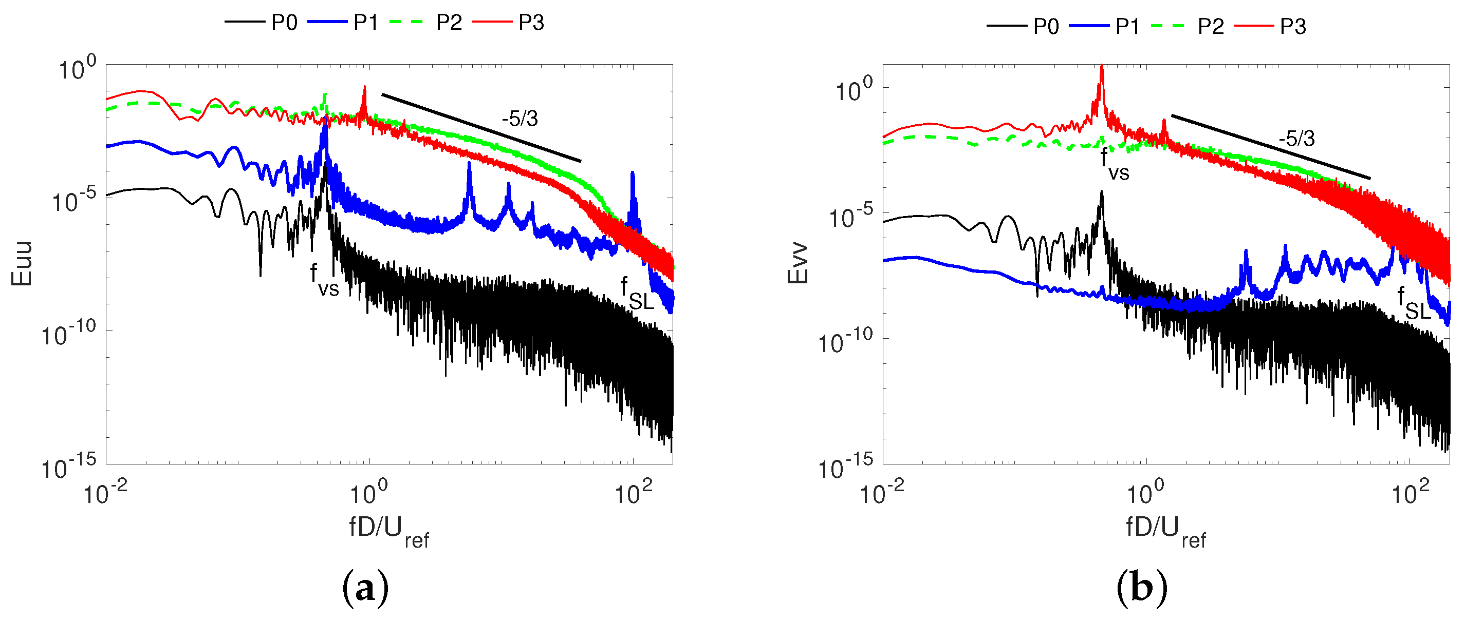
In Figure 12, the energy spectra of the stream-wise and cross-stream velocity fluctuations are plotted. As can be seen in the figure, different flow regimes are observed, from the laminar flow in the cylinder boundary layer (probe P 0 ), to the transitional flow (probe P 1 ) and the fully turbulent flow in the wake of the cylinder (probe P 3 ), where the energy spectrum exhibits the typical 5 / 3 slope in the inertial subrange. The spectra exhibit a pronounced peak at f D / U r e f = 0.458 , which can be identified with the large-scale vortex shedding frequency. As commented in Section 3.1, this value is in good agreement with those reported in the literature. The peak is detected by all the numerical probes, although its energy content might be different depending on the location of the probe. Notice also that for the probe located in the wake centerline, i.e., P 3 , due to the symmetry of the flow, the peak for the streamwise velocity fluctuations is located at twice the vortex shedding frequency.
In addition to the large-scale vortex shedding frequency, the energy spectrum at P 1 also detects a broad-band peak, whose maximum value is reached at the frequency f B L D / U r e f = 98.3 . Hereafter, this frequency is referred to as f B L , as the probe is located in the boundary layer (before the separation point). As will further be discussed, this peak is associated with the footprint of the transition to turbulence. In fact, it is only detected by the probe located in the cylinder shoulder. Downstream, in the probe located in the separated shear layer (i.e., probe P 2 ), it cannot be measured, as the flow in the shear layers is already turbulent.
The energy spectra showed in Figure 12 display more than one peak. In fact, one of the probes, P1, shows several frequency peaks and a very broadband frequency range. In order to separate the contributions to the energy spectrum of the boundary layer instabilities and the von Kármán vortices, a wavelet analysis is performed. Indeed, the wavelet analysis is capable of representing the temporal location of certain energetic events together with the spectral information of the signal.
The wavelet transform of a signal f ( t ) can be defined as follows:
W ( τ , b , f , ψ * ) = 1 τ f ( t ) ψ * t b τ d t
Here, ψ * is the generalized Morse wavelet [38], τ is the time scale, and b is the temporal translation. Considering that the term 1 / τ represents the frequency scale of an event and b its temporal location, W can be interpreted as the energetic content of the signal f at t = b , which occurs with a temporal scale τ . A comprehensive review on the wavelet transform and its application to turbulence flow can be found in the work of Farge [39].
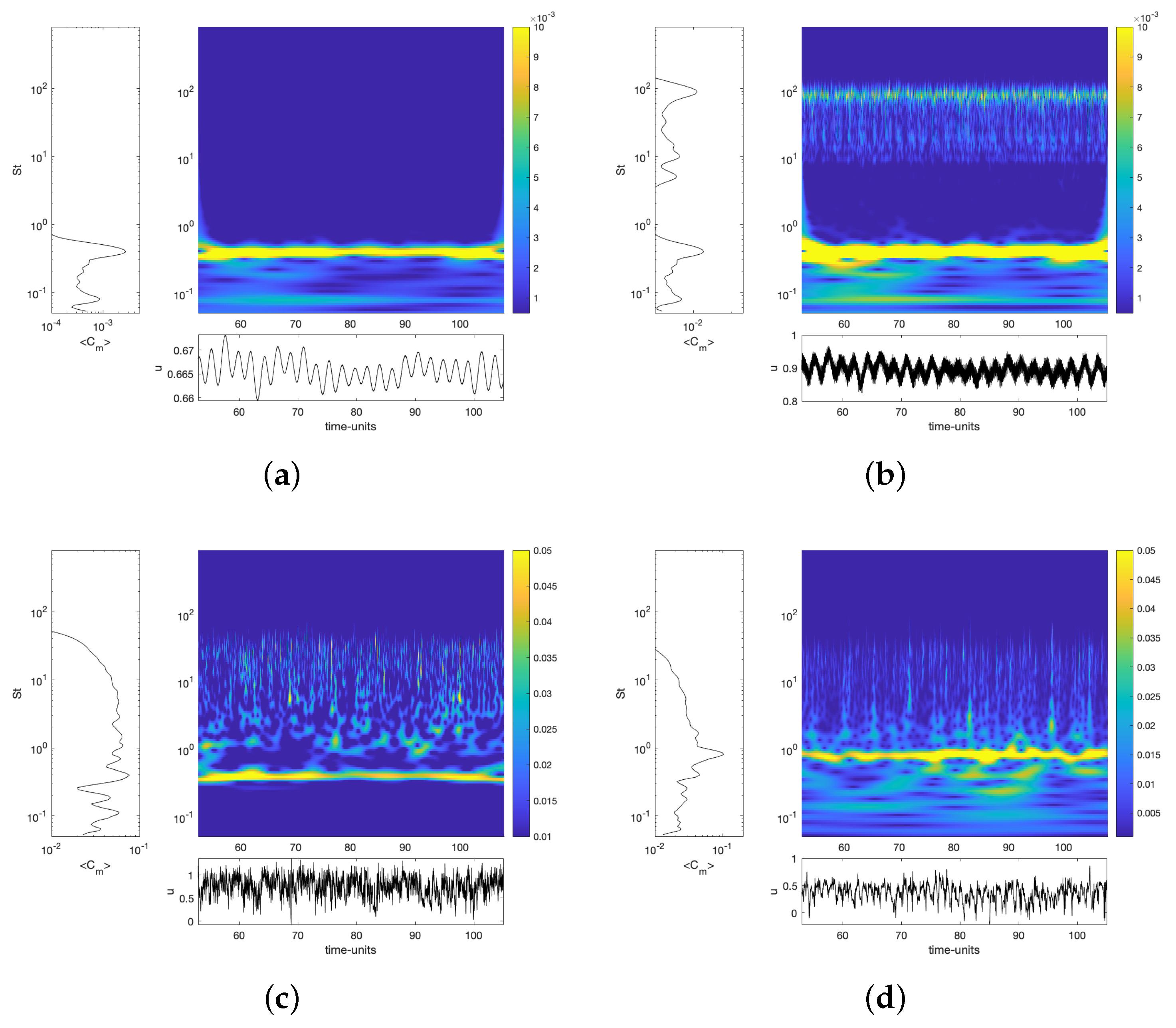
With this in mind, the wavelet analysis of the flow signals at different locations can be very useful to gain insight into the flow physics. In Figure 13, the time–frequency evolution of the modulus < C m > and the wavelet coefficient energy are plotted for the probes shown in Figure 11. The wavelet analysis shows a strong and coherent vortex shedding signal present at any time, captured at any location from the cylinder to the shear layers and the wake. The wavelet coefficient reaches a peak at the vortex shedding frequency. For the frequency associated with the transition to turbulence mechanism, it is centered at f B L D / U r e f = 88.9 , which is slightly smaller than the value that arises from the energy spectrum. Analyzing the signal, one can see that it is not constant in time but exhibits peaks of variable intensity, denoting also the instabilities that give rise to the transition to turbulence occurs intermittently along the spanwise location. This cannot be captured by the energy spectrum plotted in Figure 12. An interesting fact is that for the probe located in the detached shear layer, the wavelet coefficients do not show any particular signature at this high frequency, as the flow in this location of the shear layers is already turbulent and fluctuations due to instabilities are embedded into the turbulent fluctuations of the flow.
In Lehmkuhl et al. [6], the high frequency peak corresponding with boundary layer instabilities was related to the Kelvin–Helmholtz (KH) mechanism of transition to turbulence in the separated shear layers described by Bloor [40], the typical mechanism of transition in the sub-critical regime. However, instabilities here are triggered in the attached boundary layer and thus, they are not a KH type of instability. In the particular case of a boundary layer or a channel flow, Tollmien–Schlichting (TS) waves [41] are the primary instability mechanism of transition from laminar to turbulent flow. Boundary layers over curved surfaces are also prone to the growth of instabilities triggered by the action of centrifugal forces. In the case of concave surfaces, Görtler instabilities are known to occur, which are associated with a pair of counter-rotating streamwise vortices that become linearly unstable. Extensive reviews regarding this instability can be found in Hall [42] and Saric [43]. Although most of the studies have been focused on boundary layer instabilities in concave surfaces, Görtler instabilities over convex surfaces, as the case of the circular cylinder, were also recently studied [44,45]. However, whether instabilities here are of a TS type or are triggered by a centrifugal force deserve a more thorough analysis and is beyond the focus of the present study.

3.4. Phase-Averaged Flow

Interesting information about the wake topology can also be extracted from the study of the unsteady mean flow, which is here analyzed by means of the phase-average technique. The instantaneous flow can be represented by the contributions of a time-averaged quantity f i , a periodic fluctuation f i , and a random fluctuation f i [46], i.e., f i = f i + f i + f i . The phase average, defined as the average value of the variable f i over an ensemble of signals which have the same phase with respect to a reference signal, is f i ( ϕ ) ^ = f i + f i , ϕ being the phase angle, 0 ϕ 2 π .
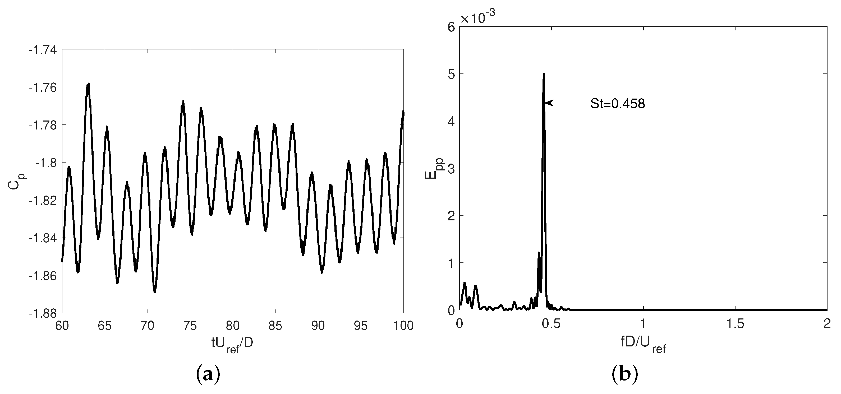
For the ensemble average, 10 vortex shedding cycles are used to generate each coherent component. Measurements of the phase-averaged quantities need a reference signal from which the phase of the flow is determined. In this case, the reference signal is obtained from a probe located in the front of the cylinder at 60 ° from the stagnation point (see Figure 14). In this region, the flow is more dominated by the periodic wave rather than by turbulent effects. The signal of the pressure coefficient exhibits clearly a strong periodic component, and it is not affected by the turbulence developed downstream. As can be seen from Figure 14b, the energy spectrum of the pressure coefficient fluctuations exhibits a dominant peak at the vortex shedding frequency f v s D / U r e f = 0.458 . Thus, the signal of the pressure coefficient is here used as a periodic oscillator. Following the period of the oscillator, the flow field is then classified according to its phase angle by dividing each period into windows of 2 π / 128 . However, due to the large storage capacity required for the 128 phase angles, only 8 of them were recorded (i.e., every π / 4 phase angle).
Distributions of the phase-averaged characteristics of the normal and shear Reynolds stresses for the sub-critical wake were provided by CC, Braza et al. [47] and Perrin et al. [48] at Reynolds number R e = 1.4 × 10 5 . In particular, CC investigated the contributions for the different components and pointed out the mechanisms of turbulent production and the role of the saddle points in the entrainment and turbulent production.
In 
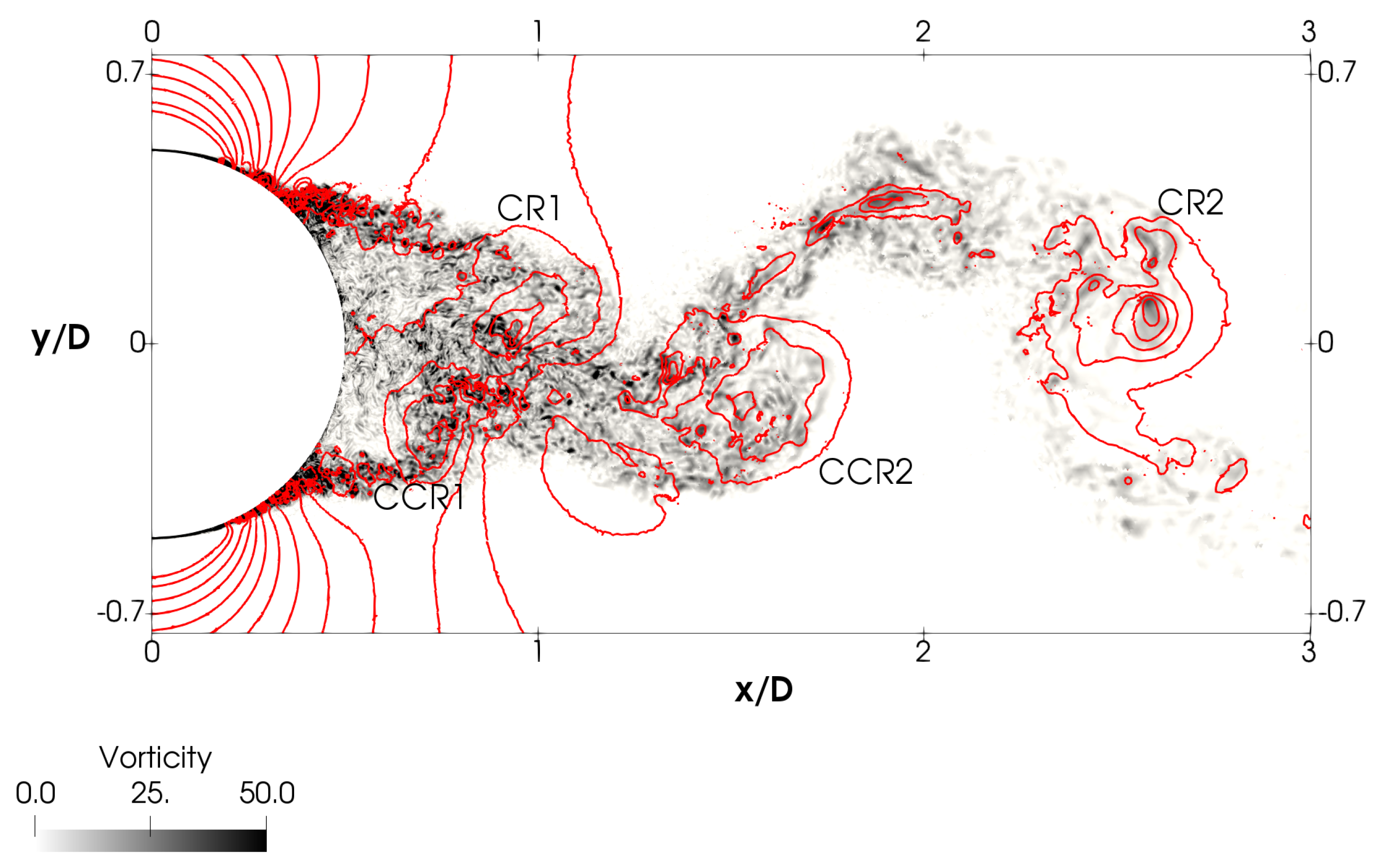
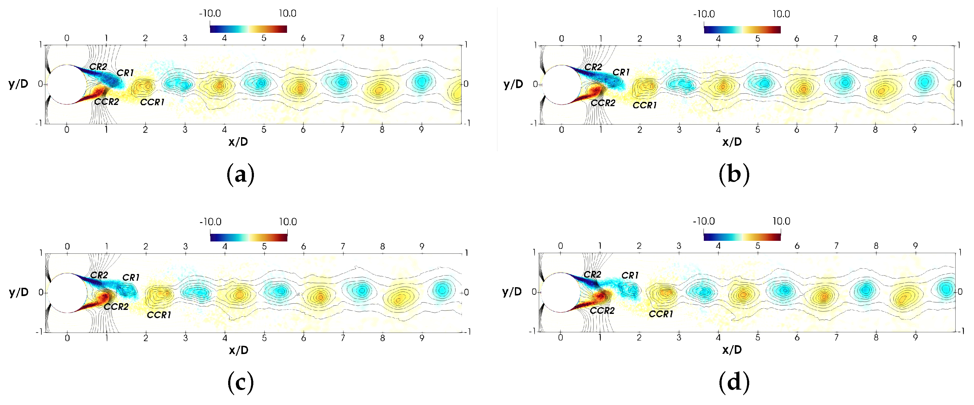
Figure 15, the streamlines at constant phase during half of the vortex shedding period are plotted. Additionally, in Figure 16, the phase-averaged vorticity and the pressure contours at constant phase are also given. Phase ϕ = 0 (see Figure 15a and Figure 16a) starts when the clockwise rotating vortex (CR1) is shed into the wake, and the lift coefficient has reached its maxima ( C L , m a x 0.074 ). A new vortex starts to be formed on the top shear layer (CR2), whereas the counter-clockwise rotating vortex (CCR2) in the bottom shear layer steadily rolls up and grows from phase ϕ = 0 to ϕ = 2 π / 3 . The location of the saddle point moves downstream and toward the wake centerline as CR2 develops. The half vortex shedding period ends when CCR2 is about to be shed into the wake and the lift coefficient reaches its minima ( C L , m i n 0.074 ).
Vorticity peaks at the center of the vortices, as can be seen in Figure 16, but its magnitude decreases as the vortices move downstream from the shear layers to the wake. In the vortex formation region, the non-dimensional spanwise vorticity maximum is around | ω 3 | = 9.5 to | ω 3 | = 7.5 as the vortices move from x 1 / D = 0.85 to x 1 / D = 1.33 at the outer limit of the recirculation region. This is in contrast with the values reported in the sub-critical regime by Braza et al. [47], who observed absolute vorticity to decrease from 3 to 1 as the vortex moves toward the closure of the vortex formation zone. In the wake centerline, the absolute magnitude of spanwise vorticity at the vortex cores diminishes and ranges around | ω 3 | = 2.9 4 (see Figure 16).
After being shed, in the sub-critical wake, vortices travel almost parallel to the wake axis. CC reported that centroids were at x 2 / D = 0.35 from the wake centerline, whereas Braza et al. [47] measured a distance of Δ x 2 / D = 0.25 . In the super-critical wake, vortices travel downstream almost at the wake centerline. The distance from the wake centerline to the vortex center is, on average, Δ x 2 / D 0.022 , with their centroids separated each other about Δ x 1 / D = 2.05 . This value was reported to be twice the distance in the sub-critical regime ( Δ x 1 / D = 4.3 ) by CC, as vortex shedding frequency is half the value measured in the super-critical regime.
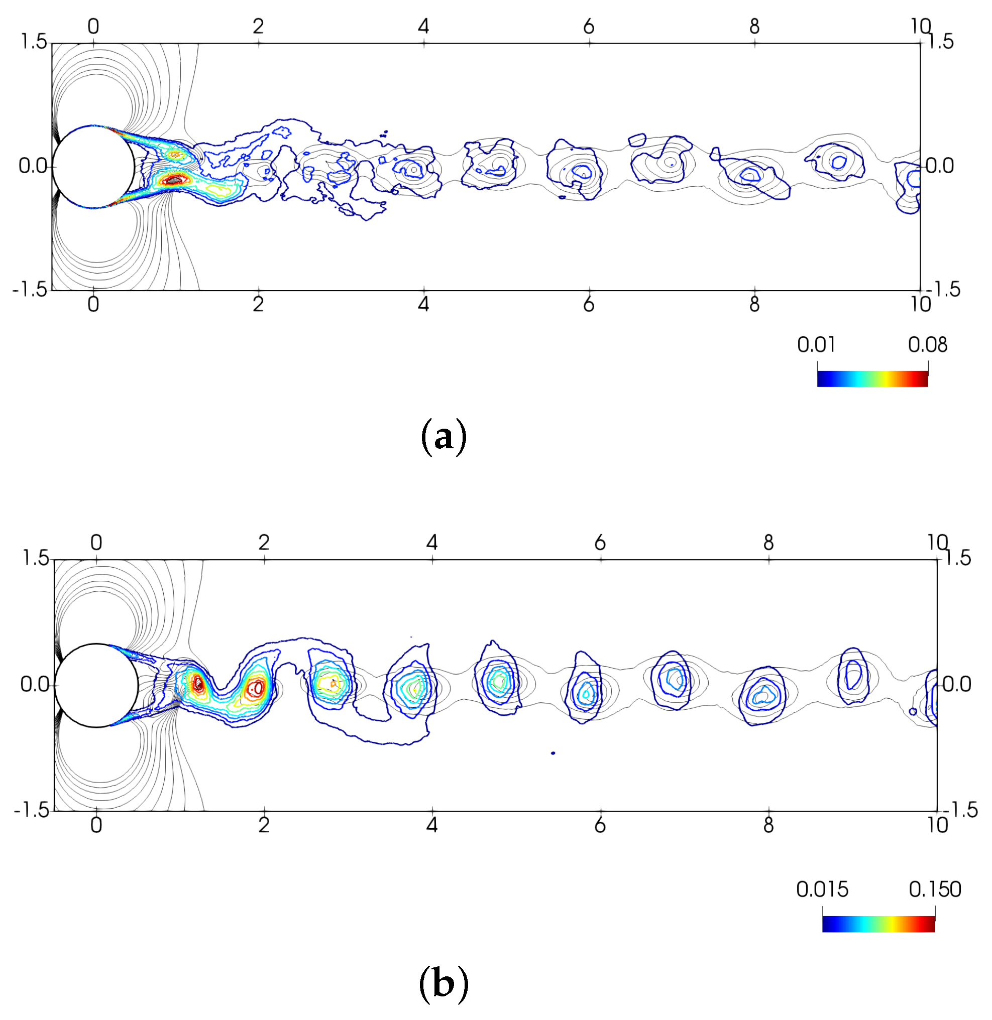
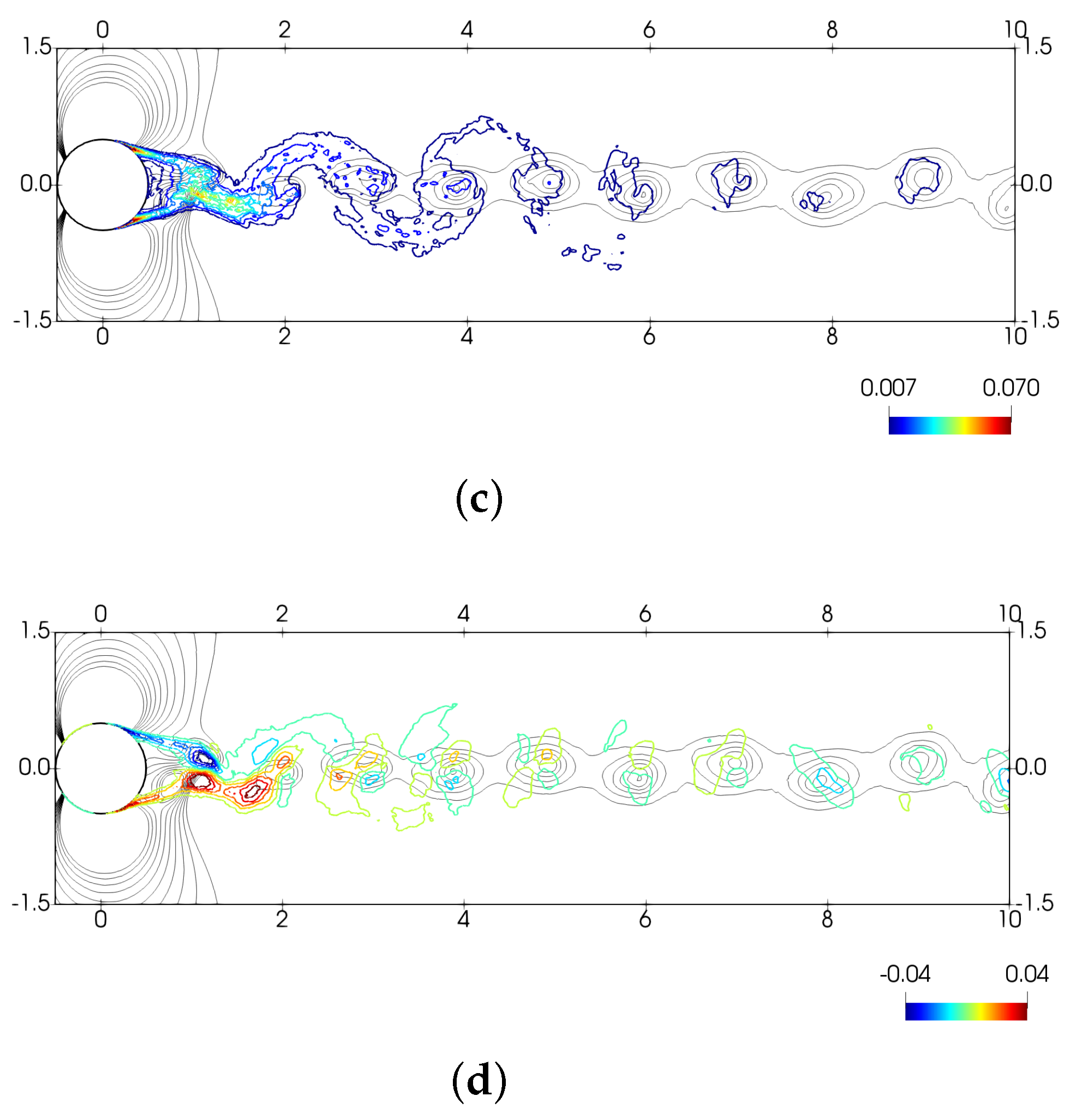
The Reynolds stresses at constant phase are evaluated and shown for phase ϕ = 0 in Figure 17. Random normal Reynolds stresses are concentrated in the regions of high vorticity, i.e., at the vortex cores. Overall, random maximum values of the Reynolds stresses are observed in the vortex formation zone. For the streamwise normal stresses, u 1 u 1 / U r e f 2 , these extrema are located at the core of the forming vortex, whereas for u 2 u 2 / U r e f 2 they are located nearby the closure of the vortex formation zone. In the wake, normal Reynolds stresses maxima are located at the vortex cores, whereas the shear stresses maximum is in the region between vortices. It is observed that the peak value for u 1 u 1 / U r e f 2 is around 0.08. As vortices move downstream into the wake, the peak registered at the vortex center decreases; it is about u 1 u 1 / U r e f 2 0.025 at x 1 / D = 5 . The value reported by CC for the sub-critical wake is about u 1 u 1 / U r e f 2 0.0935 , which is almost 4 times larger. Differences can be attributed to both the location of the separation point from the cylinder and the state of the boundary layer at separation. In fact, the values here reported are in fair agreement with those obtained by Rai [49] for a flat plate with turbulent separation. For u 2 u 2 / U r e f 2 (see Figure 17b), the peak value in the vortex formation zone is about 0.165, and at the normal streamwise Reynolds stress, the magnitude of the peak at the vortex cores decreases steadily; at x 1 / D = 5 , it is about u 2 u 2 / U r e f 2 0.08 .

4. Summary

Large eddy simulations of the flow past a circular cylinder at the super-critical Reynolds number of R e = 7.2 × 10 5 were performed, using a low-dissipation FEM code. The characteristics of the wake topology were studied and described in detail. At this Reynolds number, the onset of instabilities occurs in the attached boundary layer and eventually triggers the transition to turbulence. The energy spectra and wavelet analysis show that the inception of boundary layer instabilities is not constant in time, but exhibits peaks of variable energy and occurs at a frequency of f B L D / U r e f = 88.9 . After transition to turbulence, the boundary layer detaches from the rear side of the cylinder surface at ϕ s = 149 .
Due to the delayed separation, the recirculation region behind the cylinder is restricted to a small zone, which extends up to x 1 / D = 1.07 . The near wake topology is shown to be symmetrical with the typical two-lobed pattern, similar to the one observed in the subcritical regime. However, due to the inclination of the shear layers towards the wake centerline, strong cross-stream velocity gradients are observed in the shear layers, a trait that is not observed in the sub-critical regime. Turbulent kinetic energy and Reynolds stresses have also a different behavior. While in the sub-critical regime, maximum values are attained in the vortex formation region, close to the closure of the recirculation, in the super-critical wake, highest values are registered along the shear layers close to the separation of the turbulent boundary layer. The analysis has shown that the largest values come from the turbulent production in the zone, the major contribution being from the cross-streamwise normal stresses. Moreover, in the vortex formation region, the magnitude of the peak in the stresses is lower than in the sub-critical regime, owing to the narrower wake and lower contribution of the coherent component. A region of negative production in the wake centerline, related to the larger contribution of the cross-stream Reynolds stresses was also reported to occur at x 1 / D = 0.8 . Last but not least, the analysis of the unsteady mean flow has shown that contrary to the sub-critical regime, where vortexes formed travel down parallel to the wake centerline, in the super-critical regime, these vortexes travel almost following the wake centerline, with the streamwise distance being half of that measured in the sub-critical regime.

Author Contributions

Conceptualization, I.R. and O.L.; methodology, I.R. and O.L.; software, O.L.; validation, I.R.; formal analysis, I.R.; investigation, I.R. and O.L; writing—original draft preparation, I.R.; writing—review and editing, I.R. and O.L. All authors have read and agreed to the published version of the manuscript. On the characteristics of the super-critical wake behind a circular cylinder.

Funding

This work was partially financially supported by the Ministerio de Economía y Competitividad, Secretaría de Estado de Investigación, Desarrollo e Innovación, Spain (Ref. TRA2017-88508-R) and by European Union’s Horizon 2020 research and innovation programme (INFRAEDI-02-2018, EXCELLERAT- The European Centre Of Excellence For Engineering Applications H2020). The work of O. Lehmkuhl is financed by a Ramón y Cajal postdoctoral contract by the Ministerio de Economía y Competitividad, Secretaría de Estado de Investigación, Desarrollo e Innovación, Spain (RYC2018-025949-I)).

Institutional Review Board Statement

Not applicable.

Informed Consent Statement

Not applicable.

Acknowledgments

We also acknowledge PRACE for awarding us access to SuperMUC supercomputer (Project ViValdi Ref. 2017174222).

Conflicts of Interest

The authors declare no conflict of interest.

Appendix A. Mesh Verification Studies

In a wall-resolved LES, it must be ensured that the computational grid used has enough resolution and the viscous boundary layer is well resolved and away the wall; the mesh can solve most of the inertial sub-range. The former can be enforced by computing the boundary layer thickness and ensuring that at least 8–10 grid points are within the boundary layer. Moreover, the distance to the first off-wall element should be kept y n + < 2 [50]. In this work, these two conditions are verified for the computational mesh in the near wall region. The latter, i.e., the mesh density in the off-the-wall regions, can be verified by computing the ratio of the mesh size to the Kolmogorov scale ( h / η ).
In Figure A1, the ratio of the grid size to the Kolmogorov length scale at different locations in the wake behind the cylinder is plotted. Here, the grid size is computed as h = Ω 1 / 3 , with Ω being the cell volume. The Kolmogorov length scale η = ( ν 3 / η ) 1 / 4 is evaluated by computing the dissipation rate ϵ as ϵ = 2 ( ν + ν s g s ) S i j S i j ¯ , where S i j ¯ is the mean rate-of-strain fluctuations. As can be seen from the figure, in the near wake, up to x 1 / D 5 the ratio h / η is kept lower than 10 ( h / η < 10 ) and it increases up to h / η 18 at x 1 / D = 8 . According to Pope [51], the scales responsible for the dissipation are in the range 8 / η 60 , with the peak on the dissipation spectrum at / η = 24 . Thus, on this basis, the mesh used for the present computations should be enough for covering most of the energy cascade and performing LES of the flow.
Figure A1. Ratio of the grid size to the Kolmogorov length scale ( h / η ) at different locations in the near wake.
Fluids 06 00396 g0a1

References

  1. Roshko, A. On the Development of Turbulent Wakes from Vortex Streets; Technical Report NACA TR 1191; California Institute of Technology: Pasadena, CA, USA, 1954. [Google Scholar]
  2. Roshko, A. Perspectives on Bluff Body Wakes. J. Wind. Eng. Ind. Aerodyn. 1993, 49, 79–100. [Google Scholar] [CrossRef]
  3. Achenbach, E. Distribution of local pressure and skin friction around a circular cylinder in cross-flow up to Re = 5×10⁶. J. Fluid Mech. 1968, 34, 625–639. [Google Scholar] [CrossRef]
  4. Bearman, P.W. On vortex shedding from a circular cylinder in the critical Reynolds number regime. J. Fluid Mech. 1969, 37, 577–585. [Google Scholar] [CrossRef]
  5. Shih, W.; Wang, C.; Coles, D.; Roshko, A. Experiments on flow past rough circular cylinders at large Reynolds numbers. J. Wind. Eng. Ind. Aerodyn. 1993, 49, 351–368. [Google Scholar] [CrossRef]
  6. Lehmkuhl, O.; Rodríguez, I.; Borrell, R.; Chiva, J.; Oliva, A. Unsteady forces on a circular cylinder at critical Reynolds numbers. Phys. Fluids 2014, 26, 125110. [Google Scholar] [CrossRef] [Green Version]
  7. Yeon, S.M.; Yang, J.; Stern, F. Large eddy simulation of the flow past a circular cylinder at sub- to super-critical Reynolds numbers. Appl. Ocean. Res. 2016, 59, 663–675. [Google Scholar] [CrossRef] [Green Version]
  8. Cheng, W.; Pullin, D.I.; Samtaney, R.; Zhang, W.; Gao, W. Large-eddy simulation of flow over a cylinder with ReD from 3.9 × 10³ to 8.5 × 10⁵: A skin-friction perspective. J. Fluid Mech. 2017, 820, 121–158. [Google Scholar] [CrossRef]
  9. Ahmadi, M.H.; Yang, Z. Large eddy simulation of the flow past a circular cylinder at super-critical reynolds numbers. Proc. Asme Turbo Expo 2020, 2C-2020, 663–675. [Google Scholar] [CrossRef]
  10. Cantwell, B.; Coles, D. An experimental study of entrainment and transport in the turbulent near wake of a circular cylinder. J. Fluid Mech. 1983, 136, 321–374. [Google Scholar] [CrossRef] [Green Version]
  11. Unal, M.F.; Rockwell, D. On vortex formation from a cylinder. Part 1. The initial instability. J. Fluid Mech. 1988, 190, 491–512. [Google Scholar] [CrossRef]
  12. Norberg, C. LDV measurements in the near wake of a circular cylinder. In Proceedings of the ASME Conference on Advances in the Understanding of Bluff Body Wakes and Vortex Induced Vibration, Washington, DC, USA, 1 June 1998. [Google Scholar]
  13. Ma, X.; Karamanos, G.; Karniadakis, G. Dynamics and low-dimensionality of a turbulent wake. J. Fluid Mech. 2000, 410, 29–65. [Google Scholar] [CrossRef] [Green Version]
  14. Dong, S.; Karniadakis, G.E.; Ekmekci, A.; Rockwell, D. A combined direct numerical simulation-particle image velocimetry study of the turbulent near wake. J. Fluid Mech. 2006, 569, 185. [Google Scholar] [CrossRef] [Green Version]
  15. Lehmkuhl, O.; Rodríguez, I.; Borrell, R.; Oliva, A. Low-frequency unsteadiness in the vortex formation region of a circular cylinder. Phys. Fluids 2013, 25, 085109. [Google Scholar] [CrossRef] [Green Version]
  16. Rodríguez, I.; Lehmkuhl, O.; Chiva, J.; Borrell, R.; Oliva, A. On the flow past a circular cylinder from critical to super-critical Reynolds numbers: Wake topology and vortex shedding. Int. J. Heat Fluid Flow 2015. [Google Scholar] [CrossRef] [Green Version]
  17. Schewe, G. On the force fluctuations acting on a circular cylinder in crossflow from subcritical up to transcritical Reynolds numbers. J. Fluid Mech. 1983, 133, 265–285. [Google Scholar] [CrossRef]
  18. Roshko, A. Experiments on the flow past a circular cylinder at very high Reynolds number. J. Fluid Mech. 1961, 10, 345–356. [Google Scholar] [CrossRef] [Green Version]
  19. Zdravkovich, M.M. Conceptual Overview of Laminar and Turbulent Flows Past Smooth and Rough Circular Cylinders. J. Wind. Eng. Ind. Aerodyn. 1990, 33, 53–62. [Google Scholar] [CrossRef]
  20. Vreman, A.W. An eddy-viscosity subgrid-scale model for turbulent shear flow: Algebraic theory and applications. Phys. Fluids 2004, 16, 3670–3681. [Google Scholar] [CrossRef]
  21. Vázquez, M.; Houzeaux, G.; Koric, S.; Artigues, A.; Aguado-Sierra, J.; Arís, R.; Mira, D.; Calmet, H.; Cucchietti, F.; Owen, H.; et al. Alya: Multiphysics engineering simulation toward exascale. J. Comput. Sci. 2016, 14, 15–27. [Google Scholar] [CrossRef] [Green Version]
  22. Lehmkuhl, O.; Houzeaux, G.; Owen, H.; Chrysokentis, G.; Rodriguez, I. A low-dissipation finite element scheme for scale resolving simulations of turbulent flows. J. Comput. Phys. 2019, 390, 51–65. [Google Scholar] [CrossRef]
  23. Capuano, F.; Coppola, G.; Rández, L.; de Luca, L. Explicit Runge-Kutta schemes for incompressible flow with improved energy-conservation properties. J. Comput. Phys. 2017, 328, 86–94. [Google Scholar] [CrossRef]
  24. Trias, F.X.; Lehmkuhl, O. A self-adaptive strategy for the time integration of Navier-Stokes equations. Numer. Heat Transf. Part B 2011, 60, 116–134. [Google Scholar] [CrossRef]
  25. Pastrana, D.; Cajas, J.C.; Lehmkuhl, O.; Rodríguez, I.; Houzeaux, G. Large-eddy simulations of the vortex-induced vibration of a low mass ratio two-degree-of-freedom circular cylinder at subcritical Reynolds numbers. Comput. Fluids 2018, 173, 118–132. [Google Scholar] [CrossRef] [Green Version]
  26. Rodriguez, I.; Lehmkuhl, O.; Soria, M.; Gomez, S.; Domınguez-Pumar, M.; Kowalski, L. Fluid dynamics and heat transfer in the wake of a sphere. Int. J. Heat Fluid Flow 2019, 76, 141–153. [Google Scholar] [CrossRef]
  27. Rodriguez, I.; Lehmkuhl, O.; Borrell, R. Effects of the actuation on the boundary layer of an airfoil at Reynolds number Re = 60000. Flow Turbul. Combust. 2020, 390, 51–65. [Google Scholar] [CrossRef]
  28. Rodriguez, I.; Lehmkuhl, O.; Soria, M. On the effects of the free-stream turbulence on the heat transfer from a sphere. Int. J. Heat Mass Transf. 2021, 164, 120579. [Google Scholar] [CrossRef]
  29. Schewe, G. Sensitivity of transition phenomena to small perturbations in flow round a circular cylinder. J. Fluid Mech. 1986, 172, 33–46. [Google Scholar] [CrossRef]
  30. Jeong, J.; Hussain, F. On the identification of a vortex. J. Fluids Mech. 1995, 285. [Google Scholar] [CrossRef]
  31. Achenbach, E.; Heinecke, E. On vortex shedding from smooth and rough cylinders in the range of Reynolds numbers 6e3 to 5e6. J. Fluid Mech. 1981, 109, 239–251. [Google Scholar] [CrossRef]
  32. Williamson, C.H.K. Vortex dynamics in the cylinder wake. Annu. Rev. Fluid Mech. 1996, 28, 477–539. [Google Scholar] [CrossRef]
  33. Spitzer, R. Measurements of Unsteady Pressures and Wake Fluctuations for Flow over a Cylinder at Supercritical Reynolds Number. Ph.D. Thesis, California Institute of Technology, Pasadena, CA, USA, 1965. [Google Scholar]
  34. Aljure, D.E.; Rodríguez, I.; Lehmkuhl, O.; Pérez-Segarra, C.D.; Oliva, A. Influence of rotation on the flow over a cylinder at Re = 5000. Int. J. Heat Fluid Flow 2015, 55, 76–90. [Google Scholar] [CrossRef] [Green Version]
  35. Tani, I. Low-speed flows involving bubble separations. Prog. Aerosp. Sci. 1964, 5, 70–103. [Google Scholar] [CrossRef]
  36. Palkin, E.; Mullyadzhanov, R.; Hadžiabdić, M.; Hanjalić, K. Scrutinizing URANS in Shedding Flows: The Case of Cylinder in Cross-Flow in the Subcritical Regime. Flow Turbul. Combust. 2016, 97, 1017–1046. [Google Scholar] [CrossRef]
  37. Rodriguez, I.; Lehmkuhl, O.; Piomelli, U.; Chiva, J.; Borrell, R.; Oliva, A. LES-based Study of the Roughness Effects on the Wake of a Circular Cylinder from Subcritical to Transcritical Reynolds Numbers. Flow Turbul. Combust. 2017, 99, 729–763. [Google Scholar] [CrossRef]
  38. Olhede, S.C.; Walden, A.T. Generalized Morse wavelets. IEEE Trans. Signal Process. 2002, 50, 2661–2670. [Google Scholar] [CrossRef] [Green Version]
  39. Farge, M. Wavelet transforms and their applications to turbulence. Annu. Rev. Fluid Mech. 1992, 24, 395–457. [Google Scholar] [CrossRef]
  40. Bloor, M. The transition to turbulence in the wake of a circular cylinder. J. Fluid Mech. 1964, 19, 290–304. [Google Scholar] [CrossRef]
  41. Klebanoff, P.S.; Tidstrom, K.D.; Sargent, L.M. The three-dimensional nature of boundary-layer instability. J. Fluid Mech. 1962, 12, 1–34. [Google Scholar] [CrossRef] [Green Version]
  42. Hall, P. On the stability of the unsteady boundary layer on a cylinder oscillating transversely in a viscous fluid. J. Fluid Mech. 1984, 146, 347–367. [Google Scholar] [CrossRef] [Green Version]
  43. Saric, W.S. Gortler vortices. Annu. Rev. Fluid Mech. 1994, 26, 379–409. [Google Scholar] [CrossRef]
  44. Karp, M.; Hack, P. Transition to turbulence over convex surfaces. J. Fluid Mech. 2018, 855, 1208–1237. [Google Scholar] [CrossRef]
  45. Pastrana, D.; Rodriguez, I.; Cajas, J.; Lehmkuhl, O.; Houzeaux, G. On the formation of Taylor-Görtler structures in the vortex induced vibration phenomenon. Int. J. Heat Fluid Flow 2020, 83, 108573. [Google Scholar] [CrossRef]
  46. Reynolds, W.C.; Hussain, A.K.M.F. The mechanics of an organized wave in turbulent shear flow. Part 3. Theoretical models and comparisons with experiments. J. Fluid Mech. 1972, 54, 263–288. [Google Scholar] [CrossRef]
  47. Braza, M.; Perrin, R.; Hoarau, Y. Turbulence properties in the cylinder wake at high Reynolds numbers. J. Fluids Struct. 2006, 22, 757–771. [Google Scholar] [CrossRef] [Green Version]
  48. Perrin, R.; Cid, E.; Cazin, S.; Sevrain, A.; Braza, M.; Moradei, F.; Harran, G. Phase-averaged measurements of the turbulence properties in the near wake of a circular cylinder at high Reynolds number by 2C-PIV and 3C-PIV. Exp. Fluids 2007, 42, 93–109. [Google Scholar] [CrossRef]
  49. Rai, M.M. Flow physics in the turbulent near wake of a flat plate. J. Fluid Mech. 2013, 724, 704–733. [Google Scholar] [CrossRef]
  50. Piomelli, U.; Chasnov, J.R. Transition and Turbulence Modelling; Chapter Large-eddy Simulations and Applications; Kluwer Academic Publishers: Dordrecht, The Netherlands, 1996; pp. 269–331. [Google Scholar]
  51. Pope, S. Turbulent Flows; Cambridge University Press: Cambridge, UK, 2000. [Google Scholar]
Figure 1. Vortical structures identified by means of Q iso-contours colored by the velocity magnitude.
Fluids 06 00396 g001
Figure 2. Instantaneous wake: pressure coefficient iso-contours.
Fluids 06 00396 g002
Figure 3. Instantaneous vorticity magnitude superimposed with pressure coefficient iso-contours (red) in the vortex formation zone.
Fluids 06 00396 g003
Figure 4. (a) Pressure coefficient and (b) skin-friction distribution along the cylinder surface. Comparison with the literature. SPI65 (Spitzer [33]), FLA29 (Flachbart experiments taken from [18]), CHE17 (Cheng et al. [8]), ACH68 (Achenbach [3]).
Fluids 06 00396 g004
Figure 5. Mean wake recirculation zone scheme (a) sub-critical regime, (b) super-critical regime.
Fluids 06 00396 g005
Figure 6. (a) Stream-wise velocity and (b) its fluctuations in the wake centerline. Comparison with sub-critical and super-critical results. The red solid line present the results; (black dash-dot line) R e = 7.2 × 10 5 [16]; (blue line) R e = 3900 [15]; (purple circles) R e = 5000 [34]; (green squares) R e = 1.4 × 10 5 [10].
Fluids 06 00396 g006
Figure 7. Near wake mean field. (a) Streamlines; non-dimensional iso-contours of (b) pressure coefficient ( 2.2 C p 1 : 0.36 ); (c) stream-wise velocity ( 0.25 u 1 / U r e f 1.8 : 0.205 ); (d) cross-stream velocity ( 0.9 u 2 / U r e f 0.9 : 0.2 ).
Fluids 06 00396 g007
Figure 8. Second order turbulent statistics. (a) Stream-wise normal stresses u 1 u 1 ¯ / U r e f 2 , (b) cross-stream wise normal u 2 u 2 ¯ / U r e f 2 , (c) shear stresses u 1 u 2 ¯ / U r e f 2 , (d) turbulent kinetic energy k / U r e f 2 .
Fluids 06 00396 g008
Figure 9. (a) Mean turbulent kinetic energy production P k . (bd) Production for the normal and shear stresses u 1 u 1 / U r e f 2 , u 2 u 2 / U r e f 2 and u 1 u 2 / U r e f 2 . (b) P 11 , (c) P 22 , (d) P 12 .
Fluids 06 00396 g009
Figure 10. Production of turbulent kinetic energy in the wake centerline and the contribution of the different terms in Equations in Section 3.1.
Fluids 06 00396 g010
Figure 11. Location of the numerical probes.
Fluids 06 00396 g011
Figure 12. Energy spectra at different locations. (a) for stream-wise velocity fluctuations, (b) for cross-stream wise velocity fluctuations.
Fluids 06 00396 g012
Figure 13. {Time–frequency} analysis using the continuous wavelet transform of the streamwise velocity component at different locations. (a) Cylinder boundary layer at 70 ° from the front stagnation point; (b) cylinder boundary layer at 90 ° from the front stagnation point; (c) in the separated shear layer at ( x / D , y / D ) ( 0.6 , 0.33 ) ; (d) at the wake centerline at ( x / D , y / D ) ( 1.3 , 0 ) .
Fluids 06 00396 g013
Figure 14. (a) Reference signal used as periodic oscillator. (b) Power spectrum of the reference oscillator signal.
Fluids 06 00396 g014
Figure 15. Phase-averaged streamlines. (a) ϕ = 0 , (b) ϕ = π / 4 , (c) ϕ = π / 2 , (d) ϕ = 3 π / 4 . The location of the saddle point is also marked.
Fluids 06 00396 g015
Figure 16. Phase averaged spanwise vorticity superimposed with pressure contours in the wake at constant phase. (a) ϕ = 0 , (b) ϕ = π / 4 , (c) ϕ = π / 2 , (d) ϕ = 3 π / 4 .
Fluids 06 00396 g016
Figure 17. Contours of the random component of the normal and shear stresses at constant phase, ϕ = 0 , plotted over pressure coefficient contours (in black) (a) u 1 u 1 / U r e f 2 , (b) u 2 u 2 / U r e f 2 , (c) u 3 u 3 / U r e f 2 , (d) u 1 u 2 / U r e f 2 .
Fluids 06 00396 g017aFluids 06 00396 g017b
Table 1. Statistics in the near-wake: maximum normal and shear Reynolds stresses u 1 u 1 / U r e f 2 , u 2 u 2 / U r e f 2 , u 1 u 2 / U r e f 2 , maximum turbulent kinetic energy k / U r e f 2 and minimum stream-wise velocity in the wake centerline. The positions of these extrema are also given. † [10], ‡ [34], § [15].
Re
7 . 2 × 10 5 1.4 × 10 5 5000 3900 §
u 1 u 1 m a x / U r e f 2 0.1020.220.2390.237
( x 1 / D , x 2 / D ) (1.033, ±0.149) (1.587, ±0.297)(1.576, ±0.310)
u 2 u 2 m a x / U r e f 2 0.2010.430.4670.468
( x 1 / D , x 2 / D ) (1.216, 0) (1.992, 0)(2.000, 0)
u 1 u 2 m i n / U r e f 2 ±0.06±0.19±0.128±0.125
( x 1 / D , x 2 / D ) (1.161, ±0.138) (1.901, ±0.422)(1.941, ±0.391)
k m a x / U r e f 2 0.138-0.3310.335
( x 1 / D , x 2 / D ) (1.106, ±0.109) (1.764, ±0.202)(1.775, ±0.216)
u 1 m i n / U r e f −0.255-−0.284−0.261
( x 1 / D , x 2 / D ) (0.845, 0) (1.399, 0)(1.396, 0)
Publisher’s Note: MDPI stays neutral with regard to jurisdictional claims in published maps and institutional affiliations.

