1. Introduction
Electroless plating is an industrial chemical process aimed at forming a thin film or layer on a base substrate by reducing complex metal cations in a liquid solution [
1,
2,
3]. This technique has been widely applied in various industries. For instance, surface decoration, hard-wearing coating, manufacture of hard-disc drive, printed circuit boards, etc. [
3,
4]. It is well known that many electroless plating processes produce parasite hydrogen bubbles, such as electroless nickel and electroless copper systems [
5,
6,
7]. There are several works on the simulation of electroless processes that study the convection or migration of chemical species under a single-phase flow (e.g., [
8,
9]). As far as we know, there is no computational work on bubble generation in an electroless process. In large-scale electroless plating processes, the gas generation will not be a serious issue, in general, however, for micro-scale plating, hydrogen bubbles may prevent electrolytes from going into the region needed to be plated. The existence of relatively large bubbles has been an important issue in the study of micro-fluids [
10,
11,
12]. As experiments are difficult, there is a need for a reliable numerical simulation tool.
From a theoretical physics point of view, electroless processes are complex; the entire physical system participates to the plating. Therefore, for the simulation, we chose a system that includes a gas–liquid two-phase flow, chemical species transport, surface reaction, and moving boundary due to deposition.
1.1. The Modeling
Because bubbles and sprays are frequent in engineering design with fluids, numerous papers on the modeling and simulation of gas–liquid two-phase flows have been published such as [
13,
14,
15,
16,
17]. Working models to compute gas–fluid flows can be sorted into two classes: (i) phase field or level set models where the gas–liquid interface is traced [
18,
19,
20,
21]; (ii) averaged models [
22,
23,
24]. Several reasons support our choice for an averaged model: (i) There are many bubbles and their generation seems random, we only know that there is a higher chance of gas generation occurring in regions of higher concentration of dissolved gas; (ii) even if the bubble generation can be well predicted, vast amounts of bubbles are generated in short moments and the computational cost for capturing each bubble is prohibitive; (iii) interfacial terms (e.g., terms caused by a phase change) can be easily estimated with an averaged model (see
Appendix A).
Experimentally, the bubbles are seen to get stuck at unexpected regions of the micro-channel. This indicates that the velocities of the two phases are quite different. To allow a disparity of motion between the liquid phase and gaseous phase, a two-velocity model is preferred. Two-velocity one pressure models have been used earlier either with the Navier–Stokes equations for both phases [
25] or with the Navier–Stokes equations for the liquid phase and a potential flow equation for the gaseous phase [
26]; yet, while mathematical analyses for one-velocity models of multiphase flows are numerous, few are those which deal with two-velocity models [
27,
28,
29]. Moreover, we are not aware of a mathematical analysis of the two-velocity one-pressure model, namely the existence of solutions in a variational setting, stability and convergence of the numerical schemes. In the present study, both velocities (liquid and gaseous phase) are governed by the Navier–Stokes equations for incompressible fluids with single common pressure, interpreted as the Lagrange multiplier (see [
30,
31] for the incompressibility equation of the mixture). In addition, the mass conservation for the fluids is coupled with the chemical species transport. By using the saddle point theorem known as the LBB condition for the Navier–Stokes equations we are able to derive well-posedness and stability results to this more complex two-velocity one-pressure system.
A system of linear convection–diffusion equations, with source terms due to phase changes, is used to define the concentration profiles of the chemical species. We use the mixed potential theory (see for instance [
32]) to model the reaction boundary condition describing the electroless process; it is a Robin boundary condition subject to electron balance constraints. We further consider the boundary motion induced by the chemical species deposition on the reaction surface. The net result is a set of coupled equations for a system that includes gas–liquid fluid motion, chemical species transport, and moving boundary to simulate the plating process. Note that, in absence of bubbles, the proposed model reduces to the usual single-phase model (i.e. neglecting the existence of gas) which is compatible with previous studies such as [
33]. Note also that the potential flow assumption for the gas in [
26] is, to some extent, a special case of the current model.
1.2. Discretization, Stability, and Convergence
For numerical simulations, the Galerkin-characteristic method [
34] is applied for temporal discretization. The finite element method, of degree two for the velocities and one for pressure and concentrations, is used for spatial discretization. The well-posedness of the numerical scheme for the coupled system is proved, i.e. existence of solution, stability, and uniqueness of solution for the linear systems at each time step.
The computer code is written for two-dimensional problems using FreeFEM++ [
35], a high level partial differential equations (PDE) solver like COMSOL [
36]. Using invariance in one spatial direction, we can reproduce the one-dimensional numerical simulation of [
8]. Then we compare the numerical results with a real-world experiment done by one of the authors for this purpose.
1.3. Experiment and Comparison
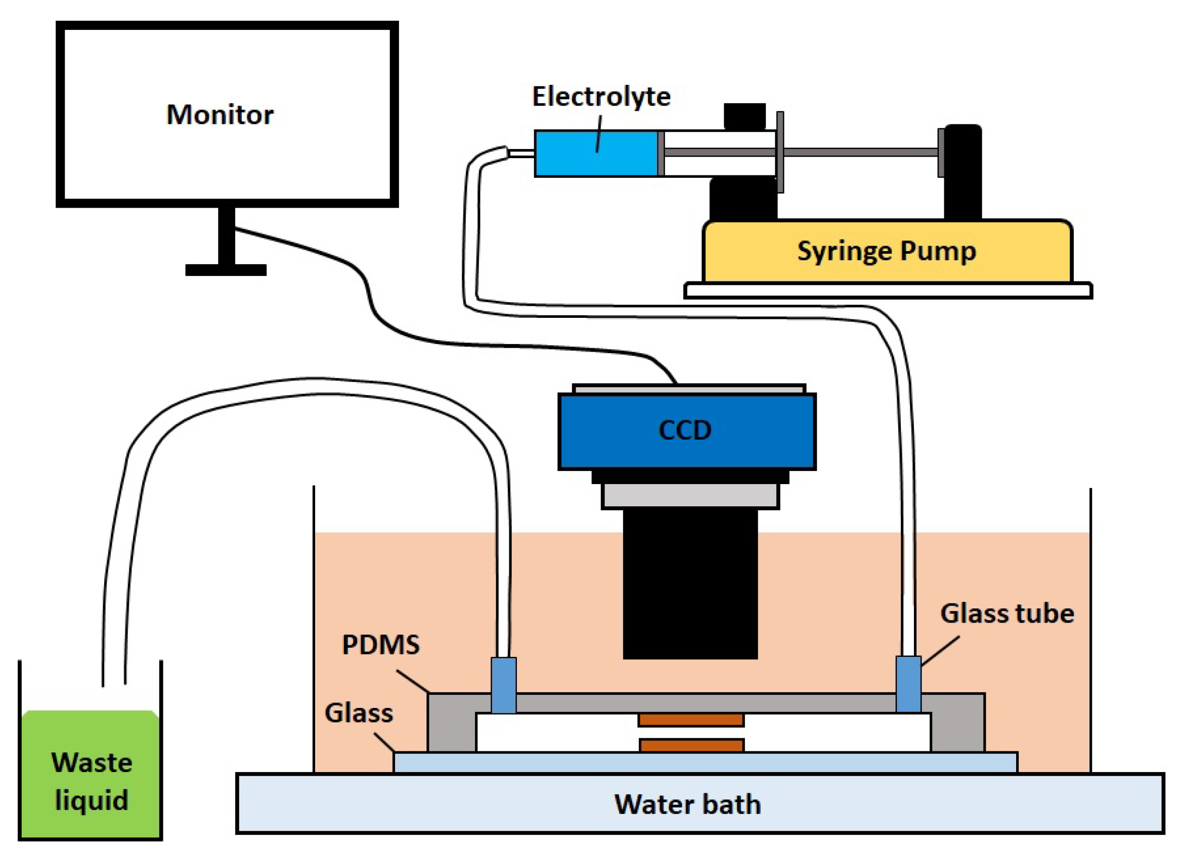
An electrolyte with copper ions and formaldehyde flows in micro-channel between two parallel glass sheets (
Figure 1). One piece of the sheet is partially glued on a copper plate whose longer side coincides with an edge of the inlet. Electroless copper plating was conducted in a water tank controlled at 50 °C with in situ recording via stereomicroscope (charged coupled device 311 digital camera CCD).
Results show that the bubbles are not only appearing on the copper plate, but also near the top glass sheet. In the video, one can see that there were several bubbles going to the top from the center or the bottom side of the channel. The bubble size distribution was not measured and it ought to be done in the future and combined with numerical simulations as in [
37]. The measurement of the bubble densities in the experiment is possible by means of acoustic, optical, and laser diffraction approaches [
38]. However, these techniques are hard (or expensive) to be adapted on a microfluidic scale.
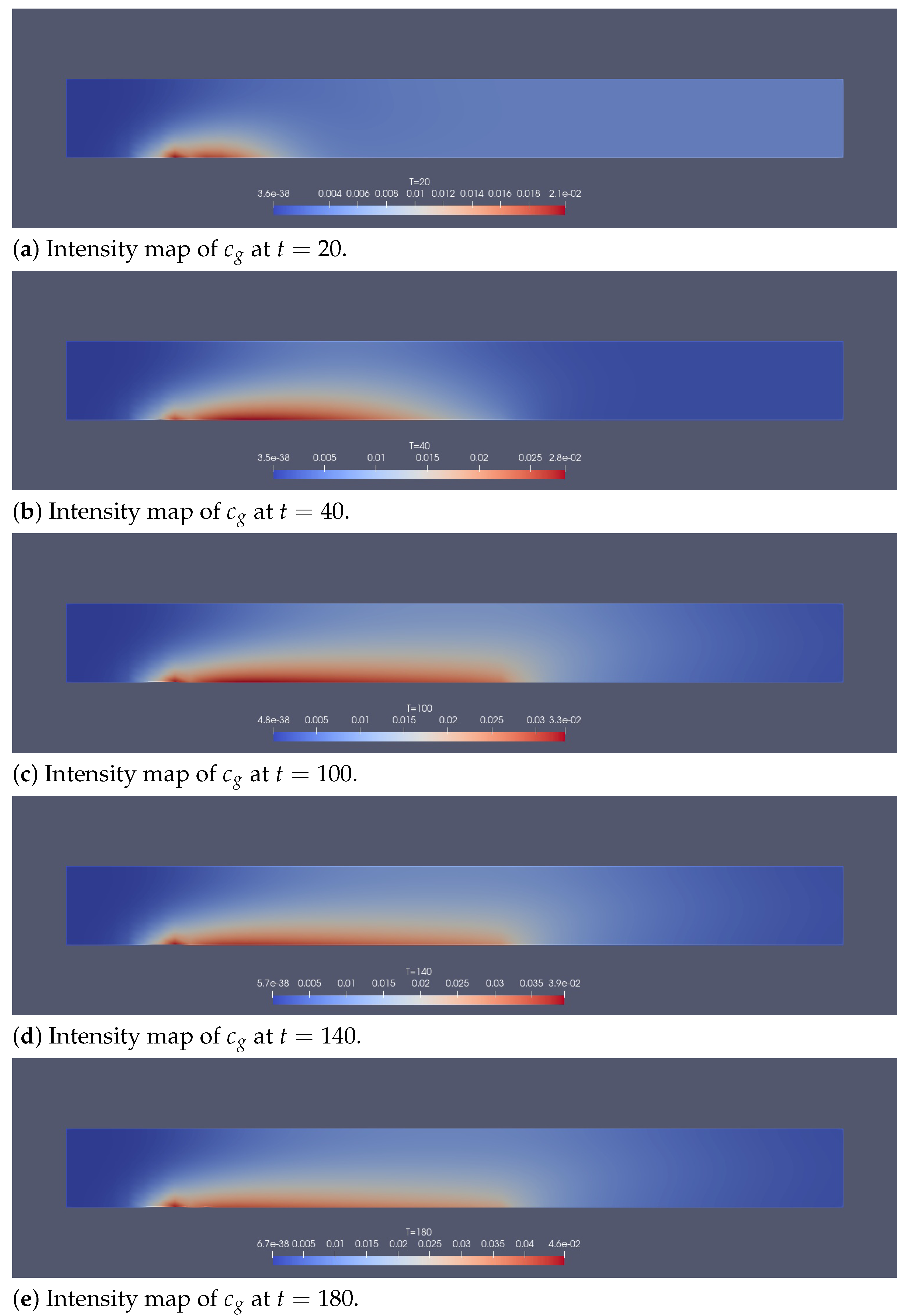
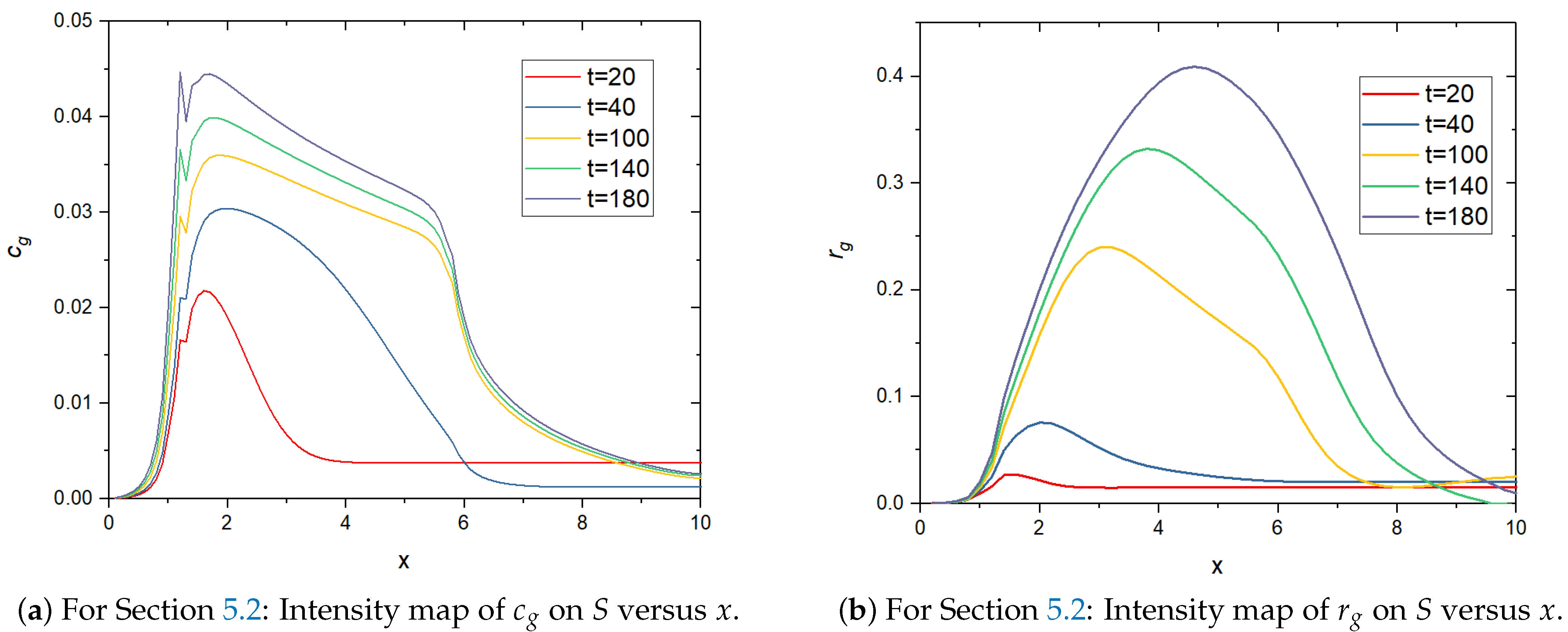
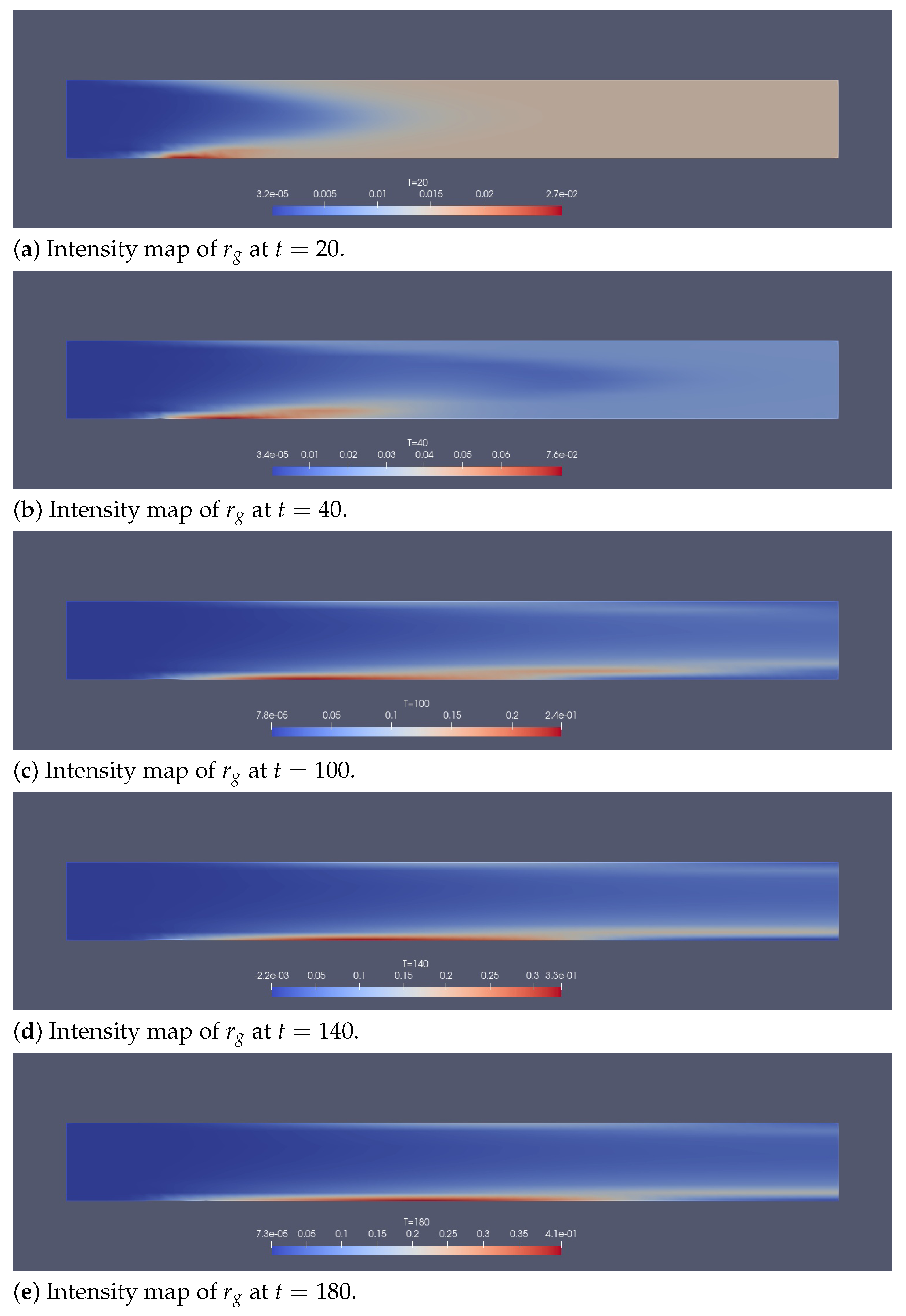
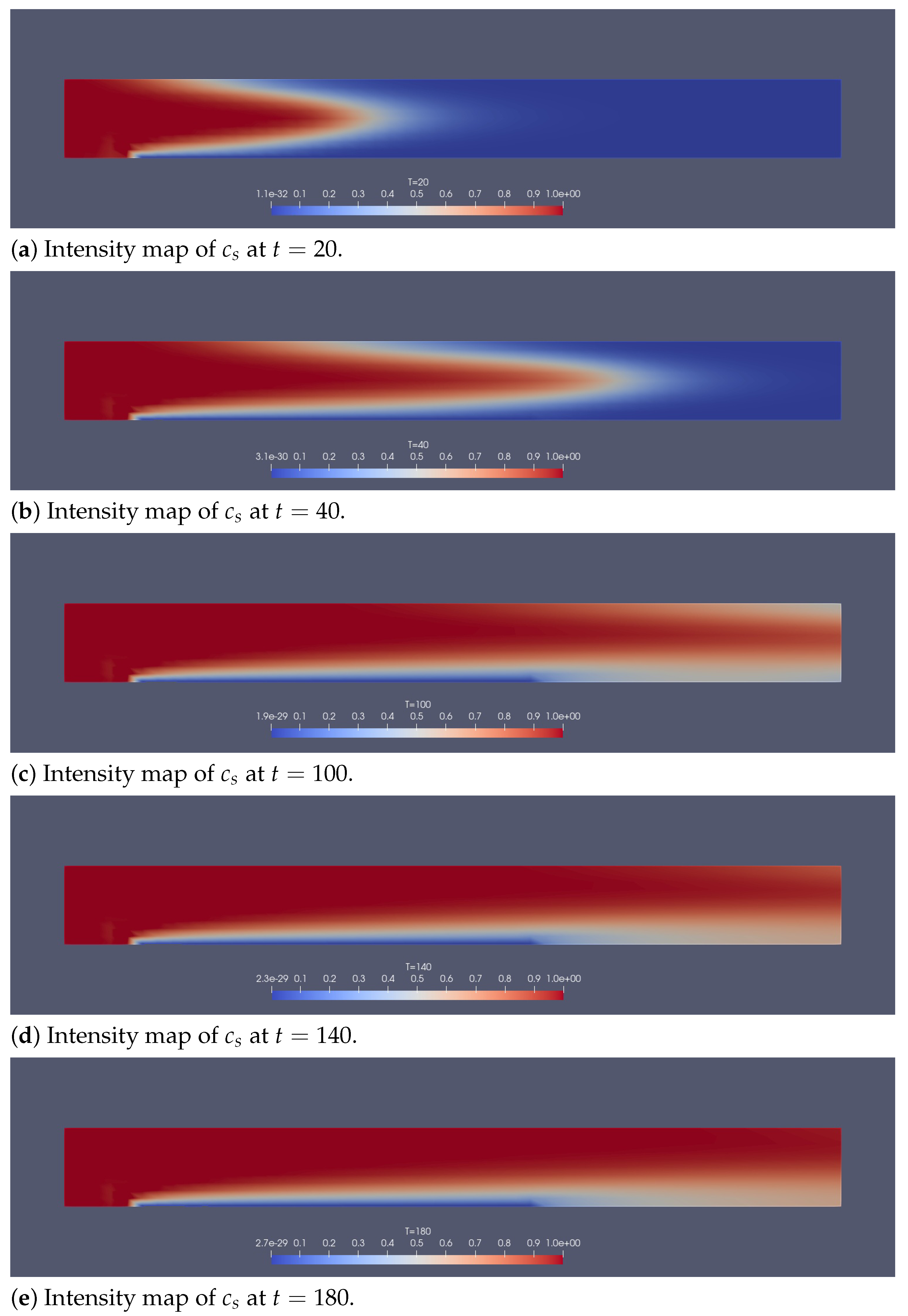
The computer simulations qualitatively arrive at the same conclusion. The experiment indicates that the clustering of bubbles happens on both the top side and the bottom side of the channel. Second, the numerical simulation predicts that most bubbles are generated at an early stage and near the inlet. The experiment shows that the bubble generation is more exuberant near the inlet. This observation coincides with that of
Figure 2 and
Figure 3a. The region near the inlet at
is of the highest concentration of dissolving hydrogen gas. In addition, large bubbles were observed at the back end of the copper plates, which is also the case numerically as seen in
Figure 3b.
The comparison is qualitative but sufficient to assert that the simulation software is a more powerful tool to prototype future industrial designs. Potentially, it seems more reliable than experiments and it gives detailed information on the free boundary and on the speeds and concentrations of the chemical, which is highly important for the design of commercial systems. Thus, we are confident in the future of the numerical method. The mathematical properties of robustness, stability, and convergence, verified here numerically, are a certification of the computer software for future use.
2. Modeling Equations for Liquid-Gas Flow
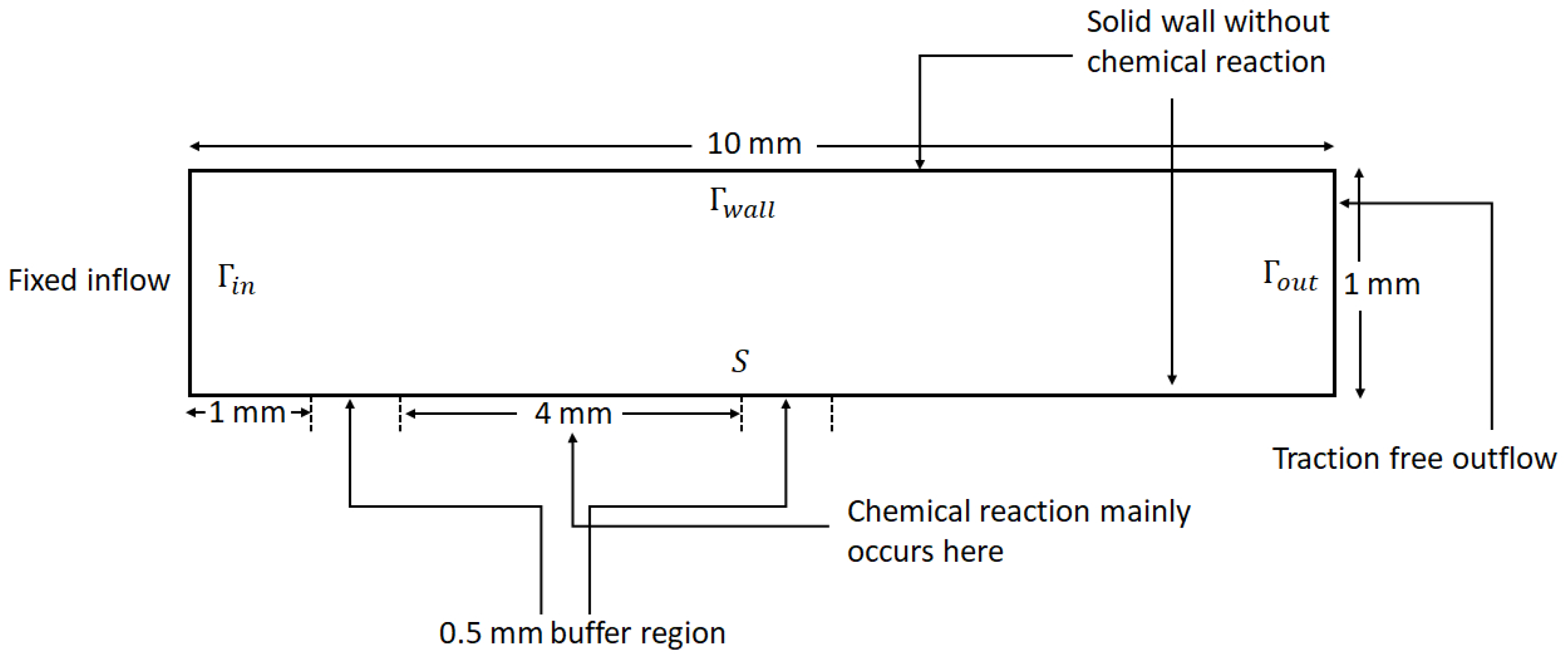
Let
be the time-dependent physical domain which is a thin channel between a top and a bottom plate. The boundary of
consists of the inlet
, the outlet
, the solid wall
, and the reacting surface
(see
Figure 4).
2.1. Volume Averaging
We review the derivation proposed by Ni and Beckermann [
39].
Let be an small open set to be observed in and the set occupied by phase k and bounded by the interface . Assume that and . Let be a outer normal to and the normal velocity of .
Let
be a function of a slow variable
x and a fast variable
y due to the phase change. The volume average of
in phase
k is
where
is the indicator function of the domain of phase
k and
, assumed constant. The intrinsic volume average is defined as
The volume fraction
has the properties
and
Some useful averaging formulas are listed below [
40,
41]:
In principle, one should also introduce fast and slow time variables but it is assumed that spatially averaged functions are no longer varying fast in time.
2.2. Mass Conservation
We consider a gas and a liquid phase. Let
be the density of gas,
the density of liquid. We have the mass conservation for both phases (
l for liquid and
g for gas):
where
is the mass gained owing to the precipitation of dissolved gas,
is the mass loss when liquid evaporates into gas;
,
are the volume averaged fluid flow of gas and liquid, respectively. Since the mass gained in gas balances the mass lost in liquid, we have
For chemical species, we assume that the ions are transported only by the liquid electrolyte. Let
be the volume averaged concentration of metallic ions destined to be deposited on the reacting surface,
the volume averaged concentration of dissolved gas, and
,
the volume averaged concentration of other chemical species participating to the chemical reactions. The equations for the concentrations are
where
,
are interfacial terms due to the phase change. By (
3), we can rewrite the above equation as
where
are the diffusion coefficients. In particular, since the gas is consumed by the phase change, by assuming that the gas precipitation is linearly dependent on the dissolving gas concentration [
42,
43], we have
In the above,
is the interface velocity of
and
K is a constant independent of
,
;
is the saturated concentration of the gas,
is the reciprocal of the molar mass of the gas,
Moreover,
,
can be estimated by (see
Appendix A)
For incompressible fluids, a volume conservation is derived from (
3):
By (
4), the above reduces to
Recall that the physical domain is occupied either by gas or liquid, therefore at all times.
2.3. Equations of Motion
Let
,
be the viscosities of gas and liquid. The volume averaged Navier–Stokes equations are used for momentum balance (see [
39]):
where
are pressure, drag and external force terms. Following [
24,
39]
where
is a drag coefficient, and the external force are in fact the interfacial terms
and
is twice the symmetric gradient of
;
and
can be estimated by (see
Appendix A)
In view of (
11), following [
44,
45], we assume a constitutive relation
in order to close the system of equations. The velocity fields of both phases are assumed to be 0 outside their own single phase region, respectively. Consequently, and by (
3) and (
12), the momentum equations simplify to
2.4. Boundary Conditions
We consider a fluid flow from an input boundary
to an output boundary
with a solid wall at the bottom,
:
The boundary conditions for
,
are
where
is a fixed positive small constant.
The boundary conditions for the concentrations of chemicals are, with
given:
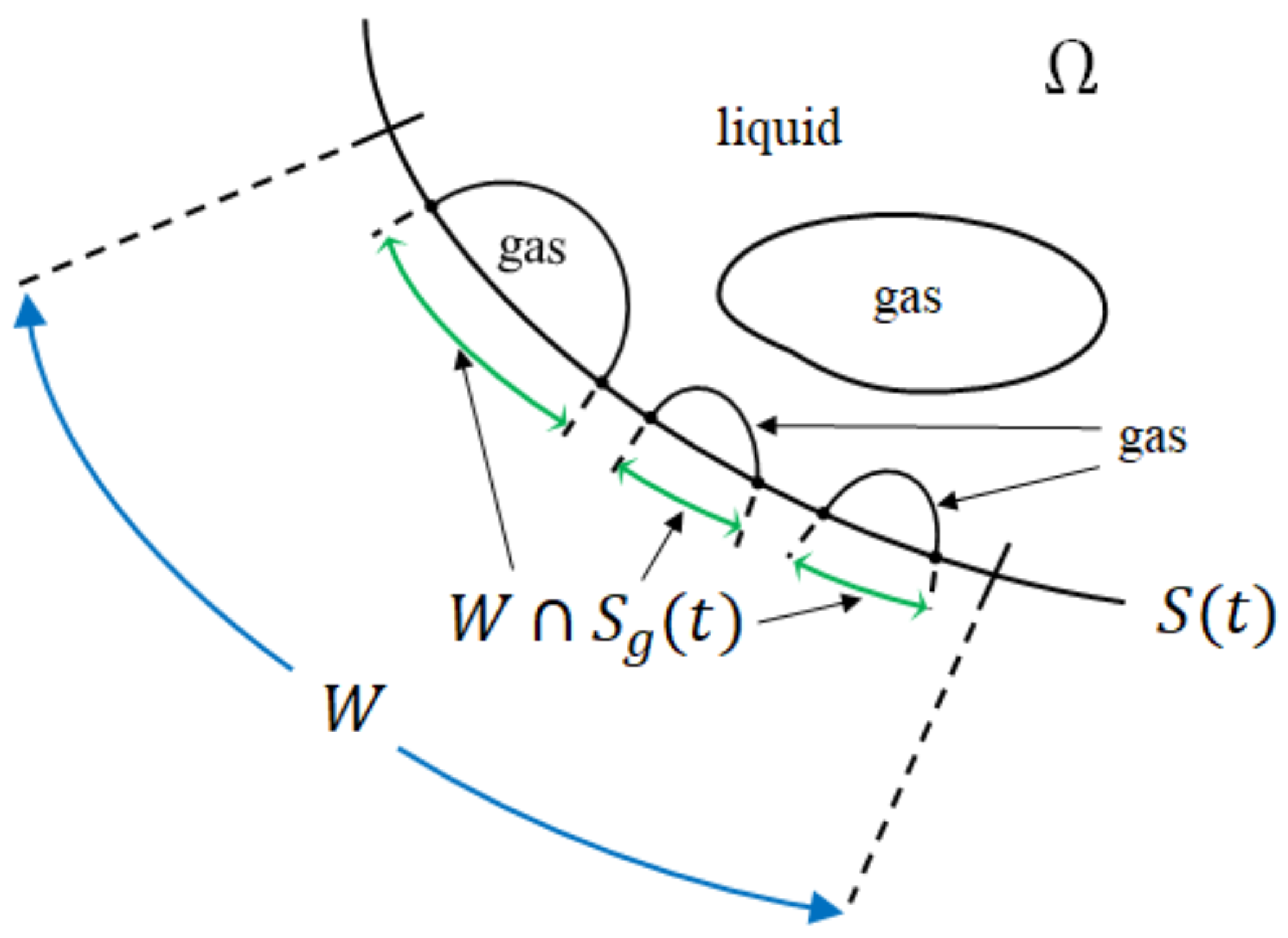
Referring to
Figure 5, if
is the reaction surface, we denote
the region occupied by the liquid and
the region occupied by gas. Choosing an arbitrary subset
, the surface reaction takes place only on
. Assuming that the concentration profile is uniform near the small region
W, we have:
. Therefore by dividing both sides by
:
for a positive number
indicating the chemical equivalence for gaseous molecular generation;
F is the Faraday constant, and
z is the atomic number of the material.
is the current density satisfying the Butler–Volmer equation
where
R is the gas constant,
are the chemical potentials of species
j,
is the temperature,
,
,
are constants, and
is given by writing electrical neutrality:
On
, the fluid velocity induced by the deposition is
where
is a constant.
Finally,
moves according to
2.5. Single-Phase Flow
If there is no gaseous phase in the system and no dissolved gas in liquid, i.e.,
, then
and
and mass conservation reduces to
. The convection–diffusion of chemicals become,
and the fluid system reduce to the Navier–Stokes equations:
4. Finite Element Implementation
For simplicity, the physical domain is assumed to be a two-dimensional polygonal domain.
4.1. Mesh
Let
be an affine, shape regular (in the sense of Ciarlet [
48]) family of mesh conforming to
. The conforming Lagrange finite element space of degree
p on
is
where
is the space of polynomials of degree
p of
.
Let be the nodal Lagrange basis of . If the vertices are denoted by , then . Let be the support of and let . If E is a union of triangles, define . Finally, the local minimum mesh size of is and the global minimum mesh size is .
We assume that the connectivity of the mesh never changes with time.
4.2. Spatial Discretization
We use the Hood–Taylor element: the velocities are in and the pressure is in . For the volume fractions and the concentrations we use also .
Recall that the nodes of are the vertices and the middle of the edges. Denote by the nodal Lagrange basis of . As before , and .
On the boundaries where Dirichlet conditions are set, the functions are known. We denote and , the corresponding spaces where basis functions attached to a Dirichlet node are removed.
4.2.1. Mass Fractions
Given
and
, find
satisfying the Dirichlet boundary conditions and such that
where
for
,
. Then we let
.
Remark 2. A modification similar to (
39) will insure the positivity of
.
4.2.2. Concentration Profiles
Given
,
,
, find
such that
subject to
where
is the last component of
and
for
defined by (
20).
4.2.3. Two-Phase Flow
Given
,
,
, and
, find
,
and
such that
for all
,
and
.
4.3. Fixed Point Iterative Solution of (50) and (51)
The system (
50) and (
51) is nonlinear. Algorithm 1 is proposed.
| Algorithm 1: A semi-lineariazation for solving (50) and (51). |
Let be defined by (42).
Data: Set .
for do
|
![Fluids 06 00371 i001]() | Set ,
Find and p sastifying the Dirichlet conditions and such that, and
|
end
Set .
|
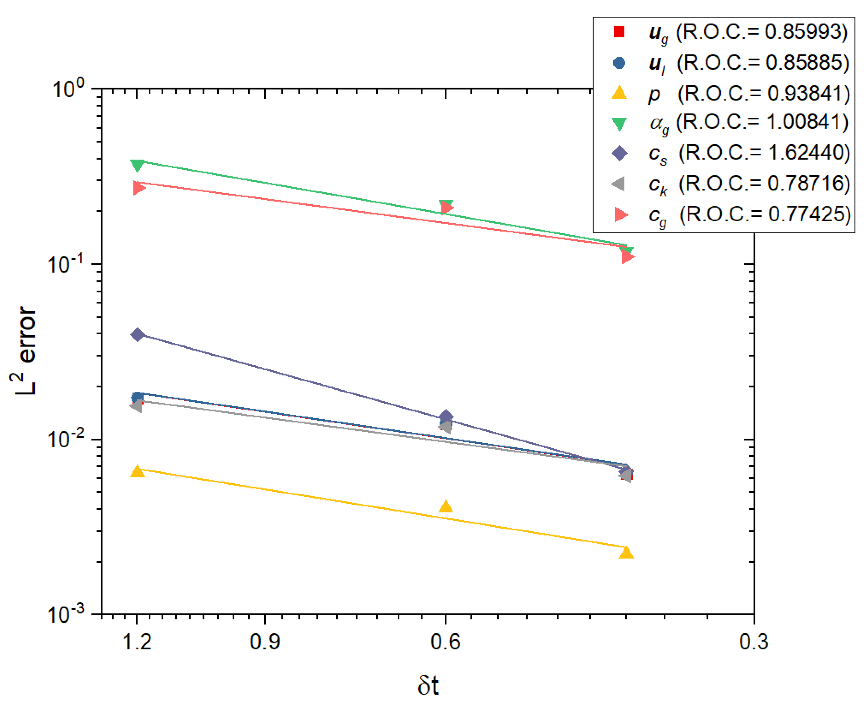
4.4. Consistence and Stability
Variational formulations discretized by finite element methods inherit the stability and consistency of the continuous equations. The LBB theorem applies also to the Hood–Taylor element for velocity pressure problems. Therefore, as in the continuous case, the norms of are less than times the norms of . If we could show that is bounded, then it would imply that the scheme converges when .
4.5. Solvability of the Linear System in Matrix Form
Let , , for some constant , .
To study the solvability of (
50)–(
51), we consider a simpler case with
on
, and take the linearized approximation on the drag force terms. The problem reads: Find
and
satisfying
where, for
,
,
On the basis of
and
, we can write
More precisely is for and .
Problem (
53) can be formally expressed as a system of linear equations:
where
is a
matrix,
and
are
vectors. Note that
has the form
with, for
Proposition 1. The linear system (56) is uniquely solvable. Proof. According to the LBB theorem [
46] the saddle point problem (
52) is well posed when for
, there exists
such that
Therefore has full rank and is non singular. □
4.6. Iterative Process
At each time step, (
47), is solved first, then (
48) and (
49) is solved iteratively by using a semi-linearization of the nonlinear boundary terms. Then (
50) and (
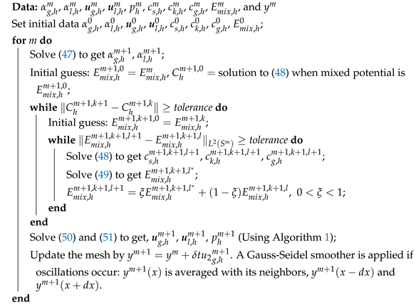
51) is solved iteratively by a semi-linearization of the nonlinear terms; each block involves the solution of a well posed symmetric linear system. Finally
is updated by (
23). Algorithm 2 summarizes the procedure.
Note that the computational domain is .
6. Comparison with Experimental Results
To validate the numerical method on a real-life problem, an experiment for reproducing the numerical study in
Section 5.2 is conducted. Here, we shall show that the experimental result can be qualitatively fitted by the numerical simulation.
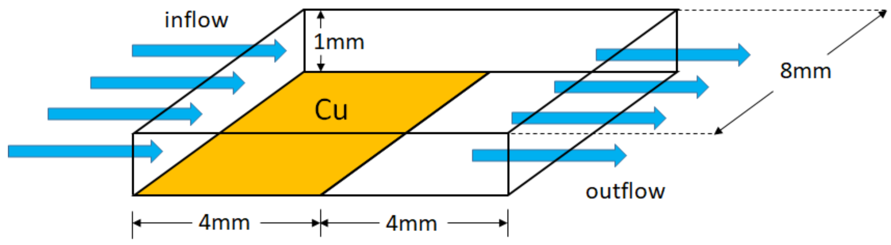
The experimental setting is described as the following: A micro-channel is enclosed by two sheet glasses of size 8 mm × 8 mm and another two of size 8 mm × 1 mm, which form a rectangular channel. The electrolyte goes in the channel from the left and exit on the right. One piece of the square sheet glasses is partially glued on a copper plate of size 8 mm × 4 mm, where the longer side of the copper plate coincides with an edge of the inlet (see
Figure 1 for geometry setting). The inflow is set to be of average velocity 0.115 mm/s. At inlet, the copper ion concentration is
mol/m
3 and the formaldehyde concentration is
mol/m
3. Here, the inlet concentrations
and
are the reference concentrations for copper ion and formaldehyde, respectively. We further define the reference concentration of the hydrogen gas to be
mol/m
3. Other physical parameters are given in
Table 3. Some parameters, for example, reference current densities
, and
, may not be exactly same as what are given in
Table 3. Nevertheless, they are acceptably closed to reality, or at least in the same order.
6.1. Experimental
To fabricate the test vehicle, a 4 inch glass wafer was first sputtered with 30 nm chromium and 200 nm copper which served as an adhesion layer and seed layer, respectively. The wafer was then diced into each 8 mm × 8 mm glass dies. To ensure a significant comparison between the regions being plated or not, each test die was half immersed in SPS (
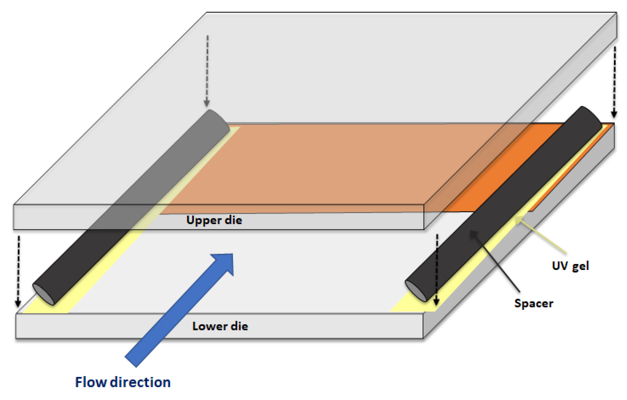
) solution and hydrochloric acid to remove the copper and chromium layer. The glass die turned out half transparent and half coated with copper where the electroless copper plating took place. Thereafter, a fully transparent glass, which was identical to the size of the test die, was face-to-face aligned and bonded via using a flip-chip die-bonder in order to obtain a clear observation view. Two tungsten wires which were 8 mm in length and 2 mm in diameter were glued by UV gel and placed on the periphery of the test die for the purpose of restricting the flow direction and defining the height between the dies (see
Figure 18).
The test vehicle was then subjected to a micro-fluidic system composed of a PDMS mode containing a micro-fluidic channel and a bottom glass. Clips were used to seal the micro-fluidic system and prevent the leakage of electrolyte. A peristatic pump was used to control the flow and connect the micro-fluidic system with a silicone tube. Prior to the electroless plating, the test vehicle was immersed in
sulfuric acid to remove copper oxide. Finally, the electroless copper plating was conducted in a water tank controlled at 50 °C with in situ recording via stereomicroscope (charged coupled device digital camera CCD). The electrolyte PHE-1 Uyemura possessing the given reference concentrations
of (complexed) copper ion and
of formaldehyde was used for the experiment. The complete equipment setup is described in
Figure 19.
6.2. Results
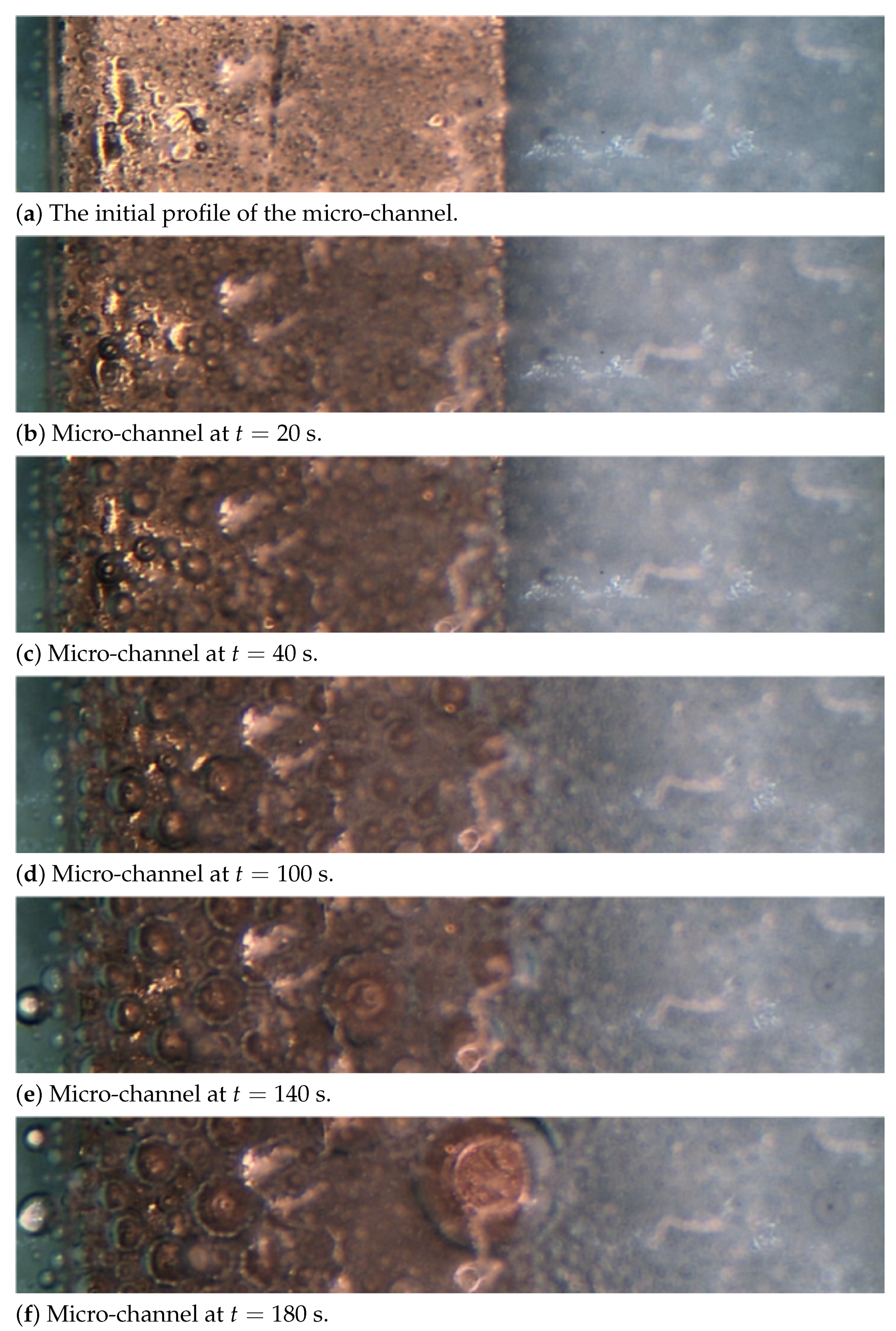
Experimental results (see
Figure 20) show that the bubbles are not only appearing on the copper plate, but also appearing on the top. In the video, one can see that there were several bubbles going to the top from the center or the bottom side of the channel. The region above the glass becomes darker with time. The simulation results (see
Figure 13) qualitatively arrive at the same conclusion. The experiment indicates that the clustering of bubbles happens on both the top side and the bottom side of the channel. Second, the numerical simulation predicts that most bubbles are generated at an early stage and near the inlet. The experiment shows that the bubble generation is more exuberant near the inlet in comparison with other regions at
. This observation coincides with that of
Figure 2 and
Figure 3a. The region near the inlet at
is of the highest concentration of dissolving hydrogen gas. In addition, large bubbles were observed at the back end of the copper plates (i.e., region near (x,y) = (6,0) corresponding to
Figure 4), which is also the case in
Figure 3b.
6.3. Discussion
For an electroless plating process accompanying gas generation, the bubble distribution with respect to time, in the micro-channel, is the most important index for evaluating the quality of deposition. To measure it quantitatively, a high-quality optical system installed in the micro-channel is indispensable. For example, several types of fiber optical probes have been used to measure the particle (or bubble) size and distribution in a channel flow (or micro-channel flow) [
53,
54,
55,
56]. However, such an optical system is difficult to install in our case because there is no appropriate place to set up the light source and the detector in the micro-channel. The signal interference caused by the copper plate or glued gel on two sides is almost inevitable.


