Abstract
A detailed study of solar wind turbulence throughout the heliosphere in both the upwind and downwind directions is presented. We use an incompressible magnetohydrodynamic (MHD) turbulence model that includes the effects of electrons, the separation of turbulence energy into proton and electron heating, the electron heat flux, and Coulomb collisions between protons and electrons. We derive expressions for the turbulence cascade rate corresponding to the energy in forward and backward propagating modes, the fluctuating kinetic and magnetic energy, the normalized cross-helicity, and the normalized residual energy, and calculate the turbulence cascade rate from 0.17 to 75 au in the upwind and downwind directions. Finally, we use the turbulence transport models to derive cosmic ray (CR) parallel and perpendicular mean free paths (mfps) in the upwind and downwind heliocentric directions. We find that turbulence in the upwind and downwind directions is different, in part because of the asymmetric distribution of new born pickup ions in the two directions, which results in the CR mfps being different in the two directions. This is important for models that describe the modulation of cosmic rays by the solar wind.
1. Introduction
Turbulence in solar wind plays an important role in many aspects of plasma behavior: (i) the observed nonadiabatic radial profile of the solar wind temperature [1,2,3,4,5,6,7,8,9,10,11,12,13,14,15,16,17,18,19,20,21,22,23]; (ii) the scattering of the solar energetic particles [24,25]; (iii) the heating of the coronal plasma to millions of degrees Kelvin and the acceleration of the solar wind from a subsonic to a supersonic speed [26,27,28,29,30,31,32,33,34,35,36,37,38,39,40], (iv) the transport of cosmic rays throughout the heliosphere [22,41,42,43,44,45], and (v) the increase in the solar wind proton and electron entropy [20,46,47].
Since the early space age observations of solar wind turbulence [48,49,50,51,52,53,54,55,56,57], interplanetary fluctuations have been described either as evidence of a turbulent solar wind [48] or as the superposition of forward propagating Alfvén waves [50]. These early results are contradictory. The turbulent characteristics of the solar wind are based on the idea that the solar wind plasma and magnetic field fluctuations exhibit a power-law like spectra as predicted by a Kolmogorov [58] or Kraichnan [59] phenomenology. However, the strongly Alfvénic character of the solar wind fluctuations observed by Belcher and Davis [50] suggests the existence of pure Alfvén waves, and does not, therefore, support nonlinear interactions between counter-propagating Alfvén waves. In the latter case, the observed unidirectional propagation of Alfvén waves that exhibit a Kolmogorov-like power law [60,61] has been ascribed to the interaction with dominant quasi-2D turbulence [62]. Coleman [48] suggested that sheared solar wind flows that are generated by the difference in fast and slow solar wind speeds, generates low-frequency MHD turbulence in the inner heliosphere. Tu et al. [63] proposed a model to explain the radial evolution of the power spectrum of the Alfvénic fluctuations observed by 1 and 2 in the inner heliosphere between 0.3 and 1 au [51]. In their model, they assumed that most of the fluctuations correspond to forward propagating incompressible (Alfvénic) wave modes, with fewer of the fluctuations corresponding to backward propagating wave modes. This indicates that there is a weak interaction between counter-propagating modes, which is consistent with Coleman [48] in the sense that the turbulent shear source generates backward propagating wave modes [17,64].
The modeling of the transport of incompressible interplanetary fluctuations began with the Wentzel–Kramers–Brillouin (WKB) theory. WKB theory describes the transport of linear, non-interacting MHD Alfvén waves in an inhomogeneous background [65,66,67,68,69]. The description incorporates convection, wave propagation, and expansion effects, but does not consider the nonlinear interaction between forward and backward propagating Alfvén waves. Forward and backward propagating Alfvén waves interact on the nonlinear timescales , where are correlation lengths corresponding to the Elsässer energies . Similarly, the propagation of Alfvén waves introduces the Alfvénic timescales , where are the correlation lengths along the direction of the magnetic field, and is the magnitude of the Alfvén velocity. If , the counter-propagating modes experience many interactions before their energy is transferred into smaller scales [59,70]. This is known as a weak turbulence. If , the Alfvénic fluctuations undergo multiple decays before they interact. This is known as a strong turbulence. When the two timescales are comparable, i.e., , this leads to the scaling of , and is known as a “critical balanced” state [71].
The outline of the paper is as follows. In Section 1, we present an overview of incompressible MHD turbulence transport models, and in Section 2, we discuss 3D solar wind turbulence models. In Section 3, we discuss 1D steady-state turbulence models, including the incorporation of electrons, and present comparisons between the theoretical results with those measured by , 2, 2, () in the upwind direction, and with 10 in the downwind direction. In Section 4, we derive the turbulence cascade rate for the energy in forward and backward propagating modes, the total turbulent energy, the cross-helicity, the residual energy, the turbulent kinetic energy, and the turbulent magnetic energy, and discuss the results. Section 5 discusses the cosmic rays diffusion tensor and its relation to the turbulence transport models. Finally, further discussion and conclusions are found in Section 6.
2. Incompressible MHD Turbulence Models
The fluctuating Elsässer variables [72] (where is the fluctuating solar wind speed, the fluctuating the magnetic field, the proton mass density, and the magnetic permeability) define the forward and backward propagating modes [63,73,74,75,76,77,78]. The incompressible MHD transport equations can be expressed in terms of the Elsässer variables as [73,74,75],
where I is the identity matrix, the nonlinear terms, the solar wind speed, the Alfvén velocity, and are sources of turbulence. When constructing ensemble-averaged moments of the Elsässer variables using (1), such as or etc., terms inside the squared brackets are introduced like , which is an MHD analog of the hydrodynamic Reynolds stress. Due to the presence of the terms, the backward and forward propagating modes interact through the small-scale fluctuations, and large-scale solar wind speed and magnetic field.
The advantage of the transport Equation (1) is that it includes the nonlinear interaction between and , and introduces the cross-helicity and the residual energy (definitions given below), which are measures of the Alfvénicity of the solar wind turbulence. The turbulence transport model equations are, therefore, useful to study the radial evolution of MHD turbulence, Alfvénicity, and applications, such as coronal heating, and the solar wind heating throughout the heliosphere.
Starting from Equation (1), Zank et al. [76] developed a simple model comprising two coupled turbulence transport equations for the turbulent magnetic energy density (=, where is the fluctuating magnetic energy) and the correlation length of the magnetic field fluctuations . The Zank et al. [76] model was compared successfully with turbulent magnetic energy observations measured by 1, 2 and 11 between 1 and 40 au.
Matthaeus et al. [4], Smith et al. [5], and Smith et al. [6] included the dissipation of magnetic energy [76] in the proton temperature equation to study proton heating throughout the heliosphere [3,8,9]. Matthaeus et al. [4], Smith et al. [5], and Smith et al. [6] found that the radial profile of the solar wind temperature is similar to that observed by 11 and 2, including the observed temperature increase in the distant heliosphere. Of particular note was an observed temperature increase [1] in the solar wind temperature beyond ∼25–30 au. This was explained by Williams et al. [3] as being due to the dissipation of PUI-driven waves in the outer heliosphere. Adhikari et al. [16] extended the Zank et al. [76] model by using time-dependent boundary conditions and time-dependent turbulent sources. They compared their model results with 2 measurements, and found periodic changes in the magnetic energy density, correlation length, and the solar wind temperature, especially beyond au.
In developing an incompressible MHD turbulence model, Matthaeus et al. [79] proposed that the radial evolution of the normalized cross-helicity vary [80], but also assumed that the normalized residual energy (the energy difference between the fluctuations in the velocity and magnetic field) is constant. Later, Breech et al. [10] extended the turbulence transport model to study the evolution of turbulence energy, normalized cross-helicity, and the turbulent correlation length from the inner to outer heliosphere by assuming that the normalized residual energy is constant, and the solar wind is super-Alfvénic, i.e., . Therefore, the Breech et al. [10] model cannot be used for sub-Alfvénic flows, i.e., , where the Alfvén velocity is larger than the solar wind speed.
The incompressible MHD turbulence model was further developed by Zank et al. [77] to include the residual energy, various correlation lengths, and the Alfvén velocity, making it suitable for sub-Alfvénic flows. Zank et al [77] used Equation (1) to develop a six coupled equations turbulence model that describes the transport of the total energy density, cross-helicity, residual energy, and correlation lengths corresponding to forward and backward propagating modes and the residual energy. To model the dissipative terms for the various transport equations, Zank et al. [77] used a single-point closure related to that of von Kármán and Howarth [81], and further developed [10,76,82,83,84]. The six coupled turbulence transport equations of Zank et al. [77] describe the transport of turbulence in inhomogeneous sub-Alfvénic and super-Alfvénic flows. The Zank et al. [77] turbulence equations are quasi-linear in the spatial evolution operators, and nonlinear in the dissipation terms.
Adhikari et al. [17] studied the evolution of turbulence in the super-Alfvénic solar wind flow from 0.3 to 75 au using the Zank et al. [77] turbulence model and 2 measurements. They compared their model results with 2, , and 2 measurements, and found that (i) shear driving is responsible for the in situ generation of backward propagating modes; (ii) the correlation lengths corresponding to forward and backward propagating modes increase with distance, and are approximately equal beyond ∼30 au, and (iii) the fluctuating kinetic and magnetic energies are approximately equal beyond ∼30 au.
Adhikari et al. [20] developed a conservative formulation of the coupled solar wind and incompressible MHD turbulence transport model equations using the Zank et al. [77] turbulence model. They showed that not only the pickup ions, but also stream-shear leads to a decrease in the solar wind speed. They showed that the sum of the solar wind flow (kinetic plus enthalpy) energy and turbulent (magnetic) energy is constant, illustrating that kinetic solar wind energy is transferred into turbulent energy via stream-shear and pickup ion isotropization, which then in turn heats the solar wind via the dissipation of turbulence.
Consider the following moments of the Elsässer variables,
where is twice the total energy of the fluctuations per unit mass (or the sum of the square of the fluctuating plasma and Alfvénic velocity), is the cross-helicity of the fluctuations (or a measure of the obliquity of the fluctuating velocity and magnetic field vectors), and is twice the difference between the fluctuating kinetic and magnetic energy per unit mass. The variable is the energy in forward/backward propagating modes. Similarly, the following relations hold [77,85],
where is the Alfvén ratio, the normalized cross-helicity, the correlation length corresponding to forward/backward propagating modes, the correlation length corresponding to the residual energy, and the correlation lengths corresponding to the velocity/magnetic field fluctuations.
Similarly, we can also introduce the following relations,
where, and denote the correlation functions corresponding to forward/backward propagating modes, and the residual energy. The prime denotes the spatial lagged Elsässer variables separated by the distance y.
The detailed derivation of the six coupled turbulence transport equations is presented in Zank et al. [77], and the equations are given by,
where a and b are the structural similarity parameters related to the large-scale velocity , and the Alfvén velocity , respectively. The parameters a and b can be chosen freely, and choosing and or and produces 2D or 3D mixed tensors [83]. In Equations (5)–(7), the first three terms on the lhs are similar to the standard WKB model, while the remaining terms describe the indirect mixing and coupling of forward and backward propagating modes. The first two terms on the rhs are the nonlinear terms, and the latter two terms indicate turbulence sources. The nonlinear dissipative term for the total turbulent energy is derived by following a Kolmogorov phenomenology, and has been verified by numerical simulations [86]. The nonlinear terms can also be expressed using instead an Iroshnikov–Kriachnan phenomenology e.g., [13].
3. 3D Solar Wind–Incompressible MHD Turbulence Model
A global turbulence model has been developed by coupling various forms of the 3D turbulence transport model with a global MHD model of the solar wind [14,21,22,45,87,88,89,90,91,92,93]. Usmanov et al. [14] developed a self-consistent 3D solar wind-turbulence model to study the effect of turbulence on large-scale solar wind properties and solar wind heating from 0.3 to 100 au. Usmanov et al. [87] extended their three-dimensional solar wind model to incorporate turbulence transport and pickup ions as a separate fluid. The global MHD model is based on solving the large-scale Reynolds-averaged MHD equations when coupled to pickup ions and the associated generation of turbulence from 0.3 to 100 au. They confirmed well-known effects of pickup ions on the large-scale solar wind, such as the slowing down of the solar wind speed due to the momentum loss from the solar wind protons to pickup ions, and the compressed azimuthal magnetic field in the outer heliopshere [94]. They also found that the decelerated solar wind speed and the pickup ions weaken corotating interaction regions (CIRs), confirming results by Zank et al. [95] and Rice and Zank [96]. Usmanov et al. [88] further extended the 3D MHD solar wind and turbulence model to include eddy viscosity, turbulent resistivity, and turbulent heating. Usmanov et al. [88] considered a system of co-moving solar wind protons, electrons and interstellar pickup ions, each species having a separate energy equation. They presented three-dimensional distributions of the mean-flow and turbulence parameters throughout the heliosphere under the given boundary conditions at the coronal base, finding that the effect of the eddy viscosity, and velocity shear on the mean-flow parameters increases the solar wind proton and electron temperatures. Usmanov et al. [89] further extended their 3D solar wind turbulence model to include electron heat conduction, radiative cooling, Coulomb collisions, Reynolds stresses, eddy viscosity, and turbulent heating of protons and electrons. Chhiber et al. [45] used the 3D solar wind-turbulence model of Usmanov et al. [14] to study the cosmic ray diffusion tensor throughout the heliosphere [41].
In a related study, Kryukov et al. [90] developed a 3D solar wind turbulence model that incorporates pickup ions and solar wind heating over a heliocentric distance 1–80 au. Like the 3D MHD models of Usmanov et al. [14,87,88,89], Kryukov et al. [90], and Chhiber et al. [93] incorporate the back reaction of turbulence on the global MHD flow by including both the turbulent heating term and Reynolds-averaged turbulence terms in the MHD model. However, these papers combined the simpler turbulence model [10,76] with 3D MHD solar wind models. Similarly, they assumed a constant normalized residual energy in the turbulence model.
Wiengarten et al. [21] developed a 3D model in which they coupled turbulence transport equations with the Reynolds-averaged ideal MHD equations, and applied their model to study the propagation of coronal mass ejections (CMEs). Wiengarten et al. [21] introduced the effect of turbulence driven by shear, which was not taken into account in Usmanov et al. [14]. They found that a CME enhances turbulence levels and reduces the cross-helicity, but the overall effect of CMEs is negligible. Wiengarten et al. [22] coupled a two-component turbulence model of Oughton et al. [15] self-consistently with the large-scale MHD equations, and calculated the mean-free path and the drift lengthscale of cosmic rays throughout the heliosphere.
Finally, Shiota et al. [91] coupled a more sophisticated turbulence model, Equations (5)–(9) of Zank et al. [77], with a large-scale 3D MHD solar wind model [97] to study the basic physical changes of turbulent transport in a more complex structured solar wind. The model included the inhomegeneity of the background solar wind and IMF, and sources of turbulence. To obtain a simple structure for the solar wind, Shiota et al. [91] assumed two steady magnetic field configurations, such as an outward monopole magnetic field whose intensity is spherically symmetric at R, and a tilted dipole magnetic field at an angle 30 from the rotational axis of the Sun. Shiota et al [91] also considered (i) a spherically symmetric constant solar wind speed of 400 kms or 600 kms, and (ii) a bimodal (fast and slow) solar wind flow. In the latter case, the speed is determined by the titled dipole potential field and the Wang–Sheely–Arge 2000 [98,99] model for coronal magnetic fields. Shiota et al [91] found that the non-axisymmetric solar wind speed distribution with a spherically symmetric IMF enhances the energy in backward propagating modes and the normalized residual energy in the interaction region.
4. Incompressible MHD Turbulence Model: Proton and Electron Heating
Most of the turbulence transport models include proton heating [1,2,3,4,5,6,7,8,9,10,11,12,13,14,15,16,17,18,19,20,21,22,23], and neglect electron heating. Electrons carry about half of the thermal energy of the plasma, which indicates that the role of electrons should not be neglected. Electron effects includes the decomposition of turbulence energy into proton and electron heating, Coulomb collisions between electrons and protons, and electron heat flux.
The study by Leamon et al. [100] found that about 60% of the turbulent energy heats solar wind protons at 1 au. Using 60% of the turbulence energy to heat solar wind protons and 40% of the turbulence energy to heat solar wind electrons, Breech et al. [11] developed a turbulence model that included electrons [11,47,93,101,102,103]. They found that the solar wind proton and electron temperatures decrease slower than that expected of an adiabatic radial profile, viz. . Recently, Boldyrev et al. [104] found that according to their kinetic theory, the electron temperature decreases as . The electron heat flux mediated by wave particle interactions between electrons and whistler waves [105] can also influence the radial profiles of the electron and proton temperatures.
Adhikari et al. [47] developed a model that coupled the solar wind equations with the nearly incompressible MHD turbulence transport equations, including the effects of electrons. Their model produced theoretical solar wind proton and electron temperatures that resemble measurements made by PSP and Helios 2. Similarly, they found that the electron and proton entropy increases by about 3% and 2.55% over the heliocentric distance 45.5–215 R.
In this paper, we use a 1D form of the Equations (5)–(9) to describe the steady-state transport of turbulent energy in forward and backward propagating modes , the residual energy , and the corresponding correlation functions and . We neglect the mixing terms in Equations (5)–(9), and assume a spherically symmetric constant solar wind speed U. The 1D steady-state turbulence transport equations can then be written as [17,77],
where we choose and to invoke two-dimensional turbulence [77,83,91]. In the transport Equations (10)–(11), the second term on the rhs is the turbulent shear source [78], and the third term on the rhs of Equation (10) is the pickup ion source of turbulence [76,78]. Here, we assume that the pickup ion source of turbulence provides equal energy to the forward and backward propagating modes. Note that the pickup ion source of turbulence is not included in the transport equation for the residual energy because the pickup ions generate Alfvénic fluctuations in the outer heliosphere, which leads to zero residual energy. The parameters and denote the strength of the stream-shear source of turbulence for the forward and backward propagating modes and the residual energy, is the difference between the fast and slow solar wind speeds, and is the Alfvén velocity at a reference point . We use kms. The parameter represents the fraction of the pickup ion source of turbulence that drives the turbulence in the outer heliosphere [9].
The turbulence transport Equations (10)–(13) include the magnetic field in the form of the Alfvén velocity . The magnetic field is given by Weber and Davis [106]
where the subscript a represents the reference point . We assume the reference point R, where R is a solar radius. We use rads, nT, and .The conservation of mass, i.e, , yields the solar wind density,
With the inclusion of electrons, the 1D steady-state transport equations for the solar wind proton and electron pressures become
where is the turbulent heating term, is the solar wind proton pressure, is the solar wind electron pressure, is the fraction of the turbulence energy that heats the solar wind protons, and and are the proton–electron and electron–proton Coulomb collision rates. The Coulomb collision frequencies are approximately balanced, so . We also assume that the electron density is approximately equal to the proton density, i.e., . The first term inside the squared brackets of (15) and (16) is the proton–electron Coulomb collision term. The Coulomb collision frequency is given by Cranmer et al. [101],
which is derived by assuming massive protons, i.e., , and the rate of temperature equilibrium as described by Spitzer [107,108,109]. For electron-proton collisions, this collision frequency produces a large mean free path (mfp) of ∼500–1500 au at 1 au [101]. In the case of electron-electron collisions, the mean free path is of the order of ∼0.5 au at 1 au [107,110].
In Equation (16), the term is the electron heat flux [111]. The proton heat flux is neglected because it is approximately zero for the Maxwellian core protons, and hence it is not important, unlike the electron heat flux. Equations (15) and (16) are a model for isotropic electron and proton pressures, meaning that we implicitly assume both protons and electrons are dominated by the Maxwellian core, i.e., the assumed 1D radially symmetric model-Maxwellian distribution means no heat flux at all, and that parallel and perpendicular contributions to the pressure/temperature are smaller and negligible [105]. We use the electron heat flux parallel to the magnetic field [101], which corresponds to the strahls.
The Spitzer and Härm [112] collisional model for the electron heat flux, yields a larger electron temperature at 1 au than that observed [113]. Hollweg [113] introduced a collisionless form of the electron heat flux, which produced an electron temperature equivalent to the observed electron temperature, but nonlocal effects were ignored [114]. The Hollweg [113] model neglected electron-wave/turbulence scattering, which significantly affects electron transport [105]. Here, we use an empirical expression for the electron heat flux [101] that was obtained by fitting the electron heat flux measured by Helios 2 from 0.3 to 1 au [115]. The fitted result for the electron heat flux is given by,
where and erg cm s. In a spherically symmetric coordinate system, the term can be written as [101],
and is the Parker spiral angle, and is given by
and rad s is the solar rotation frequency. The parameter is the colatitude angle, and we assume .
In Equations (15) and (16), represents a turbulent heating term, which is distributed between electrons and protons. For example, it is thought that 60% of the turbulence energy heats solar wind protons [11,100], and 40% heats solar wind electrons [11]. We assume throughout the helioshere [11]. However, a few authors also assumed that [102,116,117]. The turbulent heating term can be derived from a von Kármán–Taylor phenomenology, and is given by [23,34],
Here, the first term inside the squared brackets is a nonlinear dissipation term corresponding to the energy in forward propagating modes, the second term corresponds to backward propagating modes, and the third term corresponds to the residual energy.
Results: Proton–Electron Heating in the Upwind and Downwind Directions
We solve the coupled Equations (10)–(16) using a Runge–Kutta fourth order method over the distance of the perihelion of the first orbit of the PSP (i.e., 0.17 au) to 75 au in the upwind and downwind directions. The boundary conditions are shown in Table 1, and Table 2 shows the parameter values used in the model for the upwind and downwind directions. The parameter values are chosen so that the theoretical results are consistent with observations. We find that other choices of the parameters yield results that do not fit the available observations very well. However, a detailed analysis of the possible parameter set and its statistical fit to the available data sets has not yet been undertaken. How we derive the observed turbulent quantities can be found in our series of papers [16,17,18,44,76,91].

Table 1.
Boundary values at 0.17 au for the upwind, and the downwind directions. The upwind boundary conditions are obtained from PSP measurements [19], and the downwind boundary conditions are chosen in such a way that the theoretical results closely reflect the measured values and observed trends of the 10 data. We assume that the electron density is approximately equal to the proton density, .
Table 2.
Model parameters. In the downwind direction, the values for au and are obtained by fitting the hydrogen neutrals by along the trajectory of 10 [118].
Results of the solar wind proton (dashed curve) and electron (solid curve) temperatures in the upwind direction are shown in the left panel of Figure 1. With the inclusion of electrons, the solar wind plasma temperature is moderately affected by turbulence, electron heat flux and the Coulomb collisions between the solar wind electrons and protons. However, the effect of Coulomb collisions is negligible. The theoretical proton temperature decreases monotonically with distance until ∼20 au, and then increases with increasing heliocentric distance. The theoretical proton temperature is in reasonable agreement with the proton temperature measured by Adhikari et al. [19] (red “*” symbol), 2 Adhikari et al. [18] (red “.” symbol), and Zank et al. [23] (blue “.” symbol). The theoretical electron temperature decreases gradually until ∼1 au, and further decreases slowly between 1∼10 au. The slow decrease in the electron temperature is due to the electron heat flux. Breech et al. [11] found a shelf-like region between 1 and 10 au, which is not found in the top left panel of Figure 1. The theoretical electron temperature is similar to that measured by Moncuquet et al. [119] (green “.” symbol), and McComas et al. [120] (magenta “*” symbol). We obtain data from the website https://cdaweb.gsfc.nasa.gov/index.html/. The measurements correspond to a solar minimum period from 1994 to 1997. We only selected those data in which the position of is within a latitude of .
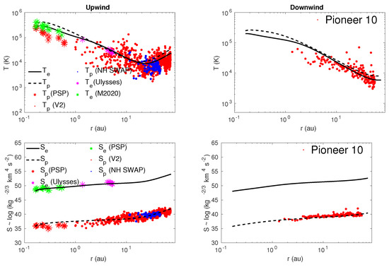
Figure 1.
Top left and right: Comparison between the theoretical and observed solar wind proton and electron temperatures as a function of heliocentric distance in the upwind and downwind directions. Bottom left and right: Comparison between the theoretical and observed proton and electron entropy as a function of heliocentric distance in the upwind and downwind directions. The solid and dashed curves show the solar wind proton and electron temperature, respectively. The red and green “*” symbols indicate the proton and electron (M2020) Moncuquet et al. [119] temperatures measured by PSP in the outbound direction during its first encounter. The magenta “*” indicates the electron temperature measured by . The red “.” symbols on the left and right panels indicate the proton temperatures measured by 2 and 10, respectively. The blue “.” indicates the proton temperature measured by NH SWAP.
In the downwind direction (∼180), 10 shows no significant or obvious increase in proton temperature (red “.” symbols in the top right panel of Figure 1), unlike the 2 measurements in the upwind direction. As shown in Figure 1 in [118], the hydrogen distribution in a narrow conical region in the downwind direction is less than that in the upwind direction, leading to a reduced pickup ion number density and hence source of turbulence yielding a lower heating rate in the downwind direction compared to the upwind direction. The top right panel of Figure 1 shows that the theoretical proton temperature (dashed curve) decreases gradually with increasing heliocentric distance, similar to the proton temperature measured by 10. The electron temperature (solid curve) decreases more slowly than the proton temperature within ∼3–4 au. Electron and proton temperatures are almost flat beyond ∼50–60 au.
The bottom left and right panels of Figure 1 show the theoretical and observed proton and electron entropy as a function of heliocentric distance in the upwind and downwind directions, respectively. In the upwind direction, the theoretical and observed electron entropy increases as a function of heliocentric distance, which is about 12.48% higher at 75 au than at 0.17 au. Similarly, the theoretical and observed proton entropy increases monotonically with distance. The proton entropy increases by about 17.24% at 75 au from 0.17 au. In the downwind direction, the electron entropy increases by about 9.11% and the proton entropy by about 12.5% from 0.17 au.
The top left and right panels of Figure 2 show the energy in forward propagating modes as a function of heliocentric distance in the upwind and downwind directions, respectively. In the left panel, the theoretical energy in forward propagating modes is compared with and 2 measurements. In the right panel, the theoretical energy in forward propagating modes is compared with 10 measurements. The theoretical and observed results are in good agreement. Since the 10 magnetometer data are not available after 10 au, the observed energy in forward propagating modes is plotted over the distance 1–10 au. In the upwind direction, the theoretical energy in forward propagating modes tends to flatten after ∼10 au, while in the downwind direction, the theoretical energy in forward propagating modes is slightly flat after ∼50 au. Similarly, the theoretical energy in backward propagating modes is in good agreement with and 2 measurements in the upwind direction (Figure 2, the left panel of the second row) and 10 measurements in the downwind direction (Figure 2, the right panel of the second row). However, after ∼10 au and ∼30 au, the pickup ions begin to affect the theoretical energy in backward propagating modes in the upwind and downwind directions, respectively. The theoretical results of the energy in forward and backward propagating modes clearly show that the turbulence energy is different in the upwind and strictly downwind directions.
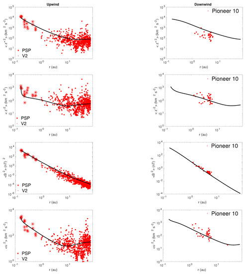
Figure 2.
From top to bottom in the upwind (left column) and downwind (—right column) directions, the theoretical and observed energy in forward propagating modes, energy in backward propagating modes, fluctuating magnetic energy, and fluctuating kinetic energy are compared as a function of heliocentric distance. The solid curve denotes the theoretical result. The red “*” symbols and “.” symbols represent and 2 measurements, respectively.
The theoretical fluctuating magnetic energy in the upwind direction (Figure 2, left panel of the third row) decreases as , while that in the downwind direction decreases as (Figure 2, right panel of the third row). Thus, turbulent magnetic energy in the downwind direction decreases faster than that in the upwind direction. The results show that the theoretical magnetic energy is in good agreement with the measured values of (red “*” symbols) and 2 (red “.” symbols) in the upwind direction, and the measured values of 10 (red “.” symbols) in the downwind direction. Similarly, in the upwind direction, the theoretical turbulent kinetic energy (bottom left panel of Figure 2) decreases gradually with increasing distance until ∼10 au, and then increases with distance. However, in the downwind direction, the theoretical turbulent kinetic energy decreases monotonically until ∼30–40 au, and then increases slightly with distance. The theoretical turbulent kinetic energy is in good agreement with the observed turbulent kinetic energy in the upwind and downwind directions.
The top left and right panels of Figure 3 plot the normalized residual energy as a function of heliocentric distance in the upwind and downwind directions. The theoretical normalized residual energy shows a similar radial profile to that of the observed normalized residual energy in both directions, although the scatter is large. The normalized residual energy in the downwind region does not tend towards equipartition between the fluctuating kinetic and magnetic energy with increasing distance, as in the upwind region. In the upwind direction, the fluctuations are increasingly magnetic dominated over the distance 2–10 au. Only after that does . This means that fluctuations in the upwind region beyond ∼10 au are more Alfvénic than that in the downwind region. The Alfvénicity of the solar wind in the outer heliosphere is due to wave excitation by the pickup ions. In the upwind direction (Figure 3, left panel of the second row), the theoretical normalized cross-helicity is high at the left boundary, decreases gradually as a function of heliocentric distance. In the downwind direction (Figure 3, right panel of the second row), the normalized cross-helicity is high at 0.17 au, and decreases gradually with increasing heliocentric distance. The theoretical normalized cross-helicity is in reasonable agreement with the observed normalized cross-helicity in the upwind direction, while the theoretical cross-helicity is greater than the observed cross-helicity in the downwind direction between 1 and 10 au. The bottom left and right panels of Figure 3 show the Alfvén ratio as a function of heliocentric distance in the upwind and downwind directions, respectively. The results show that the theoretical and observed Alfvén ratios are consistent.
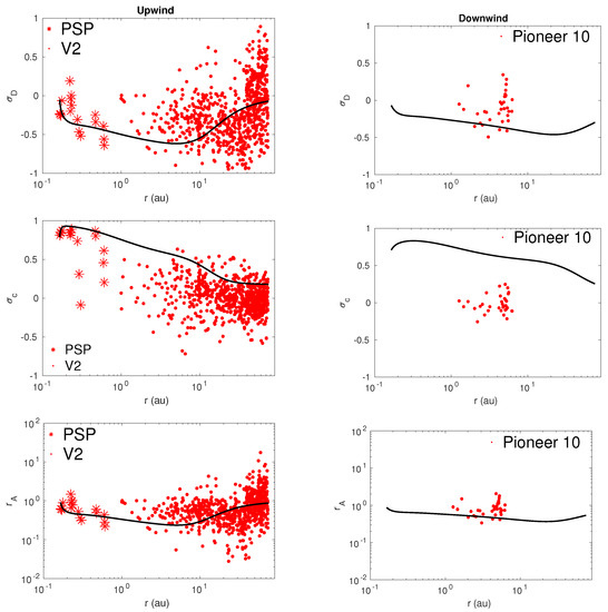
Figure 3.
From top to bottom in the upwind direction (left column) and the downwind direction (right column), the theoretical and observed normalized residual energy, normalized cross-helicity, and Alfvén ratio are compared as a function of heliocentric distance. The solid curves denote the theoretical results. The red “*” and “.” symbols represent the PSP and 2 measurements, respectively.
The correlation length is an important quantity because it determines the decay rate of turbulence, and hence controls the turbulent heating rate. The top left and right panels of Figure 4 show the correlation length corresponding to forward and backward propagating modes, and the residual energy as a function of heliocentric distance in the upwind and downwind directions. The theoretical correlation length corresponding to forward and backward propagating modes (the red and blue curves on the left panel, respectively) increases gradually with distance until ∼10 au, and then remains approximately constant with increasing heliocentric distance. Since the pickup ions excite Alfvén waves in the outer heliosphere beyond the ionization cavity, this leads to an increase in turbulent energy, which results in a flattening or a decrease of the correlation length through the adjustment of the Kolmogorov dissipation rate. The correlation length corresponding to forward and backward propagating modes (the red and blue curves on the left panel) in the downwind direction increases gradually until ∼40 au, and then remains approximately constant until ∼75 au. The correlation length of the residual energy (the green curves on the left and right panels) increases gradually as a function of heliocentric distance in the upwind and downwind directions.
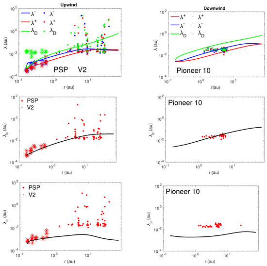
Figure 4.
From top to bottom in the upwind direction (left column) and downwind direction (right column), the theoretical and observed correlation lengths corresponding to forward and backward propagating modes and the residual energy (top panel), correlation length of magnetic field fluctuations (middle panel), and correlation length of fluctuating kinetic energy (bottom panel) are compared as a function of heliocentric distance, respectively. The solid curve denotes the theoretical correlation length. In the left column, the red, blue, and green “*” and “.” symbols represent the and 2 measurements, respectively. In the right panel, the red, blue, and green “.” symbol represents the 10 measurements.
The middle left and right panels of Figure 4 show the theoretical and observed correlation length of the magnetic field fluctuations in the upwind and downwind directions, respectively. The theoretical correlation length is in reasonable agreement with the observed . The bottom left and right panels show the comparison between the theoretical and observed correlation length of the velocity fluctuations as a function of heliocentric distance. In the upwind direction (left panel), the theoretical correlation length is in good agreement with the observed of PSP measurements, but does not agree with 2 measurements. Similarly, in the downwind direction, the theoretical does not agree with 10 measurements.
5. Turbulence Cascade in the Inertial Range throughout the Heliosphere
The turbulent cascade rate is directly related to the heating of the solar wind. Several authors have studied the turbulence cascade via observations [121,122,123,124,125,126,127], global MHD simulation [93], turbulence transport theory [34,103,128], and remote sensing observations [129,130,131]. These studies find that the turbulent heating rate is high near the Sun, and decreases with increasing heliocentric distance.
Vasquez et al. [121] used ACE measurements to examine the turbulence cascade as a function of proton temperature and solar wind speed. They argued that the cascade rate cannot be estimated with a Kolmogorov form, and better agreement is found when using an Irosnikov–Kraichnan form. However, Bandyopadhyay et al. [126] using PSP measurements showed that the cascade rate calculated from the Politano–Pouquet third-order law [132,133] and a von-Kármán phenomenology, which follows a Kolmogorov form, are approximately similar. Smith et al [123] studied the cascade rate of the energy in forward propagating modes, the total turbulent energy, and the cross-helicity from the third-order moments of the velocity and magnetic field fluctuations, finding that the cascade rate strongly depends on the correlation between the velocity and magnetic field fluctuations. Recently, Pine et al. [127] used the expression from Vasquez et al. [121], the turbulence transport theory, and wave excitation by newborn interstellar ions to study the turbulence cascade rate using 1 and 2 magnetometer data. They found that the first two expressions are very consistent, and the latter becomes important beyond 10 au. Their results also support idea that the heating of the solar wind plasma for au is mainly accomplished by turbulence of a solar origin, while the heating for au seems to be almost entirely due to the wave excitation by interstellar PUIs.
Using density modulation indices obtained using angular broadening observations of the Crab Nebula from 1952 to 2013, Sasikumar Raja et al. [131] calculated the solar wind proton heating rate using erg cms [129,134]. They found that the heating rate varies from to erg cm s over a distance R. Similarly, Ingale [135] also found that the heating rate varies between erg cm s over a heliocentric distance R. Using the coupled quasi-2D and NI/slab turbulence transport model equations [78], Adhikari et al. [128] found that the heating rate associated with quasi-2D turbulence is dominant. The heating rate corresponding to quasi-2D turbulence is erg cm s between R, and that of NI/slab turbulence is erg cm s between R.
Here, we derive the turbulence cascade rate for the energy in forward and backward propagating modes, the total turbulent energy, the cross-helicity, the residual energy, the fluctuating kinetic energy, and the fluctuating magnetic energy from two perspectives: (i) turbulence transport theory Zank et al. [77] (hereafter, called model 1), and (ii) a dimensional analysis between the power spectrum in the energy-containing range and the inertial range Adhikari et al. [136] (hereafter, called model 2). We first discuss the turbulence cascade rate via turbulence transport theory. The turbulence transport Equations (5)–(9) or (10)–(13) are derived without considering the viscous term. However, in deriving the turbulence transport model, the implicit assumption is that the inertial range of the turbulence spectrum is self-similar to the energy input rate in the inertial range, thus balancing the dissipation rate. This indicates that the energy transfer rate in the turbulence model is determined by the nonlinear term, which determines the heating of the solar wind plasma. Although turbulence transport modeling is a theory describing the transport of energy-containing range fluctuations, the decay of these fluctuations follows a Kolmogorov or Iroshnikov–Kraichnan (I–K) phenomenology. Therefore, the turbulence transport model calculates the balanced rate at which energy enters and exits the inertial range. It is found observationally that magnetic field fluctuations exhibit either a Kolmogorov or I–K type of power law in the inertial range [60,61,137,138,139,140,141,142].
The nonlinear term acts as a dissipative source for coronal and solar wind heating. The first term on the rhs of Equations (10) and (11) determines the cascade of the energy in forward and backward propagating modes, and the residual energy. These terms can be expressed as
where the denote the turbulence cascade rate of energy in forward/backward propagating modes, and the turbulence cascade rate of the residual energy. The parameter is a von Kármán–Taylor constant, and we choose [126]. Since the rhs term is positive in the Equation, the energy in forward and backward propagating modes always shows a forward cascade. However, for the turbulent cascade of the residual energy, there occurs a forward cascade for , and a reverse cascade for . Similarly, the turbulence cascade corresponding to the turbulent kinetic energy , the turbulent magnetic energy , the total turbulent energy , the (normalized) cross-helicity () , and the normalized residual energy can be written as
where the superscript “1” refers to model 1 derived from turbulence transport theory. Similar to the residual energy, the cross-helicity also shows a forward cascade when , and a reverse cascade when .
The second approach is based on the use of a dimensional analysis [136] to derive the turbulence cascade rate. Figure 5 is a schematic diagram, illustrating the power spectral density (PSD) of Elsässer energies , turbulent magnetic energy density , and the turbulent kinetic energy as a function of wavenumber k, where defines the power spectrum in the energy-containing range, and the power spectrum in the inertial range. The parameter A needs to be determined, is a Kolmogorov constant, and is the turbulence cascade rate. The wavenumber separates the energy-containing range and the inertial range. Since the PSD in the energy-containing range is equal to the PSD in the inertial range at , we can write
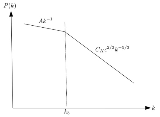
Figure 5.
Schematic diagram of the power spectral density of Elsässer energies , turbulent magnetic energy density , and the turbulent kinetic energy as a function of wavenumber k, illustrating the energy-containing range and the inertial range. The parameter is a spectral break wavenumber, which separates the energy-containing range and the inertial range.
Integrating the PSD from to yields
where we assume that km, which is equivalent to a solar rotation of ∼27 days [136]. The denominator on the rhs of Equation (25) is dimensionless, and the numerator has the dimension of energy, implying that the parameter A has the dimension of energy. From Equations (24) and (25), we obtain the turbulence cascade rate as,
Equation (26) calculates the turbulent cascade rate through the inertial range, which is derived by assuming that the solar wind fluctuations exhibit a Kolmogorov-like power law, and , where is the correlation length corresponding to the turbulent energy E.
We use Equation (26) to calculate the turbulence cascade of the fluctuating magnetic energy density , the energy in forward/backward propagating modes , and the turbulent kinetic energy . The turbulence cascade rates are given by
The turbulence cascade rate of the total turbulent energy, the (normalized) cross-helicity are given by,
where the superscript “2” refers to model 2 derived from the dimensional analysis.
Results: Turbulence Cascade in the Upwind and Downwind Directions
In this section, we discuss the upwind and downwind turbulence cascade rates from the perihelion of the first orbit of to 75 au. Figure 6 shows the turbulence cascade rate as a function of heliocentric distance in the upwind and downwind directions. In the figure, the solid line denotes the turbulence cascade rate calculated from model 1, i.e., based on turbulence transport theory, and the dashed line the turbulence cascade rate obtained from model 2, i.e., based on dimensional analysis. The red and blue curves represent the turbulence cascade rate in the downwind and upwind directions, respectively. Panels (a–d) of Figure 6 show the turbulence cascade rate of energy in forward propagating modes, energy in backward propagating modes, turbulent magnetic energy density, and the turbulent kinetic energy, respectively. The results show that the turbulence cascade rate in the downwind direction is higher than that in the upwind direction between ∼0.3 and ∼10–20 au. After ∼10–20 au, the turbulence cascade rate in the upwind direction is larger than that in the downwind direction because more turbulence is generated by pickup ions in the upwind direction than in the downwind direction. In the upwind direction, the turbulence cascade rate corresponding to energy in forward/backward propagating modes , fluctuating magnetic energy density , and fluctuating kinetic energy decreases with increasing heliocentric distance until au, and then increases or flatten with distance. In the downwind direction, the turbulence cascade rates of and decrease as distance increases until ∼40 au, and then flattens or decreases slightly with increasing distance. Models 1 and 2 reproduce similar turbulence cascade rates of , and in the upwind and downwind directions. For the turbulence cascade rate of , model 2 produces a larger rate than that of model 1. This is because the turbulence cascade rate in model 2 is inversely proportional to the correlation length, and the correlation length of velocity fluctuations is smaller in the outer heliosphere, yielding a higher turbulence cascade rate .
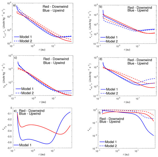
Figure 6.
The turbulence cascade rate as a function of heliocentric distance. Panels (a–f) show the turbulence cascade of the energy in forward propagating mode, the energy in backward propagating mode, turbulent kinetic energy, normalized cross-helicity, normalized residual energy, and turbulent magnetic energy density as a function of heliocentric distance, respectively. The blue and red curves denote the turbulence cascade in the upwind and downwind directions, respectively. The solid and dashed curves represent the turbulence cascade calculated by models 1, and 2, respectively.
Panel (e) of Figure 6 shows the turbulence cascade rate of the normalized residual energy as a function of heliocentric distance. The in the downwind direction (solid and dashed red curves) is larger than that in the upwind direction (solid and dashed blue curves) from 0.17 au to 20 au, and then it reverses. Model 1 produces a negative throughout the heliosphere, indicating that the turbulence cascade rate of the residual energy exhibits a reverse cascade within the inertial range. We note that the dimensional analysis is predicated on a particular form of the inertial range which is unlikely to be satisfied by a quantity that cannot be described by I-K theory. There is no theory for the residual energy analogous to Kolmogorov and so there is no reason to assume that the energy into the inertial range is balanced by the dissipation rate. Therefore, we only show the result of model 1.
Panel (f) of Figure 6 displays the turbulence cascade rate of normalized cross-helicity as a function of heliocentric distance. In the outer heliosphere, the in the upwind region is smaller than that in the downwind region because is approximately zero beyond ∼20 au in the upwind region, but not in the downwind region (see the middle right panel of Figure 3).
6. Cosmic Ray Diffusion Tensor throughout the Heliosphere
The propagation of cosmic ray (CR) is affected by low-frequency turbulence throughout the heliosphere [41,42,43,44,45,143,144,145,146]. The power in the magnetic fluctuations and the magnetic correlation length are responsible for the scattering of the CR [147].
A detailed understanding of the evolution of magnetic turbulence is required to calculate the parallel, perpendicular and drift components of the CR diffusion tensor. To calculate the perpendicular and drift components, the quantity needs to be evaluated, where is the particle gyrofrequency and an effective scattering time. It is generally believed that the magnetic field line wandering is the main physical mechanism that controls . There are two ways to model the magnetic field line wandering: quasi-linear theory (QLT) [147,148,149,150,151], and a nonperturbative approach [152,153,154,155,156].
QLT is a widely accepted theory to describe particle transport in a medium typically comprised of magnetized waves and/or fluctuations. In the case of purely 2D magnetic turbulence, QLT produces an infinitely large parallel diffusion since the pitch angle Fokker–Planck coefficient [150,151]. The basic principle of QLT is to assume that the charged particle gyro-orbits are weakly perturbed by electromagnetic fluctuations. One can evaluate the diffusion coefficient by expanding the terms of the Vlasov or collisionless Boltzmann equation into mean and fluctuating fields [157]. Matthaeus et al. [158] proposed a nonlinear guiding center (NLGC) theory for the perpendicular diffusion of charged particles, including the effect of parallel scattering and dynamical turbulence, finding good agreement between theory and simulation. Inspired by the success of NLGC theory, Shalchi et al. [159] proposed a weakly nonlinear theory (WNLT) for the parallel and perpendicular diffusion of CRs. In WNLT, the nonlinear effect produces a resonance broadening, which allows charged particles to scatter through [159]. The pitch-angle Fokker–Planck coefficient is no longer zero at and, therefore, yields a reasonable parallel diffusion length [160,161]. However, due to the complexity of the extended nonlinear theories for an ab initio turbulence model, we use a simple QLT description to describe the parallel diffusion of energetic charged particles [41].
For the perpendicular diffusion of energetic charged particles, we use the NLGC theory [158]. If turbulence is assumed to be entirely slab [162,163] or if the Kubo number [164] of the turbulence is small [165], the original NLGC theory produces inaccurate results. There are more sophisticated extensions of NLGC theory [166,167,168]. Shalchi [166] introduced an important extensions of NLGC theory, namely the unified nonlinear theory (UNLT), which addresses the weaknesses of NLGC theory. Turbulence responsible for the scattering of charged particles can be described as the superposition of a dominant 2D component and a minority slab component [41,43,44,154,155,156], in which case UNLT theory and NLGC theory give very similar results. If the turbulence models do not contain a dominant 2D component, the UNLT theory should be used instead of NLGC theory. In this work, we use a 3D incompressible MHD transport model to describe but to mimic the anisotropic character of solar wind turbulence, we decompose the magnetic energy density into a quasi-2D and a slab component in the ratio 80:20, i.e., 2D turbulence energy ), and slab turbulence energy ). Theory and observations predict that the ratio between the 2D and slab turbulence energy is 80:20 [62,103,169,170]. Similarly, we assume to calculate the 2D () and slab () magnetic correlation length, where is the magnetic correlation length. Zhao et al. [43,44] have used a NI MHD turbulence model Zank et al. [78] to investigate the CR diffusion tensor throughout the heliosphere. The WKB model for Alfvén waves was used originally to study the radial and latitudinal dependence of the CR diffusion tensor [171,172].
In CR modulation studies, the drift effect caused by the turbulent magnetic field is often ignored, and a drift coefficient derived under the assumption of weak scattering is adopted [173,174,175]. However, theoretical and simulation results show that the drift coefficient decreases in the presence of turbulence [176,177]. The famous classical scattering limit uses the parallel mfp and gyro-radius to calculate the reduction factor in the drift coefficient [149,178]. Zhao et al. [43] derived an expression for the drift velocity in a strong turbulence, in which the reduction factor is similar to that proposed by Tautz et al. [163], and the first order approach proposed by Engelbrecht et al. [175,179].
Zhao et al. [44] showed observationally that the CR parallel, perpendicular, and radial mean free paths are influenced by solar cycle at 1 au, and throughout the heliopshere [180]. Moloto et al. [181] developed a 3D time-dependent ab initio CR modulation model by using time-dependent large-scale quantities such as the magnetic field, tilt angle, solar wind speed, turbulent magnetic energy and the correlation length of the magnetic field fluctuations, finding reasonable agreement with spacecraft measurements, and reproduced the major salient features of the observed CR intensity temporal profile [175,182,183].
6.1. Cosmic Ray Diffusion Tensor
The CR diffusion tensor
describes the scattering of CRs by fluctuations in the heliospheric magnetic field. The parameters , , are the magnetic field components, is the Kronecker delta tensor, and is the alternating or Levi–Civita tensor. Here, and are the diagonal components of the CR diffusion tensor and describe diffusion along and perpendicular to the magnetic field, respectively. The diffusion term is an off-diagonal antisymmetric component that describes the particle drift caused by large-scale curvature and gradients in the IMF. The magnetic field is given by Equation (24) [106].
For solar modulation models, the radial diffusion coefficient is given by
where is the winding angle between the mean magnetic field and the radial direction,
Here, is the colatitude with respect to the solar axis rotation. We discuss the diffusion tensor in terms of the diffusion length scales , where v is the particle speed [41,43,44,184].
6.2. CR Parallel Mean Free Path
Bieber et al. [185] calculated the mfp considering the superposition of the 2D component and a minority slab component, and found that the mfp of electrons and protons is consistent with the Palmer consensus [186]. However, the restriction of solar wind turbulence to a purely slab model [147], yielded CR mfps that exceeded the Palmer consensus [185]. This suggests that the superposition of a majority 2D component and a minority slab component needs to be considered to calculate the mfp. The geometric structure of turbulence comprising a superposition of a dominant 2D and a minority slab component turbulence proposed by Bieber et al. [185] is consistent with the theoretical prediction of Zank et al. [169,187] and the observational results of Bieber et al. [170]. Theoretical and observational studies show that about 80% of the turbulence energy resides in the dominant 2D turbulence, and about 20% of the turbulence energy resides in the minority slab turbulence [169,170,187]. The parallel mfp based on the standard QLT and assuming magnetostatic turbulence is approximately [41],
where
The parameter , where p is the momentum, c is the speed of light, is the particle charge) is the particle rigidity, B is the magnetic field strength, is the particle Larmor radius, and is the variance of the x component of the slab fluctuations, and is assumed to be . Equation (32) is very close to the exact Fokker–Planck form. However, we note that expression (32) may not be fully accurate for very small rigidities when dynamical MHD turbulence is important [41,185]. The fractional term inside the squared brackets is particularly important in the outer heliosphere when the Larmor radius can be equal to or larger than the slab correlation length . In this case, the ions no longer resonate with the turbulent MHD fluctuations in the inertial range, but resonate with fluctuations in the energy-containing range. As a result, the scaling of relative to the rigidity P and the correlation length changes from the inner to outer heliosphere according to the variation of the correlation length with heliocentric distance.
6.3. CR Perpendicular Mean Free Path
There are different methods to calculate the perpendicular mfp . One method is to use the hard sphere scattering approach based on a relaxation time approximation [188,189,190]. The other method was developed by Bieber and Matthaeus [191] using the Green–Kubo–Taylor formula. This is different from the QLT, and underestimates the diffusion at low energy. We use the NLGC theory for the perpendicular diffusion, which was first proposed by Matthaeus et al. [158]. The NLGC theory assumes that the perpendicular diffusion is controlled by the velocity of gyrocenters along the field line, which allows both the random walk of the field line and the parallel scattering of CRs along the magnetic field line to be incorporated simultaneously. We use the expression for the perpendicular mfp from the Zank et al. [192] analysis [150],
where is the coefficient corresponding to the gyrocenter velocity, which is numerically found to be ∼1/3, and is a constant related to the spectral index , where is the gamma function.
The 2D turbulence power spectrum behavior at the lowest wavenumber, i.e., the outer scale, has an important impact on the perpendicular diffusion coefficients of charged particles in the heliosphere [146,193,194], including galactic cosmic ray proton and electron intensities. Engelbrecht et al. [193] calculated the galactic cosmic ray electron intensities using the observed size of magnetic islands [195,196], and different outer scales [136,145], finding that galactic cosmic ray electron differential intensities above kinetic energy 0.1 GeV are closer to the observed electron differential intensities, and lower than that below 0.1 GeV. Similarly, Engelbrecht et al. [194] proposed a new method to calculate the perpendicular diffusion coefficients by using the random ballistic decorrelation interpretation of the NLGC theory proposed by Ruffolo et al. [197]. The results show that the strength and anisotropy of solar energetic particle (SEP) are very sensitive to the pitch-angle dependence of the perpendicular diffusion coefficient.
6.4. Results: CR mfp in the Upwind and Downwind Directions
Figure 7 shows the radial dependence of the parallel mfp (blue lines), perpendicular mfp (red lines), radial mfp (cyan lines), and (green lines) for a proton with rigidity 445 MV (equivalent to 100 MeV proton) in the upwind direction (the solid line) and the downwind direction (the dashed line). In the upwind and downwind directions, the parallel mfp increases as a function of heliocentric distance. From 0.17 au to ∼0.3 au, in the upwind direction is smaller than that in the downwind direction, and then reverses from ∼0.3 au to ∼10 au, after which in the downwind direction becomes larger than that in the upwind region. At 75 au, the parallel mfp in the downwind direction is about 2 times greater than that in the upwind direction.
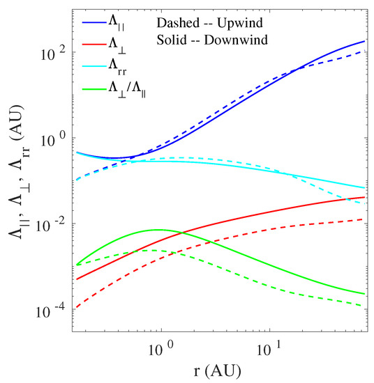
Figure 7.
The radial evolution of the CR parallel (blue lines), perpendicular (red lines), and radial (cyan lines) mean free path for a proton with rigidity of 445 MV for an outwardly directed IMF. It is assumed that the ratio of 2D fluctuating magnetic energy to slab fluctuating magnetic energy is 80:20 and . The radial evolution of the fluctuating magnetic energy and the correlation length of magnetic field fluctuations are shown in the third row of Figure 2 and the middle panel of Figure 4, respectively.
In the upwind and downwind directions, the perpendicular mfp increases gradually as a function of heliocentric distance. The perpendicular mfp in the downwind direction is about five times larger than that in the upwind direction throughout the heliosphere. The radial mfp in the upwind direction is less than that in the downwind direction between 0.17 au and 0.3 au, and then reverses between 0.3 au and 10 au, after which in the downwind region is about three to five times greater than that in the upwind direction.
The results show that the ratio of the perpendicular to parallel mfp in the upwind direction increases gradually from 0.17 au to au, and then decreases monotonically with increasing heliocentric distance. Similarly, in the upwind direction, the ratio increases slowly from 0.17 au to 1 au, and then decreases gradually as a function of heliocentric distance. The result shows that the parallel mfp dominates the perpendicular mfp in the upwind and downwind directions throughout the heliosphere. The radial trends for the parallel, perpendicular, and radial mfps are similar with those of Zhao et al. [43,44].
7. Discussion and Conclusions
We developed a 1D steady-state turbulence model, including the separate dissipation of turbulence energy in proton and electron heating, that incorporated the electron heat flux and Coulomb collisions between solar wind protons and electrons. We solved the coupled turbulence transport model equations from 0.17 to 75 au in the upwind and downwind directions. In the upwind direction, we compared the theoretical results with , 2, and measurements, and with 10 measurements in the downwind direction. Since the 10 magnetometer data are not available beyond 10 au, the observed quantities are plotted from 1 to 10 au in the downwind direction. We found reasonable agreement between the theoretical and observed results.
We derived expressions for the turbulence cascade rates for the energy in forward and backward propagating modes, total turbulent energy, normalized residual energy, normalized cross-helicity, fluctuating kinetic and magnetic energy from two perspectives: (i) a turbulence transport theory Zank et al. [77] (model 1), and (ii) a dimensional analysis between the power spectrum in the energy containing range and the inertial range Adhikari et al. [136] (model 2). Models 1 and 2 yield similar turbulence cascade rates for the energy in forward and backward propagating modes, magnetic energy density, and the normalized cross-helicity in the upwind and downwind directions. Finally, we calculated the CR diffusion tensor in the upwind and downwind directions. Our basic conclusions can be summarized using three categories.
A. Electron and proton heating in the upwind and downwind directions conclusions:
- Turbulence heats solar wind electrons and protons differently in the upwind and downwind directions. The proton and electron temperatures increase beyond ∼20 au in the upwind direction, but not in the downwind direction. The Coulomb collisions between protons and electrons, and the electron heat flux affect the radial profile of electron and proton temperatures but the effect of Coulomb collision is negligible compared to the turbulent heating term.
- The theoretical and observed electron and proton entropy increase as a function of heliocentric distance. In the upwind direction, the electron and proton entropy increases by about 12.48% and 17.24% from 0.17 au to 75 au, respectively. In the downwind direction from 0.17 to 75 au, the electron entropy increases by about 9.11% and the proton entropy by about 12.5%. The entropy in the upwind direction is higher than that in the downwind direction.
- In the upwind direction, the theoretical and observed energy in forward and backward propagating modes decreases gradually until ∼10–20 au, and then slightly increases as distance increases. In the downwind direction, the theoretical energy in forward and backward propagating modes decreases monotonically until ∼40–50 au, and then slightly increases until 75 au.
- The fluctuating magnetic energy density in the upwind direction decreases as , while that in the downwind direction decreases as . Similarly, in the upwind direction, the fluctuating kinetic energy decreases gradually until ∼10 au, and then increases as distance increases. However, in the downwind direction, the fluctuating kinetic energy decreases monotonically until ∼40 au, and then increases as a function of heliocentric distance.
- In the upwind direction, the fluctuating kinetic and magnetic energies tend towards equipartition beyond ∼10 au. In the downwind direction, the normalized residual energy increases after ∼30 au, but the fluctuating magnetic and kinetic energy do not balance. The normalized cross-helicity in the upwind direction is approximately zero beyond ∼20 au, but not in the downwind direction.
B. Turbulence cascade rate in the upwind and downwind directions:
- The turbulence cascade rate of energy in forward and backward propagating modes and the fluctuating magnetic energy decrease gradually until ∼10 au and ∼40 au in the upwind and downwind directions, respectively, and then increases slightly with increasing heliocentric distance.
- Over the heliocentric distance ∼0.2–10 au, the downwind turbulence cascade rate is larger than the upwind turbulence cascade rate. However, the turbulence cascade rate in the upwind direction is larger than that in the downwind direction beyond 10 au when pickup ions begin to influence the solar wind.
- The turbulence cascade rate of the normalized residual energy obtained from model 1 is negative throughout the heliosphere in the upwind and downwind directions.
- The turbulence cascade rate of the normalized cross-helicity in the downwind direction is larger than that in the upwind direction.
C. CR mfps in the upwind and downwind directions:
- The cosmic ray parallel mfp dominates the perpendicular mfp throughout the heliosphere in the upwind and downwind directions. The CR parallel mfp in the upwind direction is larger than that in the downwind direction between ∼0.2–10 au. The CR parallel mfp in the downwind direction is larger than that in the upwind direction when pickup ions begin to influence the solar wind.
- The CR perpendicular mfp increases monotonically as a function of heliocentric distance in the upwind and downwind directions. In the downwind direction, the CR perpendicular mfp is larger than that in the upwind direction from 0.17 au to 75 au.
- In the upwind direction, the CR radial mfp increases initially until ∼1–2 au, and then decreases gradually until ∼10 au. When pickup ions begin to affect the solar wind beyond ∼10 au, the decreases more rapidly. In the downwind direction, remains approximately constant between ∼0.1–10 au, and then decreases with increasing heliocentric distance.
We studied solar wind turbulence in the upwind and downwind directions in detail by using an incompressible MHD turbulence transport model [77] and spacecraft measurements. The results show that solar wind turbulence characterized by turbulence energies and correlation lengths, is different in the upwind than downwind direction. The different turbulence properties in the upwind and downwind directions yield different turbulence cascade rates and CR diffusion tensors in these two directions. The latter point is of particular importance to models describing cosmic ray modulation since typically the CR diffusion tensor has been assumed to be the same in both the upwind and downwind directions. Thus, besides the difference in the upwind and downwind distances to the heliospheric termination shock e.g., refs. [94,198], the character of the turbulence and hence CR scattering mfps is different.
Author Contributions
Conceptualization, L.A., G.P.Z.; Formal analysis, L.A., G.P.Z., L.Z.; Writing—original draft, L.A.; Writing—review and editing, L.A., G.P.Z., L.Z. All authors have read and agreed to the published version of the manuscript.
Funding
We acknowledge the partial support of a Parker Solar Probe contract SV4-84017, a NASA award 80NSSC20K1783, and an NSF EPSCoR RII-Track-1 cooperative agreement OIA-1655280. The SWEAP Investigation and this study are supported by the PSP mission under NASA contract NNN06AA01C.
Data Availability Statement
The Parker Solar Probe (), , 2, and 10 magnetometer and plasma data were obtained from the NASA CDAWeb website.
Conflicts of Interest
The authors declare no conflict of interest.
References
- Gazis, P.R.; Barnes, A.; Mihalov, J.D.; Lazarus, A.J. Solar wind velocity and temperature in the outer heliosphere. J. Geophys. Res. 1994, 99, 6561–6573. [Google Scholar] [CrossRef]
- Freeman, J.W. Estimates of solar wind heating inside 0.3 AU. Geophys. Res. Lett. 1988, 15, 88–91. [Google Scholar] [CrossRef]
- Williams, L.L.; Zank, G.P.; Matthaeus, W.H. Dissipation of pickup-induced waves: A solar wind temperature increase in the outer heliosphere? J. Geophys. Res. 1995, 100, 17059–17068. [Google Scholar] [CrossRef]
- Matthaeus, W.H.; Zank, G.P.; Smith, C.W.; Oughton, S. Turbulence, Spatial Transport, and Heating of the Solar Wind. Phys. Rev. Lett. 1999, 82, 3444–3447. [Google Scholar] [CrossRef]
- Smith, C.W.; Matthaeus, W.H.; Zank, G.P.; Ness, N.F.; Oughton, S.; Richardson, J.D. Heating of the low-latitude solar wind by dissipation of turbulent magnetic fluctuations. J. Geophys. Res. 2001, 106, 8253–8272. [Google Scholar] [CrossRef]
- Smith, C.W.; Isenberg, P.A.; Matthaeus, W.H.; Richardson, J.D. Turbulent Heating of the Solar Wind by Newborn Interstellar Pickup Protons. ApJ 2006, 638, 508–517. [Google Scholar] [CrossRef]
- Smith, C.W.; Vasquez, B.J.; Hamilton, K. Interplanetary magnetic fluctuation anisotropy in the inertial range. J. Geophys. Res. Space Phys. 2006, 111, 9111. [Google Scholar] [CrossRef]
- Isenberg, P.A.; Smith, C.W.; Matthaeus, W.H. Turbulent Heating of the Distant Solar Wind by Interstellar Pickup Protons. ApJ 2003, 592, 564–573. [Google Scholar] [CrossRef]
- Isenberg, P.A. Turbulence-driven Solar Wind Heating and Energization of Pickup Protons in the Outer Heliosphere. ApJ 2005, 623, 502–510. [Google Scholar] [CrossRef]
- Breech, B.; Matthaeus, W.H.; Minnie, J.; Bieber, J.W.; Oughton, S.; Smith, C.W.; Isenberg, P.A. Turbulence transport throughout the heliosphere. J. Geophys. Res. Space Phys. 2008, 113, 8105. [Google Scholar] [CrossRef]
- Breech, B.; Matthaeus, W.H.; Cranmer, S.R.; Kasper, J.C.; Oughton, S. Electron and proton heating by solar wind turbulence. J. Geophys. Res. Space Phys. 2009, 114, A09103. [Google Scholar] [CrossRef]
- Isenberg, P.A.; Smith, C.W.; Matthaeus, W.H.; Richardson, J.D. Turbulent Heating of the Distant Solar Wind by Interstellar Pickup Protons in a Decelerating Flow. ApJ 2010, 719, 716–721. [Google Scholar] [CrossRef]
- Ng, C.S.; Bhattacharjee, A.; Munsi, D.; Isenberg, P.A.; Smith, C.W. Kolmogorov versus Iroshnikov-Kraichnan spectra: Consequences for ion heating in the solar wind. J. Geophys. Res. Space Phys. 2010, 115, 2101. [Google Scholar] [CrossRef]
- Usmanov, A.V.; Matthaeus, W.H.; Breech, B.A.; Goldstein, M.L. Solar Wind Modeling with Turbulence Transport and Heating. ApJ 2011, 727, 84. [Google Scholar] [CrossRef]
- Oughton, S.; Matthaeus, W.H.; Smith, C.W.; Breech, B.; Isenberg, P.A. Transport of solar wind fluctuations: A two-component model. J. Geophys. Res. Space Phys. 2011, 116, 8105. [Google Scholar] [CrossRef]
- Adhikari, L.; Zank, G.P.; Hu, Q.; Dosch, A. Turbulence Transport Modeling of the Temporal Outer Heliosphere. ApJ 2014, 793, 52. [Google Scholar] [CrossRef]
- Adhikari, L.; Zank, G.P.; Bruno, R.; Telloni, D.; Hunana, P.; Dosch, A.; Marino, R.; Hu, Q. The Transport of Low-frequency Turbulence in Astrophysical Flows. II. Solutions for the Super-Alfvénic Solar Wind. ApJ 2015, 805, 63. [Google Scholar] [CrossRef]
- Adhikari, L.; Zank, G.P.; Hunana, P.; Shiota, D.; Bruno, R.; Hu, Q.; Telloni, D., II. Transport of Nearly Incompressible Magnetohydrodynamic Turbulence from 1 to 75 au. ApJ 2017, 841, 85. [Google Scholar] [CrossRef]
- Adhikari, L.; Zank, G.P.; Zhao, L.L.; Kasper, J.C.; Korreck, K.E.; Stevens, M.; Case, A.W.; Whittlesey, P.; Larson, D.; Livi, R.; et al. Turbulence Transport Modeling and First Orbit Parker Solar Probe (PSP) Observations. ApJ Suppl. 2020, 246, 38. [Google Scholar] [CrossRef]
- Adhikari, L.; Zank, G.P.; Zhao, L.L.; Webb, G.M. Evolution of Entropy and Mediation of the Solar Wind by Turbulence. ApJ 2020, 891, 34. [Google Scholar] [CrossRef]
- Wiengarten, T.; Fichtner, H.; Kleimann, J.; Kissmann, R. Implementing Turbulence Transport in the CRONOS Framework and Application to the Propagation of CMEs. ApJ 2015, 805, 155. [Google Scholar] [CrossRef]
- Wiengarten, T.; Oughton, S.; Engelbrecht, N.E.; Fichtner, H.; Kleimann, J.; Scherer, K. A Generalized Two-component Model of Solar Wind Turbulence and ab initio Diffusion Mean-Free Paths and Drift Lengthscales of Cosmic Rays. ApJ 2016, 833, 17. [Google Scholar] [CrossRef]
- Zank, G.P.; Adhikari, L.; Zhao, L.L.; Mostafavi, P.; Zirnstein, E.J.; McComas, D.J. The Pickup Ion-mediated Solar Wind. ApJ 2018, 869, 23. [Google Scholar] [CrossRef]
- Li, G.; Zank, G.P.; Rice, W.K.M. Energetic particle acceleration and transport at coronal mass ejection-driven shocks. J. Geophys. Res. Space Phys. 2003, 108, 1082. [Google Scholar] [CrossRef]
- Zank, G.P.; Li, G.; Verkhoglyadova, O. Particle Acceleration at Interplanetary Shocks. Space Sci. Rev. 2007, 130, 255–272. [Google Scholar] [CrossRef]
- Leer, E.; Holzer, T.E.; Fla, T. Acceleration of the solar wind. Space Sci. Rev. 1982, 33, 161–200. [Google Scholar] [CrossRef]
- Matthaeus, W.H.; Zank, G.P.; Oughton, S.; Mullan, D.J.; Dmitruk, P. Coronal Heating by Magnetohydrodynamic Turbulence Driven by Reflected Low-Frequency Waves. ApJ Lett. 1999, 523, L93–L96. [Google Scholar] [CrossRef]
- Oughton, S.; Matthaeus, W.H.; Dmitruk, P.; Milano, L.J.; Zank, G.P.; Mullan, D.J. A Reduced Magnetohydrodynamic Model of Coronal Heating in Open Magnetic Regions Driven by Reflected Low-Frequency Alfvén Waves. ApJ 2001, 551, 565–575. [Google Scholar] [CrossRef]
- Dmitruk, P.; Milano, L.J.; Matthaeus, W.H. Wave-driven Turbulent Coronal Heating in Open Field Line Regions: Nonlinear Phenomenological Model. ApJ 2001, 548, 482–491. [Google Scholar] [CrossRef]
- Dmitruk, P.; Matthaeus, W.H.; Milano, L.J.; Oughton, S.; Zank, G.P.; Mullan, D.J. Coronal Heating Distribution Due to Low-Frequency, Wave-driven Turbulence. ApJ 2002, 575, 571–577. [Google Scholar] [CrossRef]
- Suzuki, T.K.; Inutsuka, S.I. Making the Corona and the Fast Solar Wind: A Self-consistent Simulation for the Low-Frequency Alfvén Waves from the Photosphere to 0.3 AU. ApJ Lett. 2005, 632, L49–L52. [Google Scholar] [CrossRef]
- Suzuki, T.K.; Inutsuka, S.I. Solar winds driven by nonlinear low-frequency Alfvén waves from the photosphere: Parametric study for fast/slow winds and disappearance of solar winds. J. Geophys. Res. Space Phys. 2006, 111, 6101. [Google Scholar] [CrossRef]
- Cranmer, S.R.; van Ballegooijen, A.A.; Edgar, R.J. Self-consistent Coronal Heating and Solar Wind Acceleration from Anisotropic Magnetohydrodynamic Turbulence. ApJ Suppl. 2007, 171, 520–551. [Google Scholar] [CrossRef]
- Verdini, A.; Velli, M.; Matthaeus, W.H.; Oughton, S.; Dmitruk, P. A Turbulence-Driven Model for Heating and Acceleration of the Fast Wind in Coronal Holes. ApJ Lett. 2010, 708, L116–L120. [Google Scholar] [CrossRef]
- van Ballegooijen, A.A.; Asgari-Targhi, M.; Cranmer, S.R.; DeLuca, E.E. Heating of the Solar Chromosphere and Corona by Alfvén Wave Turbulence. ApJ 2011, 736, 3. [Google Scholar] [CrossRef]
- van Ballegooijen, A.A.; Asgari-Targhi, M. Heating and Acceleration of the Fast Solar Wind by Alfvén Wave Turbulence. ApJ 2016, 821, 106. [Google Scholar] [CrossRef]
- Lionello, R.; Velli, M.; Downs, C.; Linker, J.A.; Mikić, Z.; Verdini, A. Validating a Time-dependent Turbulence-driven Model of the Solar Wind. ApJ 2014, 784, 120. [Google Scholar] [CrossRef]
- Asgari-Targhi, M.; van Ballegooijen, A.A.; Cranmer, S.R.; DeLuca, E.E. The Spatial and Temporal Dependence of Coronal Heating by Alfvén Wave Turbulence. ApJ 2013, 773, 111. [Google Scholar] [CrossRef]
- Matsumoto, T.; Suzuki, T.K. Connecting the Sun and the solar wind: The self-consistent transition of heating mechanisms. MNRAS 2014, 440, 971–986. [Google Scholar] [CrossRef]
- Zank, G.P.; Adhikari, L.; Hunana, P.; Tiwari, S.K.; Moore, R.; Shiota, D.; Bruno, R.; Telloni, D. Theory and Transport of Nearly Incompressible Magnetohydrodynamic Turbulence. IV. Solar Coronal Turbulence. ApJ 2018, 854, 32. [Google Scholar] [CrossRef]
- Zank, G.P.; Matthaeus, W.H.; Bieber, J.W.; Moraal, H. The radial and latitudinal dependence of the cosmic ray diffusion tensor in the heliosphere. J. Geophys. Res. 1998, 103, 2085. [Google Scholar] [CrossRef]
- Florinski, V.; Zank, G.P.; Pogorelov, N.V. Galactic cosmic ray transport in the global heliosphere. J. Geophys. Res. Space Phys. 2003, 108, 1228. [Google Scholar] [CrossRef]
- Zhao, L.L.; Adhikari, L.; Zank, G.P.; Hu, Q.; Feng, X.S. Cosmic Ray Diffusion Tensor throughout the Heliosphere Derived from a Nearly Incompressible Magnetohydrodynamic Turbulence Model. ApJ 2017, 849, 88. [Google Scholar] [CrossRef]
- Zhao, L.L.; Adhikari, L.; Zank, G.P.; Hu, Q.; Feng, X.S. Influence of the Solar Cycle on Turbulence Properties and Cosmic-Ray Diffusion. ApJ 2018, 856, 94. [Google Scholar] [CrossRef]
- Chhiber, R.; Subedi, P.; Usmanov, A.V.; Matthaeus, W.H.; Ruffolo, D.; Goldstein, M.L.; Parashar, T.N. Cosmic-Ray Diffusion Coefficients throughout the Inner Heliosphere from a Global Solar Wind Simulation. ApJ Suppl. 2017, 230, 21. [Google Scholar] [CrossRef]
- Adhikari, L.; Zank, G.P.; Zhao, L.L.; Webb, G.M. Evolution of entropy in the outer heliosphere. J. Phys. Conf. Ser. 2020, 1620, 012001. [Google Scholar] [CrossRef]
- Adhikari, L.; Zank, G.P.; Zhao, L.L.; Nakanotani, M.; Tasnim, S. Modeling proton and electron heating in the fast solar wind. Astron. Astrophys. 2021, 650, A16. [Google Scholar] [CrossRef]
- Coleman, P., Jr. J. Turbulence, Viscosity, and Dissipation in the Solar-Wind Plasma. ApJ 1968, 153, 371. [Google Scholar] [CrossRef]
- Belcher, J.W.; Davis, L., Jr.; Smith, E.J. Large-amplitude Alfvén waves in the interplanetary medium: Mariner 5. J. Geophys. Res. 1969, 74, 2302. [Google Scholar] [CrossRef]
- Belcher, J.W.; Davis, L., Jr. Large-amplitude Alfvén waves in the interplanetary medium, 2. J. Geophys. Res. 1971, 76, 3534. [Google Scholar] [CrossRef]
- Bavassano, B.; Dobrowolny, M.; Mariani, F.; Ness, N.F. Radial evolution of power spectra of interplanetary Alfvenic turbulence. J. Geophys. Res. 1982, 87, 3617–3622. [Google Scholar] [CrossRef]
- Bavassano, B.; Pietropaolo, E.; Bruno, R. Cross-helicity and residual energy in solar wind turbulence—Radial evolution and latitudinal dependence in the region from 1 to 5 AU. J. Geophys. Res. 1998, 103, 6521. [Google Scholar] [CrossRef]
- Bavassano, B.; Pietropaolo, E.; Bruno, R. Radial evolution of outward and inward Alfvénic fluctuations in the solar wind: A comparison between equatorial and polar observations by Ulysses. J. Geophys. Res. 2001, 106, 10659–10668. [Google Scholar] [CrossRef]
- Roberts, D.A.; Goldstein, M.L.; Klein, L.W.; Matthaeus, W.H. Origin and evolution of fluctuations in the solar wind—HELIOS observations and Helios-Voyager comparisons. J. Geophys. Res. 1987, 92, 12023–12035. [Google Scholar] [CrossRef]
- Roberts, D.A.; Klein, L.W.; Goldstein, M.L.; Matthaeus, W.H. The nature and evolution of magnetohydrodynamic fluctuations in the solar wind—Voyager observations. J. Geophys. Res. 1987, 92, 11021–11040. [Google Scholar] [CrossRef]
- Goldstein, B.E.; Smith, E.J.; Balogh, A.; Horbury, T.S.; Goldstein, M.L.; Roberts, D.A. Properties of magnetohydrodynamic turbulence in the solar wind as observed by Ulysses at high heliographic latitudes. Geophys. Res. Lett. 1995, 22, 3393–3396. [Google Scholar] [CrossRef]
- Tu, C.Y.; Marsch, E. MHD structures, waves and turbulence in the solar wind: Observations and theories. Space Sci. Rev. 1995, 73, 1–210. [Google Scholar] [CrossRef]
- Kolmogorov, A. The Local Structure of Turbulence in Incompressible Viscous Fluid for Very Large Reynolds’ Numbers. Akad. Nauk SSSR Dokl. 1941, 30, 301–305. [Google Scholar]
- Kraichnan, R.H. Inertial-Range Spectrum of Hydromagnetic Turbulence. Phys. Fluids 1965, 8, 1385–1387. [Google Scholar] [CrossRef]
- Telloni, D.; Carbone, F.; Bruno, R.; Sorriso-Valvo, L.; Zank, G.P.; Adhikari, L.; Hunana, P. No Evidence for Critical Balance in Field-aligned Alfvénic Solar Wind Turbulence. ApJ 2019, 887, 160. [Google Scholar] [CrossRef]
- Zhao, L.L.; Zank, G.P.; Adhikari, L.; Nakanotani, M.; Telloni, D.; Carbone, F. Spectral Features in Field-aligned Solar Wind Turbulence from Parker Solar Probe Observations. ApJ 2020, 898, 113. [Google Scholar] [CrossRef]
- Zank, G.P.; Nakanotani, M.; Zhao, L.L.; Adhikari, L.; Telloni, D. Spectral Anisotropy in 2D plus Slab Magnetohydrodynamic Turbulence in the Solar Wind and Upper Corona. ApJ 2020, 900, 115. [Google Scholar] [CrossRef]
- Tu, C.Y.; Pu, Z.Y.; Wei, F.S. The power spectrum of interplanetary Alfvénic fluctuations: Derivation of the governing equation and its solution. J. Geophys. Res. 1984, 89, 9695–9702. [Google Scholar] [CrossRef]
- Adhikari, L.; Zank, G.P.; Bruno, R.; Telloni, D.; Hunana, P.; Dosch, A.; Marino, R.; Hu, Q. The transport of low-frequency turbulence in the super-Alfvénic solar wind. J. Phys. Conf. Ser. 2015, 642, 012001. [Google Scholar] [CrossRef]
- Parker, E.N. Dynamical Theory of the Solar Wind. Space Sci. Rev. 1965, 4, 666–708. [Google Scholar] [CrossRef]
- Whang, Y.C. Alfvén waves in spiral interplanetary field. J. Geophys. Res. 1973, 78, 7221. [Google Scholar] [CrossRef]
- Hollweg, J.V. Alfvén Waves in a Two-Fluid Model of the Solar Wind. ApJ 1973, 181, 547–566. [Google Scholar] [CrossRef]
- Hollweg, J.V. Alfvén waves in the solar wind: Wave pressure, poynting flux, and angular momentum. J. Geophys. Res. 1973, 78, 3643. [Google Scholar] [CrossRef]
- Barnes, A.; Hollweg, J.V. Large-amplitude hydromagnetic waves. J. Geophys. Res. 1974, 79, 2302. [Google Scholar] [CrossRef]
- Iroshnikov, P.S. Turbulence of a Conducting Fluid in a Strong Magnetic Field. Soviet Ast. 1964, 7, 566. [Google Scholar]
- Goldreich, P.; Sridhar, S. Toward a theory of interstellar turbulence. 2: Strong alfvenic turbulence. ApJ 1995, 438, 763–775. [Google Scholar] [CrossRef]
- Elsässer, W.M. The Hydromagnetic Equations. Phys. Rev. 1950, 79, 183. [Google Scholar] [CrossRef]
- Zhou, Y.; Matthaeus, W.H. Models of inertial range spectra of interplanetary magnetohydrodynamic turbulence. J. Geophys. Res. 1990, 95, 14881–14892. [Google Scholar] [CrossRef]
- Zhou, Y.; Matthaeus, W.H. Remarks on transport theories of interplanetary fluctuations. J. Geophys. Res. 1990, 95, 14863–14871. [Google Scholar] [CrossRef]
- Marsch, E.; Tu, C.Y. Dynamics of correlation functions with Elsasser variables for inhomogeneous MHD turbulence. J. Plasma Phys. 1989, 41, 479–491. [Google Scholar] [CrossRef]
- Zank, G.P.; Matthaeus, W.H.; Smith, C.W. Evolution of turbulent magnetic fluctuation power with heliospheric distance. J. Geophys. Res. 1996, 101, 17093–17108. [Google Scholar] [CrossRef]
- Zank, G.P.; Dosch, A.; Hunana, P.; Florinski, V.; Matthaeus, W.H.; Webb, G.M. The Transport of Low-frequency Turbulence in Astrophysical Flows. I. Governing Equations. ApJ 2012, 745, 35. [Google Scholar] [CrossRef]
- Zank, G.P.; Adhikari, L.; Hunana, P.; Shiota, D.; Bruno, R.; Telloni, D. Theory and Transport of Nearly Incompressible Magnetohydrodynamic Turbulence. ApJ 2017, 835, 147. [Google Scholar] [CrossRef]
- Matthaeus, W.H.; Minnie, J.; Breech, B.; Parhi, S.; Bieber, J.W.; Oughton, S. Transport of cross helicity and radial evolution of Alfvénicity in the solar wind. Geophys. Res. Lett. 2004, 31, 12803. [Google Scholar] [CrossRef]
- Breech, B.; Matthaeus, W.H.; Minnie, J.; Oughton, S.; Parhi, S.; Bieber, J.W.; Bavassano, B. Radial evolution of cross helicity in high-latitude solar wind. Geophys. Res. Lett. 2005, 32, 6103. [Google Scholar] [CrossRef]
- von Karman, T.; Howarth, L. On the Statistical Theory of Isotropic Turbulence. R. Soc. Lond. Proc. Ser. A 1938, 164, 192–215. [Google Scholar] [CrossRef]
- Batchelor, G.K. The Theory of Homogeneous Turbulence; Cambridge University Press: Cambridge, MA, USA, 1953. [Google Scholar]
- Matthaeus, W.H.; Oughton, S.; Pontius, D.H., Jr.; Zhou, Y. Evolution of energy-containing turbulent eddies in the solar wind. J. Geophys. Res. 1994, 99, 19267. [Google Scholar] [CrossRef]
- Matthaeus, W.H.; Zank, G.P.; Oughton, S. Phenomenology of hydromagnetic turbulence in a uniformly expanding medium. J. Plasma Phys. 1996, 56, 659–675. [Google Scholar] [CrossRef]
- Dosch, A.; Adhikari, L.; Zank, G.P. The Transport of Low-Frequency Turbulence in Astrophysical Flows: Correlation Lengths; American Institute of Physics Conference Series; Zank, G.P., Borovsky, J., Bruno, R., Cirtain, J., Cranmer, S., Elliott, H., Giacalone, J., Gonzalez, W., Li, G., Marsch, E., et al., Eds.; American Institute of Physics: College Park, MD, USA, 2013; Volume 1539, pp. 155–158. [Google Scholar] [CrossRef]
- Hossain, M.; Gray, P.C.; Pontius, D.H., Jr.; Matthaeus, W.H.; Oughton, S. Phenomenology for the decay of energy-containing eddies in homogeneous MHD turbulence. Phys. Fluids 1995, 7, 2886–2904. [Google Scholar] [CrossRef]
- Usmanov, A.V.; Goldstein, M.L.; Matthaeus, W.H. Three-dimensional Magnetohydrodynamic Modeling of the Solar Wind Including Pickup Protons and Turbulence Transport. ApJ 2012, 754, 40. [Google Scholar] [CrossRef]
- Usmanov, A.V.; Goldstein, M.L.; Matthaeus, W.H. Three-fluid, Three-dimensional Magnetohydrodynamic Solar Wind Model with Eddy Viscosity and Turbulent Resistivity. ApJ 2014, 788, 43. [Google Scholar] [CrossRef]
- Usmanov, A.V.; Matthaeus, W.H.; Goldstein, M.L.; Chhiber, R. The Steady Global Corona and Solar Wind: A Three-dimensional MHD Simulation with Turbulence Transport and Heating. ApJ 2018, 865, 25. [Google Scholar] [CrossRef]
- Kryukov, I.A.; Pogorelov, N.V.; Zank, G.P.; Borovikov, S.N. Numerical modeling of the solar wind turbulence; American Institute of Physics Conference Series; Heerikhuisen, J., Li, G., Pogorelov, N., Zank, G., Eds.; American Institute of Physics: College Park, MD, USA, 2012; Volume 1436, pp. 48–54. [Google Scholar] [CrossRef]
- Shiota, D.; Zank, G.P.; Adhikari, L.; Hunana, P.; Telloni, D.; Bruno, R. Turbulent Transport in a Three-dimensional Solar Wind. ApJ 2017, 837, 75. [Google Scholar] [CrossRef]
- Chhiber, R.; Usmanov, A.V.; DeForest, C.E.; Matthaeus, W.H.; Parashar, T.N.; Goldstein, M.L. Weakened Magnetization and Onset of Large-scale Turbulence in the Young Solar Wind—Comparisons of Remote Sensing Observations with Simulation. ApJ Lett. 2018, 856, L39. [Google Scholar] [CrossRef]
- Chhiber, R.; Usmanov, A.V.; Matthaeus, W.H.; Parashar, T.N.; Goldstein, M.L. Contextual Predictions for Parker Solar Probe. II. Turbulence Properties and Taylor Hypothesis. ApJ Suppl. 2019, 242, 12. [Google Scholar] [CrossRef]
- Zank, G.P. Interaction of the solar wind with the local interstellar medium: A theoretical perspective. Space Sci. Rev. 1999, 89, 413–688. [Google Scholar] [CrossRef]
- Zank, G.P.; Pauls, H.L. Modelling the Heliosphere. Space Sci. Rev. 1996, 78, 95–106. [Google Scholar] [CrossRef]
- Rice, W.K.M.; Zank, G.P. Shock propagation in the outer heliosphere 3. Pickup ions, MHD, cosmic rays, and energetic particles. J. Geophys. Res. 2000, 105, 5157–5166. [Google Scholar] [CrossRef]
- Shiota, D.; Kataoka, R.; Miyoshi, Y.; Hara, T.; Tao, C.; Masunaga, K.; Futaana, Y.; Terada, N. Inner heliosphere MHD modeling system applicable to space weather forecasting for the other planets. Space Weather 2014, 12, 187–204. [Google Scholar] [CrossRef]
- Wang, Y.M.; Sheeley, N.R.J. Solar Wind Speed and Coronal Flux-Tube Expansion. ApJ 1990, 355, 726. [Google Scholar] [CrossRef]
- Arge, C.N.; Pizzo, V.J. Improvement in the prediction of solar wind conditions using near-real time solar magnetic field updates. J. Geophys. Res. 2000, 105, 10465–10480. [Google Scholar] [CrossRef]
- Leamon, R.J.; Matthaeus, W.H.; Smith, C.W.; Wong, H.K. Contribution of Cyclotron-resonant Damping to Kinetic Dissipation of Interplanetary Turbulence. ApJ Lett. 1998, 507, L181–L184. [Google Scholar] [CrossRef]
- Cranmer, S.R.; Matthaeus, W.H.; Breech, B.A.; Kasper, J.C. Empirical Constraints on Proton and Electron Heating in the Fast Solar Wind. ApJ 2009, 702, 1604–1614. [Google Scholar] [CrossRef]
- Engelbrecht, N.E.; Strauss, R.D.T. A Tractable Estimate for the Dissipation Range Onset Wavenumber Throughout the Heliosphere. ApJ 2018, 856, 159. [Google Scholar] [CrossRef]
- Zank, G.P.; Zhao, L.L.; Adhikari, L.; Telloni, D.; Kasper, J.C.; Bale, S.D. Turbulence transport in the solar corona: Theory, modeling, and Parker Solar Probe. Phys. Plasmas 2021, 28, 080501. [Google Scholar] [CrossRef]
- Boldyrev, S.; Forest, C.; Egedal, J. On the temperature of the solar wind. arXiv 2020, arXiv:2001.05125. [Google Scholar]
- Tang, B.; Zank, G.P.; Kolobov, V.I. Numerical Modeling of Suprathermal Electron Transport in the Solar Wind: Effects of Whistler Turbulence. ApJ 2020, 892, 95. [Google Scholar] [CrossRef]
- Weber, E.J.; Davis, L., Jr. The Angular Momentum of the Solar Wind. ApJ 1967, 148, 217–227. [Google Scholar] [CrossRef]
- Spitzer, L. Physics of Fully Ionized Gases. J. Am. Chem. Soc. 1962, 78, 19–5133. [Google Scholar] [CrossRef]
- Isenberg, P.A. Resonant acceleration and heating of solar wind ions: Anisotropy and dispersion. J. Geophys. Res. 1984, 89, 6613–6622. [Google Scholar] [CrossRef]
- Cranmer, S.R.; Field, G.B.; Kohl, J.L. Spectroscopic Constraints on Models of Ion Cyclotron Resonance Heating in the Polar Solar Corona and High-Speed Solar Wind. ApJ 1999, 518, 937–947. [Google Scholar] [CrossRef]
- Salem, C.; Hubert, D.; Lacombe, C.; Bale, S.D.; Mangeney, A.; Larson, D.E.; Lin, R.P. Electron Properties and Coulomb Collisions in the Solar Wind at 1 AU: Wind Observations. ApJ 2003, 585, 1147–1157. [Google Scholar] [CrossRef]
- Braginskii, S.I. Transport Processes in a Plasma. Rev. Plasma Phys. 1965, 1, 205. [Google Scholar]
- Spitzer, L.; Härm, R. Transport Phenomena in a Completely Ionized Gas. Phys. Rev. 1953, 89, 977–981. [Google Scholar] [CrossRef]
- Hollweg, J.V. Collisionless electron heat conduction in the solar wind. J. Geophys. Res. 1976, 81, 1649. [Google Scholar] [CrossRef]
- Scudder, J.D.; Olbert, S. A theory of local and global processes which affect solar wind electrons 1. The origin of typical 1 AU velocity distribution functions-steady state theory. J. Geophys. Res. 1979, 84, 2755–2772. [Google Scholar] [CrossRef]
- Pilipp, W.G.; Muehlhaeuser, K.H.; Miggenrieder, H.; Rosenbauer, H.; Schwenn, R. Large-scale variations of thermal electron parameters in the solar wind between 0.3 and 1 AU. J. Geophys. Res. 1990, 95, 6305–6329. [Google Scholar] [CrossRef]
- Howes, G.G. A prescription for the turbulent heating of astrophysical plasmas. MNRAS 2010, 409, L104–L108. [Google Scholar] [CrossRef]
- Howes, G.G. Prediction of the Proton-to-total Turbulent Heating in the Solar Wind. ApJ 2011, 738, 40. [Google Scholar] [CrossRef][Green Version]
- Nakanotani, M.; Zank, G.P.; Adhikari, L.; Zhao, L.L.; Giacalone, J.; Opher, M.; Richardson, J.D. The Downwind Solar Wind: Model Comparison with Pioneer 10 Observations. ApJ Lett. 2020, 901, L23. [Google Scholar] [CrossRef]
- Moncuquet, M.; Meyer-Vernet, N.; Issautier, K.; Pulupa, M.; Bonnell, J.W.; Bale, S.D.; Dudok de Wit, T.; Goetz, K.; Griton, L.; Harvey, P.R.; et al. First In Situ Measurements of Electron Density and Temperature from Quasi-thermal Noise Spectroscopy with Parker Solar Probe/FIELDS. ApJ Supp. 2020, 246, 44. [Google Scholar] [CrossRef]
- McComas, D.J.; Bame, S.J.; Barraclough, B.L.; Feldman, W.C.; Funsten, H.O.; Gosling, J.T.; Riley, P.; Skoug, R.; Balogh, A.; Forsyth, R.; et al. Ulysses’ return to the slow solar wind. Geophys. Res. Lett. 1998, 25, 1–4. [Google Scholar] [CrossRef]
- Vasquez, B.J.; Smith, C.W.; Hamilton, K.; MacBride, B.T.; Leamon, R.J. Evaluation of the turbulent energy cascade rates from the upper inertial range in the solar wind at 1 AU. J. Geophys. Res. 2007, 112, A07101. [Google Scholar] [CrossRef]
- MacBride, B.T.; Smith, C.W.; Forman, M.A. The Turbulent Cascade at 1 AU: Energy Transfer and the Third-Order Scaling for MHD. ApJ 2008, 679, 1644–1660. [Google Scholar] [CrossRef]
- Smith, C.W.; Stawarz, J.E.; Vasquez, B.J.; Forman, M.A.; MacBride, B.T. Turbulent Cascade at 1 AU in High Cross-Helicity Flows. Phys. Rev. Lett. 2009, 103, 201101. [Google Scholar] [CrossRef] [PubMed]
- Podesta, J.J. On the energy cascade rate of solar wind turbulence in high cross helicity flows. J. Geophys. Res. Space Phys. 2011, 116, A05101. [Google Scholar] [CrossRef]
- Bandyopadhyay, R.; Chasapis, A.; Chhiber, R.; Parashar, T.N.; Maruca, B.A.; Matthaeus, W.H.; Schwartz, S.J.; Eriksson, S.; Le Contel, O.; Breuillard, H.; et al. Solar Wind Turbulence Studies Using MMS Fast Plasma Investigation Data. ApJ 2018, 866, 81. [Google Scholar] [CrossRef]
- Bandyopadhyay, R.; Goldstein, M.L.; Maruca, B.A.; Matthaeus, W.H.; Parashar, T.N.; Ruffolo, D.; Chhiber, R.; Usmanov, A.; Chasapis, A.; Qudsi, R.; et al. Enhanced Energy Transfer Rate in Solar Wind Turbulence Observed near the Sun from Parker Solar Probe. ApJ Suppl. 2020, 246, 48. [Google Scholar] [CrossRef]
- Pine, Z.B.; Smith, C.W.; Hollick, S.J.; Argall, M.R.; Vasquez, B.J.; Isenberg, P.A.; Schwadron, N.A.; Joyce, C.J.; Sokół, J.M.; Bzowski, M.; et al. Turbulent Transport and Heating of the Solar Wind Using Voyager Observations. ApJ 2020, 900, 94. [Google Scholar] [CrossRef]
- Adhikari, L.; Zank, G.P.; Zhao, L.L. A Solar Coronal Hole and Fast Solar Wind Turbulence Model and First-orbit Parker Solar Probe (PSP) Observations. ApJ 2020, 901, 102. [Google Scholar] [CrossRef]
- Chandran, B.D.G.; Quataert, E.; Howes, G.G.; Xia, Q.; Pongkitiwanichakul, P. Constraining Low-Frequency Alfvénic Turbulence in the Solar Wind Using Density-Fluctuation Measurements. ApJ 2009, 707, 1668–1675. [Google Scholar] [CrossRef]
- Cranmer, S.R. Heating Rates for Protons and Electrons in Polar Coronal Holes: Empirical Constraints from the Ultraviolet Coronagraph Spectrometer. ApJ 2020, 900, 105. [Google Scholar] [CrossRef]
- Sasikumar Raja, K.; Subramanian, P.; Ingale, M.; Ramesh, R.; Maksimovic, M. Turbulent Proton Heating Rate in the Solar Wind from 5 to 45 R⊙. ApJ 2021, 914, 137. [Google Scholar] [CrossRef]
- Politano, H.; Pouquet, A. Dynamical length scales for turbulent magnetized flows. Geophys. Res. Lett. 1998, 25, 273–276. [Google Scholar] [CrossRef]
- Politano, H.; Pouquet, A. von Kármán-Howarth equation for magnetohydrodynamics and its consequences on third-order longitudinal structure and correlation functions. PhRvE 1998, 57, R21–R24. [Google Scholar] [CrossRef]
- Hollweg, J.V. Kinetic Alfvén wave revisited. J. Geophys. Res. 1999, 104, 14811–14820. [Google Scholar] [CrossRef]
- Ingale, M. Turbulent density fluctuations in the solar wind. arXiv 2015, arXiv:1509.07652. [Google Scholar]
- Adhikari, L.; Zank, G.P.; Telloni, D.; Hunana, P.; Bruno, R.; Shiota, D. Theory and Transport of Nearly Incompressible Magnetohydrodynamics Turbulence. III. Evolution of Power Anistropy in Magnetic Field Fluctuations throughout the Heliosphere. ApJ 2017, 851, 117. [Google Scholar] [CrossRef]
- Horbury, T.S.; Forman, M.; Oughton, S. Anisotropic Scaling of Magnetohydrodynamic Turbulence. Phys. Rev. Lett. 2008, 101, 175005. [Google Scholar] [CrossRef] [PubMed]
- Podesta, J.J.; Roberts, D.A.; Goldstein, M.L. Spectral Exponents of Kinetic and Magnetic Energy Spectra in Solar Wind Turbulence. ApJ 2007, 664, 543–548. [Google Scholar] [CrossRef]
- Wicks, R.T.; Horbury, T.S.; Chen, C.H.K.; Schekochihin, A.A. Power and spectral index anisotropy of the entire inertial range of turbulence in the fast solar wind. MNRAS 2010, 407, L31–L35. [Google Scholar] [CrossRef]
- Bruno, R.; Telloni, D. Spectral Analysis of Magnetic Fluctuations at Proton Scales from Fast to Slow Solar Wind. ApJ Lett. 2015, 811, L17. [Google Scholar] [CrossRef]
- Chen, C.H.K.; Bale, S.D.; Bonnell, J.W.; Borovikov, D.; Bowen, T.A.; Burgess, D.; Case, A.W.; Chandran, B.D.G.; de Wit, T.D.; Goetz, K.; et al. The Evolution and Role of Solar Wind Turbulence in the Inner Heliosphere. ApJ Supp. 2020, 246, 53. [Google Scholar] [CrossRef]
- Pine, Z.B.; Smith, C.W.; Hollick, S.J.; Argall, M.R.; Vasquez, B.J.; Isenberg, P.A.; Schwadron, N.A.; Joyce, C.J.; Sokół, J.M.; Bzowski, M.; et al. Evidence for Dissipation of Magnetic Fluctuations Using Voyager and ACE Observations. ApJ 2020, 900, 91. [Google Scholar] [CrossRef]
- Pei, C.; Bieber, J.W.; Breech, B.; Burger, R.A.; Clem, J.; Matthaeus, W.H. Cosmic ray diffusion tensor throughout the heliosphere. J. Geophys. Res. Space Phys. 2010, 115, A03103. [Google Scholar] [CrossRef]
- Engelbrecht, N.E.; Burger, R.A. An Ab Initio Model for the Modulation of Galactic Cosmic-ray Electrons. ApJ 2013, 779, 158. [Google Scholar] [CrossRef]
- Engelbrecht, N.E.; Burger, R.A. An Ab Initio Model for Cosmic-ray Modulation. ApJ 2013, 772, 46. [Google Scholar] [CrossRef]
- Engelbrecht, N.E.; Burger, R.A. Sensitivity of Cosmic-Ray Proton Spectra to the Low-wavenumber Behavior of the 2D Turbulence Power Spectrum. ApJ 2015, 814, 152. [Google Scholar] [CrossRef]
- Jokipii, J.R. Cosmic-Ray Propagation. I. Charged Particles in a Random Magnetic Field. ApJ 1966, 146, 480. [Google Scholar] [CrossRef]
- Jokipii, J.R.; Parker, E.N. Random Walk of Magnetic Lines of Force in Astrophysics. Phys. Rev. Lett. 1968, 21, 44–47. [Google Scholar] [CrossRef]
- Forman, M.A.; Jokipii, J.R.; Owens, A.J. Cosmic-Ray Streaming Perpendicular to the Mean Magnetic Field. ApJ 1974, 192, 535–540. [Google Scholar] [CrossRef]
- Shalchi, A.; Bieber, J.W.; Matthaeus, W.H. Analytic Forms of the Perpendicular Diffusion Coefficient in Magnetostatic Turbulence. ApJ 2004, 604, 675–686. [Google Scholar] [CrossRef]
- Shalchi, A.; Schlickeiser, R. Cosmic ray transport in anisotropic magnetohydrodynamic turbulence. III. Mixed magnetosonic and Alfvénic turbulence. Astron. Astrophys. 2004, 420, 799–808. [Google Scholar] [CrossRef]
- Matthaeus, W.H.; Gray, P.C.; Pontius, D.H.J.; Bieber, J.W. Spatial Structure and Field-Line Diffusion in Transverse Magnetic Turbulence. Phys. Rev. Lett. 1995, 75, 2136–2139. [Google Scholar] [CrossRef] [PubMed]
- Gray, P.C.; Pontius, D.H.J.; Matthaeus, W.H. Scaling of field-line random walk in model solar wind fluctuations. Geophys. Res. Lett. 1996, 23, 965–968. [Google Scholar] [CrossRef]
- Shalchi, A.; Bieber, J.W.; Matthaeus, W.H.; Schlickeiser, R. Parallel and Perpendicular Transport of Heliospheric Cosmic Rays in an Improved Dynamical Turbulence Model. ApJ 2006, 642, 230–243. [Google Scholar] [CrossRef]
- Shalchi, A. Analytic forms of the cosmic ray perpendicular diffusion coefficient with implicit contribution of slab modes. Adv. Space Res. 2018, 62, 2817–2827. [Google Scholar] [CrossRef]
- Shalchi, A. Perpendicular Transport of Energetic Particles in Magnetic Turbulence. Space Sci. Rev. 2020, 216, 23. [Google Scholar] [CrossRef]
- Zank, G.P. Transport Processes in Space Physics and Astrophysics; Lecture Notes in Physics; Springer: Berlin, Germany, 2014; Volume 877. [Google Scholar] [CrossRef]
- Matthaeus, W.H.; Qin, G.; Bieber, J.W.; Zank, G.P. Nonlinear Collisionless Perpendicular Diffusion of Charged Particles. ApJ Lett. 2003, 590, L53–L56. [Google Scholar] [CrossRef]
- Shalchi, A.; Bieber, J.W.; Matthaeus, W.H.; Qin, G. Nonlinear Parallel and Perpendicular Diffusion of Charged Cosmic Rays in Weak Turbulence. ApJ 2004, 616, 617–629. [Google Scholar] [CrossRef]
- Shalchi, A. Second-order quasilinear theory of cosmic ray transport. Phys. Plasmas 2005, 12, 052905. [Google Scholar] [CrossRef]
- Shalchi, A. Nonlinear Cosmic Ray Diffusion Theories; Springer: Berlin/Heidelberg, Germany, 2009; Volume 362. [Google Scholar] [CrossRef]
- Jones, F.C.; Jokipii, J.R.; Baring, M.G. Charged-Particle Motion in Electromagnetic Fields Having at Least One Ignorable Spatial Coordinate. ApJ 1998, 509, 238–243. [Google Scholar] [CrossRef]
- Tautz, R.C.; Shalchi, A. Drift Coefficients of Charged Particles in Turbulent Magnetic Fields. ApJ 2012, 744, 125. [Google Scholar] [CrossRef]
- Kubo, R. Statistical-Mechanical Theory of Irreversible Processes. I. J. Phys. Soc. Jpn. 1957, 12, 570–586. [Google Scholar] [CrossRef]
- Shalchi, A. Extended nonlinear guiding center theory of perpendicular diffusion. Astron. Astrophys. 2006, 453, L43–L46. [Google Scholar] [CrossRef]
- Shalchi, A. A Unified Particle Diffusion Theory for Cross-field Scattering: Subdiffusion, Recovery of Diffusion, and Diffusion in Three-dimensional Turbulence. ApJ Lett. 2010, 720, L127–L130. [Google Scholar] [CrossRef]
- Shalchi, A. Simple Analytical Forms of the Perpendicular Diffusion Coefficient for Two-component Turbulence. I. Magnetostatic Turbulence. ApJ 2013, 774, 7. [Google Scholar] [CrossRef][Green Version]
- Shalchi, A. Simple Analytical Forms of the Perpendicular Diffusion Coefficient for Two-component Turbulence. II. Dynamical Turbulence with Constant Correlation Time. ApJ 2014, 780, 138. [Google Scholar] [CrossRef]
- Zank, G.P.; Matthaeus, W.H. Waves and turbulence in the solar wind. J. Geophys. Res. 1992, 97, 17189. [Google Scholar] [CrossRef]
- Bieber, J.W.; Wanner, W.; Matthaeus, W.H. Dominant two-dimensional solar wind turbulence with implications for cosmic ray transport. J. Geophys. Res. 1996, 101, 2511–2522. [Google Scholar] [CrossRef]
- Völk, H.J.; Morfill, G.; Alpers, W.; Lee, M.A. Spatial Dependence of the Pitch-Angle and Associated Spatial Diffusion Coefficients for Cosmic Rays in Interplanetary Space. Ap. & SS. 1974, 26, 403–430. [Google Scholar] [CrossRef]
- Morfill, G.E.; Völk, H.J. Latitude variation of interplanetary cosmic ray diffusion. J. Geophys. Res. 1979, 84, 4446–4450. [Google Scholar] [CrossRef]
- Zhang, M. A Markov Stochastic Process Theory of Cosmic-Ray Modulation. ApJ 1999, 513, 409–420. [Google Scholar] [CrossRef]
- Potgieter, M.S. Solar Modulation of Cosmic Rays. Living Rev. Sol. Phys. 2013, 10, 3. [Google Scholar] [CrossRef]
- Engelbrecht, N.E.; Moloto, K.D. An Ab Initio Approach to Antiproton Modulation in the Inner Heliosphere. ApJ 2021, 908, 167. [Google Scholar] [CrossRef]
- Candia, J.; Roulet, E. Diffusion and drift of cosmic rays in highly turbulent magnetic fields. J. Cosmol. Astropart. Phys. 2004, 2004, 007. [Google Scholar] [CrossRef]
- Burger, R.A.; Krüger, T.P.J.; Hitge, M.; Engelbrecht, N.E. A Fisk-Parker Hybrid Heliospheric Magnetic Field with a Solar-Cycle Dependence. ApJ 2008, 674, 511–519. [Google Scholar] [CrossRef]
- Jokipii, J.R.; Parker, E.N. on the Convection, Diffusion, and Adiabatic Deceleration of Cosmic Rays in the Solar Wind. ApJ 1970, 160, 735. [Google Scholar] [CrossRef]
- Engelbrecht, N.E.; Strauss, R.D.; le Roux, J.A.; Burger, R.A. Toward a Greater Understanding of the Reduction of Drift Coefficients in the Presence of Turbulence. ApJ 2017, 841, 107. [Google Scholar] [CrossRef]
- Zhao, L.L.; Qin, G.; Zhang, M.; Heber, B. Modulation of galactic cosmic rays during the unusual solar minimum between cycles 23 and 24. J. Geophys. Res. (Space Physics) 2014, 119, 1493–1506. [Google Scholar] [CrossRef]
- Moloto, K.D.; Engelbrecht, N.E. A Fully Time-dependent Ab Initio Cosmic-Ray Modulation Model Applied to Historical Cosmic-Ray Modulation. ApJ 2020, 894, 121. [Google Scholar] [CrossRef]
- Moloto, K.D.; Engelbrecht, N.E.; Burger, R.A. A Simplified Ab Initio Cosmic-ray Modulation Model with Simulated Time Dependence and Predictive Capability. ApJ 2018, 859, 107. [Google Scholar] [CrossRef]
- Moloto, K.D.; Engelbrecht, N.E.; Strauss, R.D.; Moeketsi, D.M.; van den Berg, J.P. Numerical integration of stochastic differential equations: A parallel cosmic ray modulation implementation on Africa’s fastest computer. Adv. Space Res. 2019, 63, 626–639. [Google Scholar] [CrossRef]
- Bieber, J.W.; Burger, R.A.; Matthaeus, W.H. The Diffusion Tensor throughout the Heliosphere. Int. Cosmic Ray Confer. 1995, 4, 694. [Google Scholar]
- Bieber, J.W.; Matthaeus, W.H.; Smith, C.W.; Wanner, W.; Kallenrode, M.B.; Wibberenz, G. Proton and Electron Mean Free Paths: The Palmer Consensus Revisited. ApJ 1994, 420, 294. [Google Scholar] [CrossRef]
- Palmer, I.D. Transport coefficients of low-energy cosmic rays in interplanetary space. Rev. Geophys. Space Phys. 1982, 20, 335–351. [Google Scholar] [CrossRef]
- Zank, G.P.; Matthaeus, W.H. Nearly incompressible fluids. II—Magnetohydrodynamics, turbulence, and waves. Phys. Fluids 1993, 5, 257–273. [Google Scholar] [CrossRef]
- Axford, W.I. The modulation of galactic cosmic rays in the interplanetary medium. Planet. Space Sci. 1965, 13, 115–130. [Google Scholar] [CrossRef]
- Gleeson, L.J.; Axford, W.I. Cosmic Rays in the Interplanetary Medium. ApJ Lett. 1967, 149, L115. [Google Scholar] [CrossRef]
- Jones, F.C. The Generalized Diffusion-Convection Equation. ApJ 1990, 361, 162. [Google Scholar] [CrossRef]
- Bieber, J.W.; Matthaeus, W.H. Perpendicular Diffusion and Drift at Intermediate Cosmic-Ray Energies. ApJ 1997, 485, 655–659. [Google Scholar] [CrossRef]
- Zank, G.P.; Li, G.; Florinski, V.; Matthaeus, W.H.; Webb, G.M.; Le Roux, J.A. Perpendicular diffusion coefficient for charged particles of arbitrary energy. J. Geophys. Res. Space Phys. 2004, 109, A04107. [Google Scholar] [CrossRef]
- Engelbrecht, N.E. The Implications of Simple Estimates of the 2D Outerscale Based on Measurements of Magnetic Islands for the Modulation of Galactic Cosmic-Ray Electrons. ApJ 2019, 872, 124. [Google Scholar] [CrossRef]
- Engelbrecht, N.E. On the Pitch-angle-dependent Perpendicular Diffusion Coefficients of Solar Energetic Protons in the Inner Heliosphere. ApJ 2019, 880, 60. [Google Scholar] [CrossRef]
- Khabarova, O.; Zank, G.P.; Li, G.; le Roux, J.A.; Webb, G.M.; Dosch, A.; Malandraki, O.E. Small-scale Magnetic Islands in the Solar Wind and Their Role in Particle Acceleration. I. Dynamics of Magnetic Islands Near the Heliospheric Current Sheet. ApJ 2015, 808, 181. [Google Scholar] [CrossRef]
- Cartwright, M.L.; Moldwin, M.B. Heliospheric evolution of solar wind small-scale magnetic flux ropes. J. Geophys. Res. Space Phys. 2010, 115, A08102. [Google Scholar] [CrossRef]
- Ruffolo, D.; Pianpanit, T.; Matthaeus, W.H.; Chuychai, P. Random Ballistic Interpretation of Nonlinear Guiding Center Theory. ApJ Lett. 2012, 747, L34. [Google Scholar] [CrossRef]
- Zank, G.P.; Hunana, P.; Mostafavi, P.; Le Roux, J.A.; Li, G.; Webb, G.M.; Khabarova, O.; Cummings, A.; Stone, E.; Decker, R. Diffusive Shock Acceleration and Reconnection Acceleration Processes. ApJ 2015, 814, 137. [Google Scholar] [CrossRef]


Publisher’s Note: MDPI stays neutral with regard to jurisdictional claims in published maps and institutional affiliations. |
© 2021 by the authors. Licensee MDPI, Basel, Switzerland. This article is an open access article distributed under the terms and conditions of the Creative Commons Attribution (CC BY) license (https://creativecommons.org/licenses/by/4.0/).