Article

Large-Eddy Simulation of a Hydrocyclone with an Air Core Using Two-Fluid and Volume-of-Fluid Models

1
Narmer-EngSim LLC, Blacksburg, VA 24060, USA
2
Department of Biomedical Engineering and Mechanics, Virginia Polytechnic Institute and State University, Blacksburg, VA 24061, USA
*
Author to whom correspondence should be addressed.
These authors contributed equally to this work.
Fluids 2021, 6(10), 364; https://doi.org/10.3390/fluids6100364
Submission received: 26 August 2021 / Revised: 23 September 2021 / Accepted: 28 September 2021 / Published: 14 October 2021
(This article belongs to the Special Issue Multiphase Flows in Engineering Applications)

Abstract

:
Large-eddy simulations have been conducted for two-phase flow (water and air) in a hydrocyclone using Two-Fluid (Euler–Euler) and Volume-of-Fluid (VOF) models. Subgrid stresses are modeled using a dynamic eddy–viscosity model, and results are compared to those using the Smagorinsky model. The effects of grid resolutions on the mean flow and turbulence statistics have been thoroughly investigated. Five block-structured grids of 0.72, 1.47, 2.4, 3.81, and 7.38 million elements have been used for the simulations of Hsieh’s 75 mm hydrocyclone Mean velocity profiles and normal Reynolds stresses have been compared with experimental data. Results of the two-fluid model are in good agreement with those of the VOF model. A fine mesh in the axial and radial directions is necessary for capturing the turbulent vortical structure. Turbulence structures in the hydrocyclone are dominated by helical vortices around the air core. Energy spectra are analyzed at different points in the hydrocyclone, and regions of low turbulent kinetic energy are identified and attributed to stabilizing effects of the swirling velocity component.

1. Introduction

Hydrocyclones are used in many industries for separation of different phases. In the mineral-processing industry, classifying hydrocyclones are used to classify ores after grinding based on their particle sizes ([1,2,3]). A typical geometry of classifying hydrocyclone consists of a cylindrical section followed by a conical section with two outlets that are open to the atmosphere. The top outlet is called the overflow opening and the bottom one is called the underflow opening. Slurry of water and solid particles is forced tangentially into the hydrocyclone top, and it swirls as it goes downward. The swirling flow field generates a column vortex with pressure decreasing radially towards the center. The strength of the vortex depends on the rate of input angular momentum about hydrocyclone centerline. The radial pressure gradient affects the motion of particles based on their specific gravity and/or sizes. Because of the low pressure created by the swirling layer of slurry, air enters through the underflow opening and forms an air core around the hydrocyclone centerline. The structure and motion of the air core depends on the operating conditions of the hydrocyclone ([4]). Hararah et al. [5] found that the distribution of tangential and axial velocity of air inside the core depends on the pressure drop and geometry of hydrocyclone. Devulapalli [6] experiments show that the inlet flow rate has a direct effect on the air core diameter.
Laboratory experiments and CFD techniques can be used for performance evaluation and improvements of hydrocyclones. Laboratory experiments are important to determine mean velocity profiles and turbulence statistics. However, such measurements are expensive and time consuming. The high cost of experiments limits their effectiveness to optimize the geometry of hydrocyclones. CFD techniques are viable tools to predict the flow structure and turbulence in hydrocyclones. Current computing capabilities enable conducting high fidelity numerical simulations such as Large-Eddy Simulation (LES) of two-phase flow in hydrocyclones at an affordable cost ([7,8,9,10,11,12]). However, validation of numerical models is an important step to assess their accuracy. In 1988, Hsieh [13] conducted both laboratory experiments and axisymmetric numerical simulations of flow in a hydrocyclone. His pioneering work shows good comparison between experimental velocity profiles and those from numerical simulations. However, the role of turbulence is essential in the flow behavior inside the swirling layer and air core. The experimental velocity profiles in Hsieh [13] show flow asymmetry. Therefore, 3D time-accurate simulations are essential to capture the spatial variations of the mean flow and instantaneous turbulence structures as those affect particles dispersion.
Structural stability of flow in hydrocyclones is achieved by feeding appropriate rate of angular momentum that drives the tangential and axial flow. The wall shear layers in the feeding duct become free shear layers upon entering the hydrocyclone volute. Instabilities on those layers produce new turbulence structures as the swirling flow go downward. The axial velocity distribution on the cross-section of hydrocyclone has a complex structure. Downward flow prevails near the outer cylindrical/conical walls whereas upward flow prevails near the interface with the air core. Local instabilities of such a complex shear flow produce turbulent vortical structures that continuously interact with a swirling flow. Because of the high tangential velocity of the swirling flow, the turbulent fluctuations in the tangential direction are not the same as those in the radial and axial directions indicating anisotropic large-scale turbulence. The nonlinear interaction between the mean flow and turbulent fluctuations affects the distribution of mean velocity components and hence the performance of a hydrocyclone. Therefore, it is important to use accurate turbulence models in numerical simulations. The first numerical approach to simulate turbulent flows is Unsteady Reynolds-Averaged Navier–Stokes (U-RANS) where ensemble-averaged equations are solved for mean flow and Reynolds stresses are modeled. Turbulence models of varying fidelity have been applied. Eddy–viscosity models such as 2-equation models k ϵ and k ω are well known. These models assume isotropic relations between local Reynolds stresses and the mean rate-of-strain tensor. Because of the flow structure in hydrocyclone, this isotropic condition in turbulent fluctuations is invalid. A more sophisticated turbulence model such as Reynolds Stress Transport Model (RSM) can be used to overcome the shortcomings in 2-equations turbulence models ([14,15,16,17,18]). In RSM, 6 transport equations are solved for Reynolds stress components and this shall increase computations time tremendously. The second approach is Large-Eddy simulation (LES) where the Navier–Stokes equations are space-filtered and solved on a fine grid to resolve large scales of turbulence [19]. The filter width is directly determined by the size of grid element. The effects of small scales of turbulence on the evolution and motion of large eddies are modeled by an eddy–viscosity subgrid stress model. Direct Numerical Simulations (DNS) approach is more accurate than LES where all the turbulent eddies down to Kolmogorov scale are resolved and turbulence modeling is not required. However, for industrial applications it is not feasible because of very large computational resources and time. Delgadillo and Rajamani ([14,15]), and Brennan ([16,17]) conducted two-phase LES and U-RANS simulations for Hsieh’s hydrocyclone [13]. They modeled the two-phase flow of air and water using Volume-Of-Fluid (VOF) and mixture models. Vakamalla and Mangadoddy [20] conducted a comprehensive study of the role of turbulence on mean velocity, turbulence statistics, and classification performance of different sizes of hydrocyclones. They tested different models in conjunction with VOF and mixture models. They demonstrated the superiority of LES approach over RSM for high turbulence hydrocyclones.
The mixture and VOF models are considered to be One-Fluid models where one set of momentum and continuity equations are solved in space and time. The air/water interface is reconstructed and tracked in VOF method by solving continuity equation for volume fraction of air phase. The experiments conducted by Hararah et al. [5] show that the air core destabilizes in the overflow pipe because of decrease in centrifugal forces and produces a mixture of air and water droplet (Aero-Suspension). The use of VOF approach is expensive in terms of computational resources and time to resolve this breakup and coalescence of water droplets and/or air bubbles in overflow pipe. The mixture model is computationally less demanding and simple where one set of momentum and continuity equations are solved for a homogeneous mixture of fluids phases. The slip velocity between dispersed phase and continuous phase is estimated by balancing drag and body force ([21]). The mixture model can be applied for a wide variety of turbulent multiphase flows where the response time is very small (i.e., very small inertia) relative to time scale of corresponding turbulent scales. In many applications of particulate and/or bubbly flows, the spatial distribution of dispersed phases cannot be accurately captured by a mixture model [22]. The interfacial momentum transfer in terms of drag, added mass and history forces between dispersed and continuous phases is the driving mechanism to suspend solid particles and/or distribute air bubbles in the liquid phase. Therefore, accurate modeling of interfacial phenomena is important to account for the effect of turbulent fluctuations on the motion of dispersed phases. The mixture multiphase model does not accurately model these interfacial forces. The Two-Fluid model is highly recommended as discussed by Ishii and Mishima [23]. In the Two-Fluid model we solve a set of averaged momentum and continuity equations for each of the phases. The motions of the phases are coupled by modeling interfacial forces such as drag, added mass, lift and history force. This approach of multiphase flows is more expensive than mixture model, but it is more accurate for multiphase problems that have large spatial variations in void fractions of dispersed phases. Moreover, the two-fluid model is the natural choice for air-sparged hydrocyclones ([24,25,26]) where there are a huge number of bubbles in addition to an air core or froth layer and resolving the gas-liquid interfaces is not computationally feasible by VOF.
This paper aims at validating the two-fluid model (Euler–Euler) for a hydrocyclone with an air core using LES by comparison with experimental data and simulation results using VOF model. Furthermore, a fine mesh of about 7.4 million elements for the 75 mm hydrocyclone designed by Hsieh [13] enables in-depth analysis of large-scale turbulence structures, statistics, and spectra. The influence of the subgrid-scale stresses model on the simulations results is evaluated. An eddy–viscosity model is used where the coefficient is determined by the dynamic model and the results are compared with predictions using Smagorinsky model. Validation of the LES in conjunction with the two-fluid model is important for future LES modeling of three-phase (gas-liquid-solid) in hydrocyclones and fluidized bed reactors [27].

2. Equations for Two-Fluid and VOF Models

2.1. Two-Fluid Model

The motion of the two continuous phases is described by the unsteady filtered Navier–Stokes equations:
Continuity equation:
( α i ρ i ) t + · ( α i ρ i V i ) = 0
Σ α i = 1
Momentum equation:
( α i ρ i V i ) t + · α i ρ i V i V i = α i P + α i ρ i g + · α i ρ i ν i + ν t V i + V i T + M i
where V i is the filtered velocity of phase i, P is the filtered pressure field which is shared by all phases, ρ i and α i are density and local volume fraction of phase i, respectively. g is the gravitational acceleration. The index (i = 1) denotes water phase and (i = 2) denotes air phase. The turbulent eddy viscosity ν t in the above equation is calculated as,
ν t = C m Δ 2 V i + V i T
The coefficient C m is known as the subgrid model constant. This coefficient is determined locally in the computational domain using Germano dynamic model [28]. For Smagorinsky model, the coefficient C m is replaced by a constant C s 2 . M i is the interfacial force that acts on phase (i) due to the presence of other phases. In the present simulations, momentum exchanges between the two phases due to drag and buoyancy on bubbles are the only mechanisms that couple the motion of the two phases. For the two-fluid model (Euler–Euler), a bubble diameter of 0.1 mm is assumed, while no such an assumption is needed with the VOF. Schiller-Naumann drag model [29] has been used to estimate drag coefficient of air bubbles.

2.2. Volume-of-Fluid Model

In the volume-of-fluid model (VOF) of two-phase flow, a single momentum equation is solved at every cell where density and viscosity are volume-weighted average of the density and viscosity of the two phases. Water is declared as the primary phase, and the air-water interface is tracked by solving the volume fraction equation of the air phase using a high-resolution scheme. Volume-weighted is used for smoothing the air-water interface. Brackbill et al. [30] Continuum Surface Force (CSF) model is used for the effects of surface tension. A constant surface tension of 0.07 N/m is assumed.

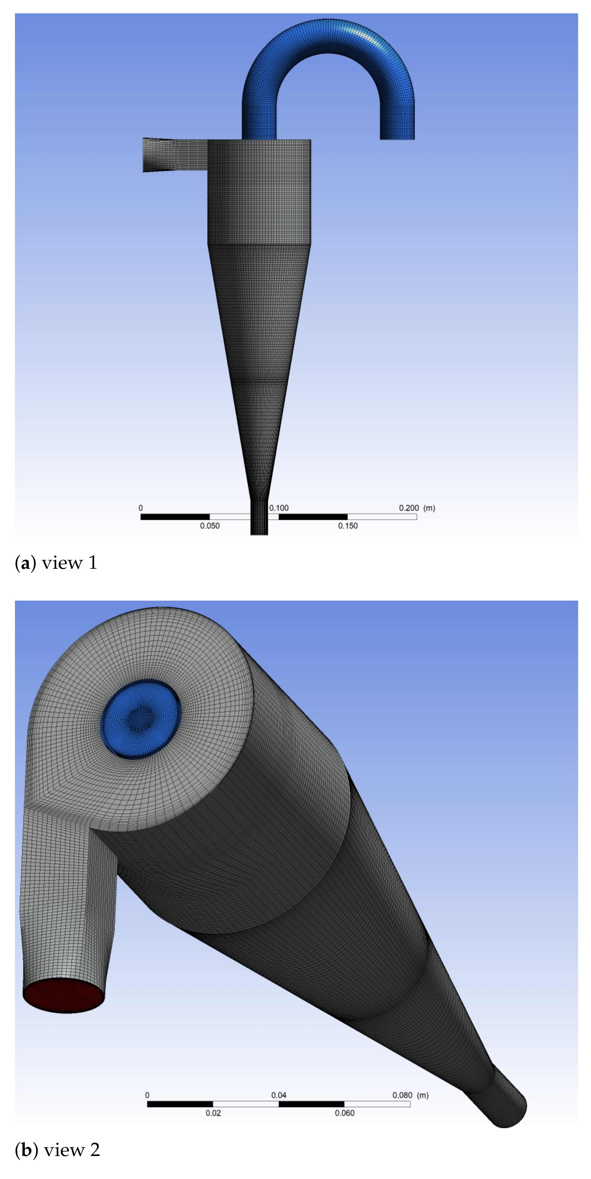
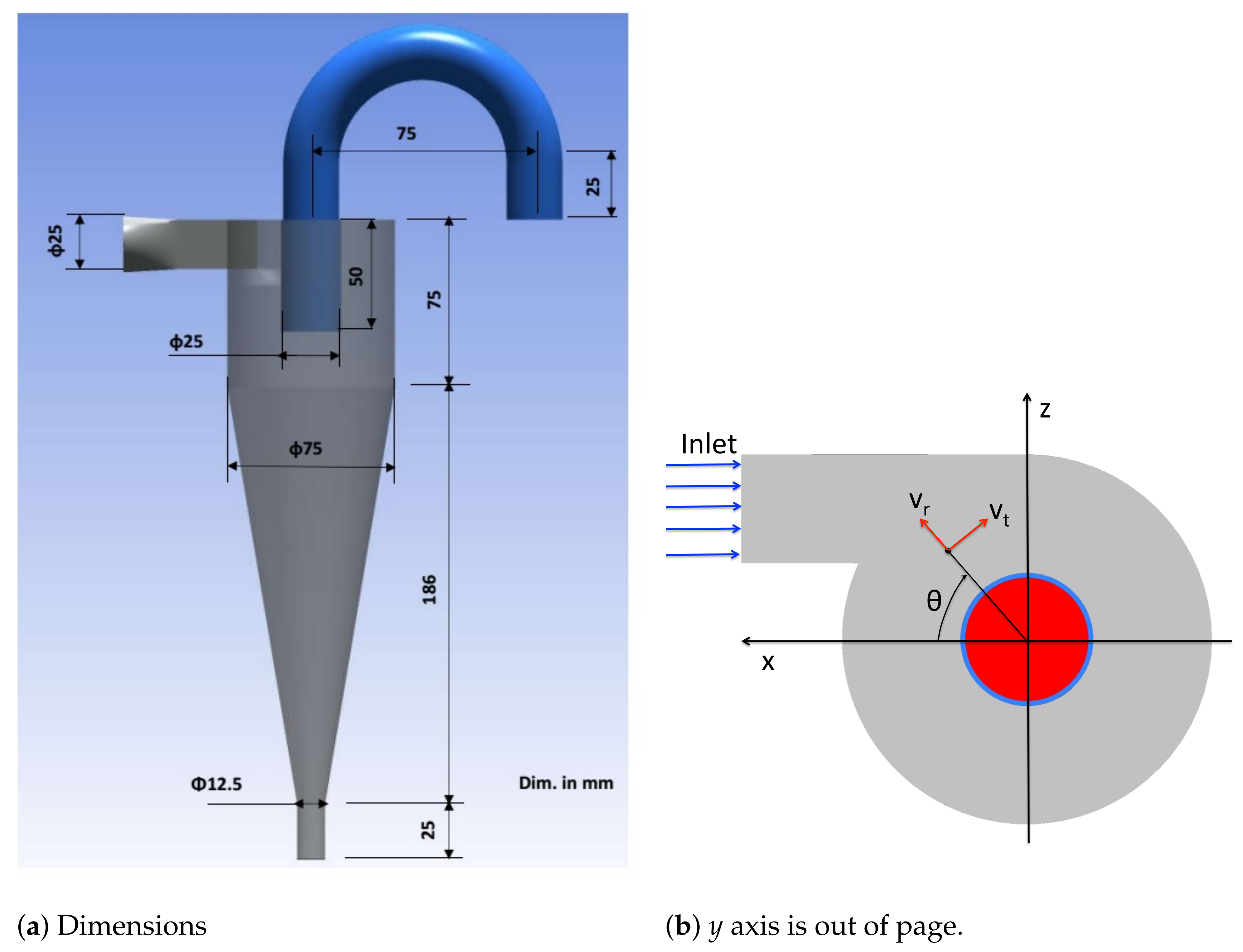
3. Computational Grid and Boundary Conditions

We used ICEMCFD software to construct the geometry of the hydrocyclone and generate Block-Structured O-type grid. The dimensions of the hydrocyclone are given by Hsieh [13] as shown in Figure 1a. The x and z axes of a right-handed coordinate system x y z are depicted in Figure 1b, the y axis is vertically upward and coincides with the hydrocyclone centerline. Axial locations are measured relative to the roof of the hydrocyclone such that a horizontal plane that is 60 mm below the roof is called y = 60 mm. Figure 1b also shows the definitions of the radial v r and tangential v t velocity components. The axial velocity v a is in the y direction. The inlet pipe is circular with diameter of 25 mm. We modified the cross-section of inlet pipe from circular at inlet to a square of equal area at the intersection with the cylindrical part. This modification of inlet pipe has been done to facilitate the construction of the block-structured mesh. The cylindrical part of hydrocyclone has inner diameter of 75 mm and its height equals 75 mm. The conical part of hydrocyclone extends vertically below the cylindrical part a distance of 186 mm. The diameter of this conical part decreases from 75 mm at intersection with cylindrical part and reaches 12.5 mm at intersection with spigot pipe. The cone angle is approximately 20 . The spigot pipe extends downward a distance of 25 mm. The overflow pipe (Vortex finder) has a diameter of 25 mm and extends a distance of 50 mm inside the cylindrical part of the hydrocyclone. This overflow pipe takes the shape of an elbow as shown in Figure 1a and maintains constant diameter. The exit boundary of the overflow pipe (on the right) is located at the same level of the roof of the hydrocyclone.
The interior of hydrocyclone is divided into 5 subdomains to generate appropriate grid-block in each subdomain and optimize the size of each hexagonal grid. As shown in Figure 2, the grid in the core of hydrocyclone and overflow pipe has been designed to resolve the high gradient of tangential and axial velocity components near the expected air core. We constructed five different grid sizes for the same set of blocks to study the effects of grid size on the quality of the results. Table 1 provides a summary of the grid sizes in our simulations. Resolving small scales vortical structures in the boundary layer requires a very fine mesh near the wall such that the first grid point off the wall is at y + 1 . To alleviate this stringent requirement, a near-wall model is employed, which is the default set up in ANSYS CFX. A wall function is used if the grid is too coarse to resolve the viscous sub-layer (say y + > 5 ). However, if the near-wall grid is fine ( y + < 2 ), the near-wall treatment provides a smooth transition from wall function modeling to grid-resolved viscous flow. For the three coarse meshes, where the surface average y + is around 18, the near-wall flow is modeled. For the fine mesh f2, the normal distance from the first grid point to the wall is 0.01 mm, and the surface average y + is 2.2. We expect the viscous sub-layer to be resolved for the fine mesh. The step sizes in the directions parallel to the wall are also estimated. In the axial direction, the step size in wall-units is 110, and in the circumferential direction it is 220. These are adequate mesh steps since the vortical structures in hydrocyclones are elongated in the circumferential direction.

Boundary Conditions and Numerical Method

The LES Euler–Euler model in CFX-ANSYS (V17.2) has been used to simulate the flow of air and water where the two phases are treated as interpenetrating continua. However, for the purpose of momentum exchange between the two phases, the water is declared as the continuous phase and air as dispersed phase. The boundary conditions are setup at inlet as velocity-inlet with a uniform value of 2.28 m/s that achieves mass flow rate of 1.117 kg/s of water. The water volume fraction at inlet is 1. The opening boundary condition has been selected for the exit boundaries of the overflow elbow and underflow pipe. The pressure at these boundaries has been specified as zero gauge pressure (i.e., atmospheric pressure) and the back flow has been selected to be 100 % air. No-slip condition with zero velocities is applied on hydrocyclone walls.
We use bounded central difference to discretize the continuity and momentum equations of air and water phases. The bounded central-difference schemes are second-order accurate and can damp dispersive errors in central-difference schemes. A second-order implicit Euler method is used for time integration. The value of time step is important to stabilize calculations of LES models. Most of the results presented here are obtained for a time step Δ t = 10 4 s. Some of the results as indicated are obtained with a smaller time step Δ t = 5 × 10 5 s. The residence time in Hsieh’s hydrocyclone is about 1 second. The first simulation uses coarse grid c1 (2.4 million elements) and is initialized with 100% water. It is executed for at least 3 s until the air core is established and the flow reached statistically steady state. The flow on this grid is then interpolated to initialize simulations on other grids c2, c3 and f1. Converged solution on f1 is interpolated to initialize solution on the finest grid f2. The simulation on each grid after interpolation is continued for at least one second before mean flow and turbulence statistics are computed over an additional one second.

4. Results: Two-Fluid Model

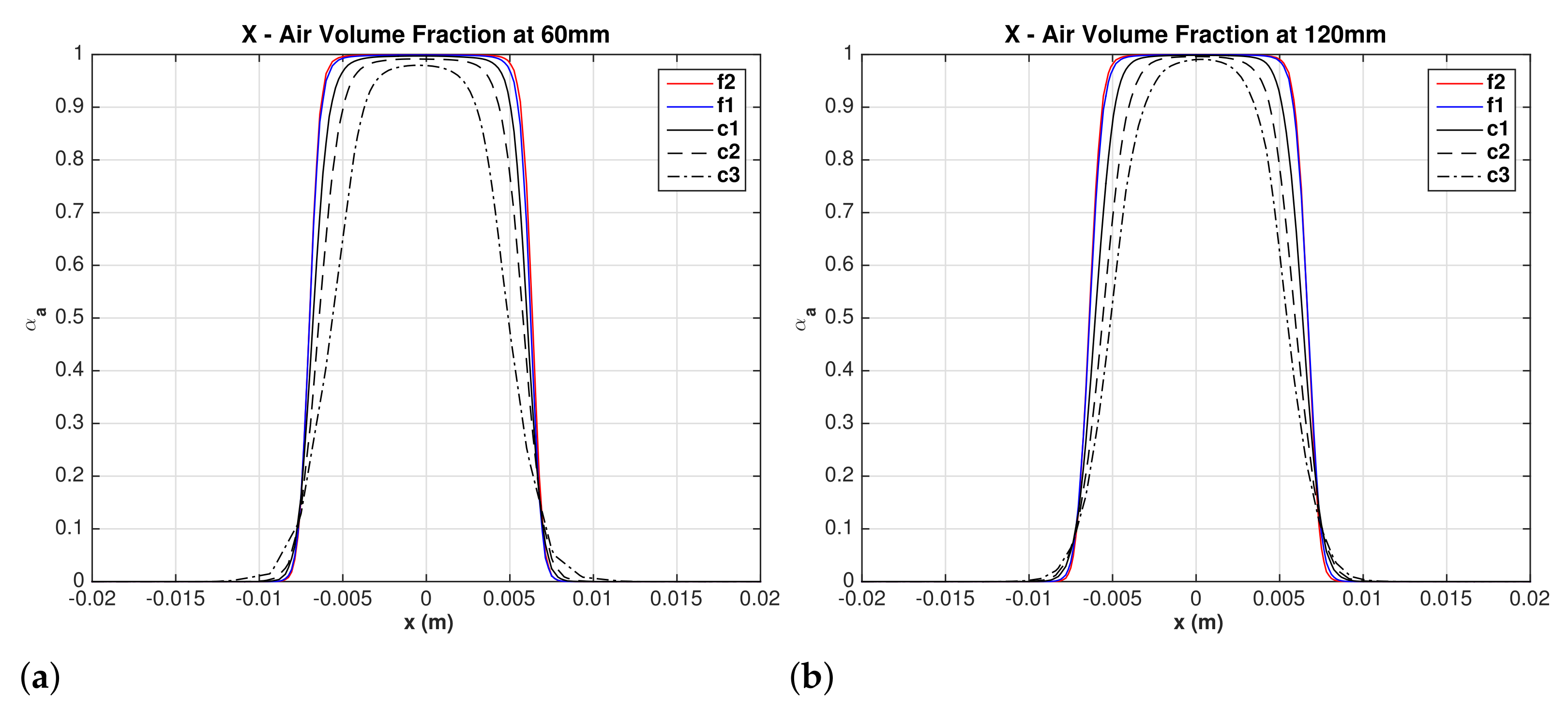
4.1. Inlet Pressure, Split Ratio, and Air Core

The water volume flow rate at the inlet is prescribed and is steady in time. However, the inlet pressure and water volume flow rates to the overflow and underflow are predicted in the course of simulations and they fluctuate in time. Their time-averaged values are given in Table 1. %Overflow is the water volume flow rate exiting from the top opening as a percentage of water volume flow rate at the inlet of hydrocyclone. Different mesh resolutions show good comparison with experimental data by Hsieh [13] for these overall measures of the hydrocyclone performance. Although the coarsest mesh shows lower percentage errors than finer meshes, the mean velocity profiles and turbulence statistics for such a coarse mesh are much less accurate.
Air is drawn from the underflow opening as a result of the low pressure on the axis of hydrocyclone. The air core is nearly a cylindrical surface that extends axially from the underflow opening to the overflow exit. The instantaneous air-core surface fluctuates radially and twists by its interaction with the upward flowing swirling turbulent water flow. The time-averaged of air volume fraction is used as an indicator of the air core. Figure 3a,b) show mean air volume fraction profiles on a horizontal line at 60 and 120 mm from the roof of hydrocyclone. For the finest mesh f 2 , the air volume fraction is nearly 1 over a diameter of 10 mm and drops to 0 beyond a diameter of 15 mm. Hsieh [13] reported an air-core diameter of 10 mm. Because of the fluctuating position of the air-water interface in addition to numerical diffusion, a sharp interface is difficult to predict. The figures show that as the mesh is refined the thickness of air-water mixture decreases, it is the largest for the coarsest mesh c 3 , but the profiles are nearly identical for the fine meshes f 1 and f 2 .

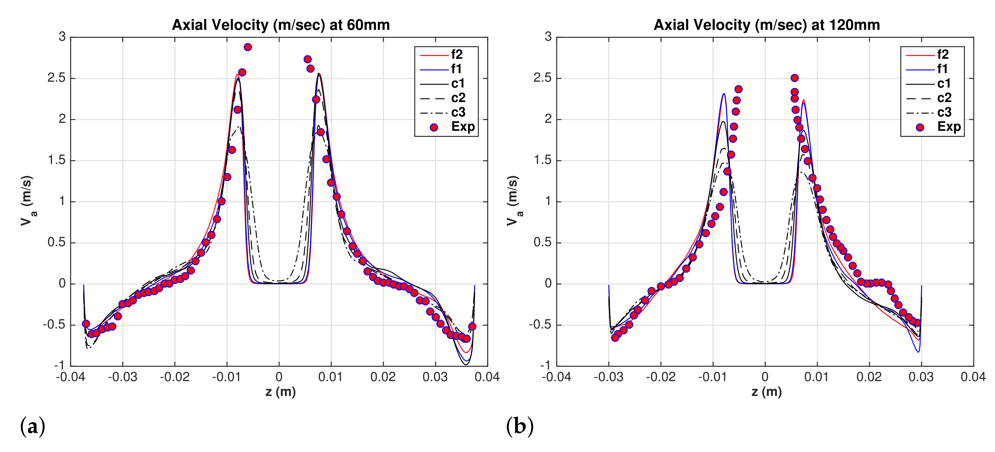
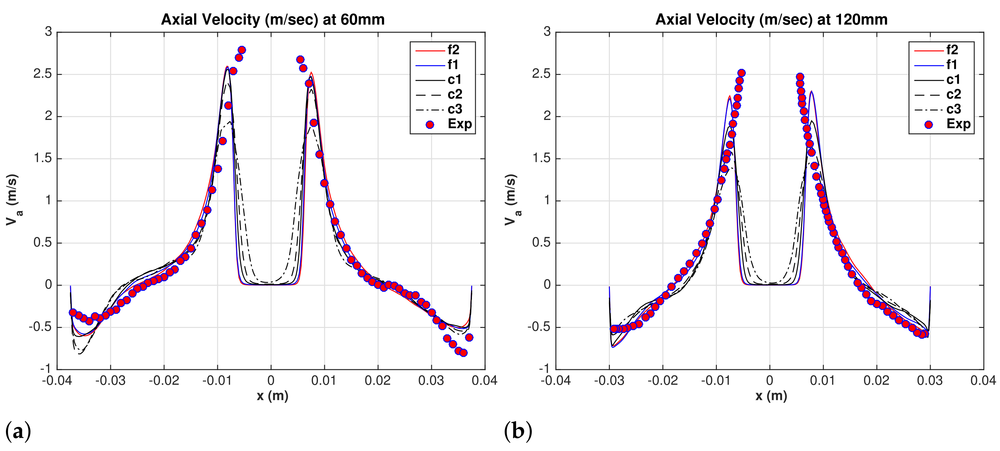
4.2. Mean Water Superficial Axial Velocity

The axial flow in a hydrocyclone has a complex structure. The near-wall flow is downward, and it appears as a swirling wall jet, while on the inside the flow is a swirling upward flow bounded by a free surface (air core). Comparisons between experimental data by Hsieh [13] [(0, 180 ) data] and LES results for the mean superficial water axial velocity are shown in Figure 4a,b at y = 60 and y = 120 mm, respectively. The maximum upward axial velocity increases as the grid is refined, and convergence is established for the fine meshes f 2 and f 1 where the profiles are almost identical near the air core. The experimental data indicates a smaller core diameter with maximum axial velocity inward. The data also show a plateau in the axial velocity at y = 120 mm which cannot be predicted by grid refinements. Further comparisons with experimental data [Hsieh [13] (90 , 270 ) data] are shown in Figure 5a,b. The overall agreement between LES and experimental data is fair.

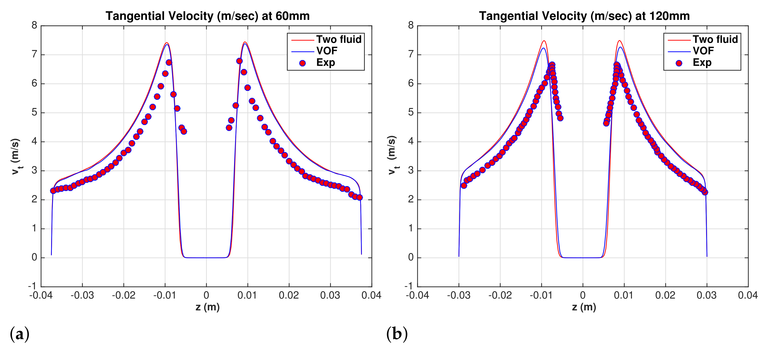
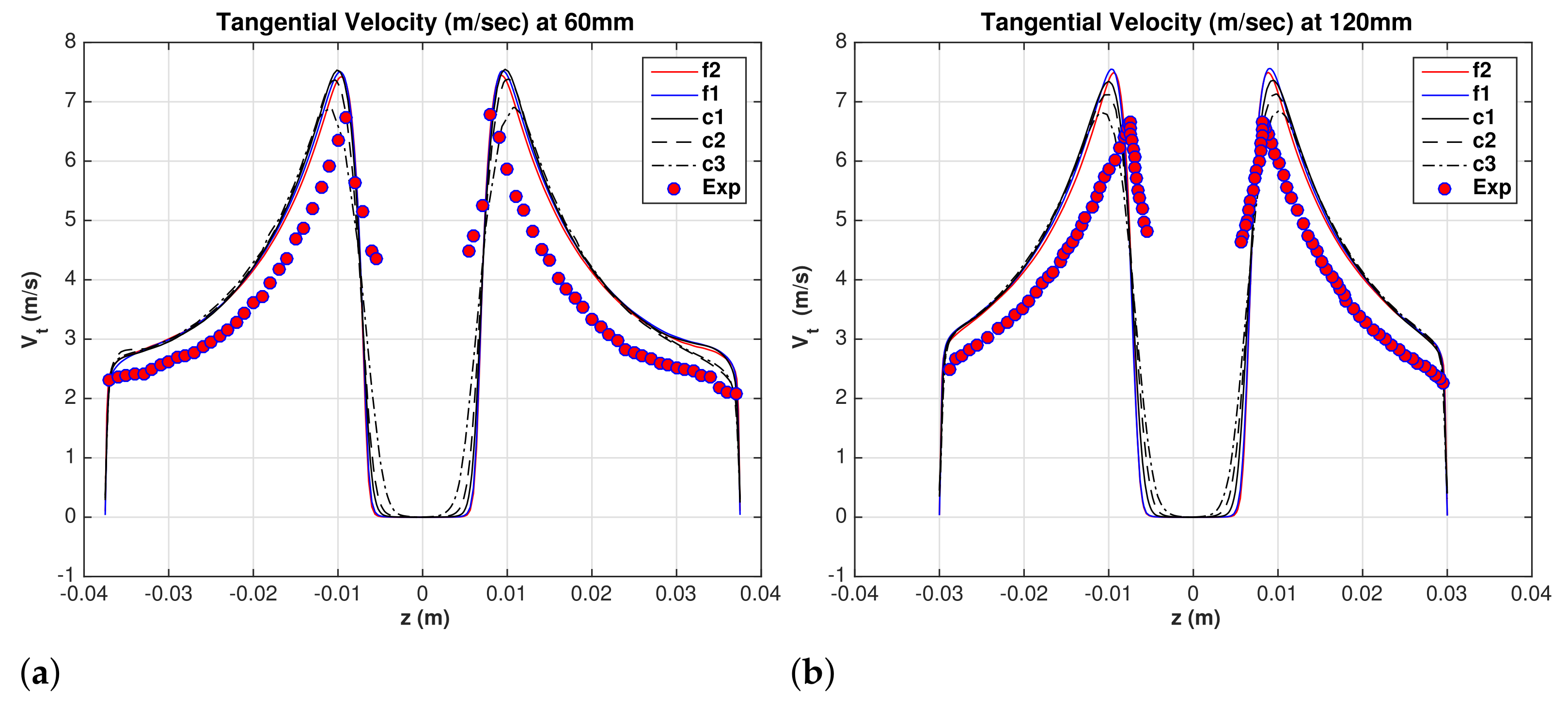
4.3. Mean Water Superficial Tangential Velocity

Comparisons between experimental data [Hsieh [13] (0, 180 ) data] and LES results for the mean superficial water tangential velocity are shown in Figure 6a,b at y = 60 and y = 120 mm, respectively. The maximum tangential velocity increases with grid refinement, but it is consistently higher than the experimental data. It is a coincidence that the maximum tangential velocity of the coarsest grid c3 agrees with the experimental data, and as a results the predicted inlet pressure shown in Table 1 is also in agreement with the measured pressure. Except for the coarsest grid c3, the tangential velocity profile is less sensitive to grid resolution. All grids approach the same profile. The persistent difference between the experimental data and LES cannot be attributed to grid effects. No attempt is made here to adjust the exit pressures or other operating conditions to reduce that shift in the tangential velocity. The effects of the turbulence model on the tangential velocity profile is presented in Section 6.

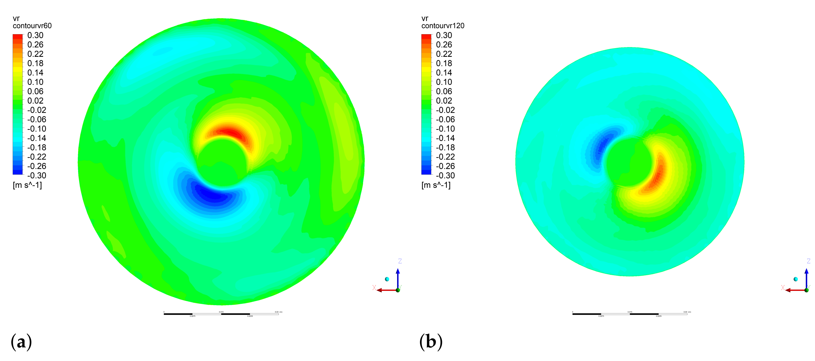
4.4. Mean Water Superficial Radial Velocity

In hydrocyclones, the radial velocity is of a much smaller magnitude than the axial and tangential components, but it may have important effects on particles transport. The present simulations show a complex distribution of the radial velocity component. Figure 7a,b show mean water superficial velocity contours in planes y = 60 and 120 mm, respectively. The maximum magnitude is less than 0.4 m/s. On a diagonal, the velocity is radially outward (positive) on one side of the air core, and radially inward (negative) on the opposite side of the air core. Such a distribution also rotates with the swirling flow. Isosurfaces of mean water superficial radial velocity, v r = ± 0.2 m/s are shown in Figure 8a, the spiral structure causes bending of the air core as shown in Figure 8b which shows velocity vectors colored by the radial velocity in the x y plane. These figures also show a streamwise vortex initiated at the inlet to the cylindrical part of hydrocyclone.

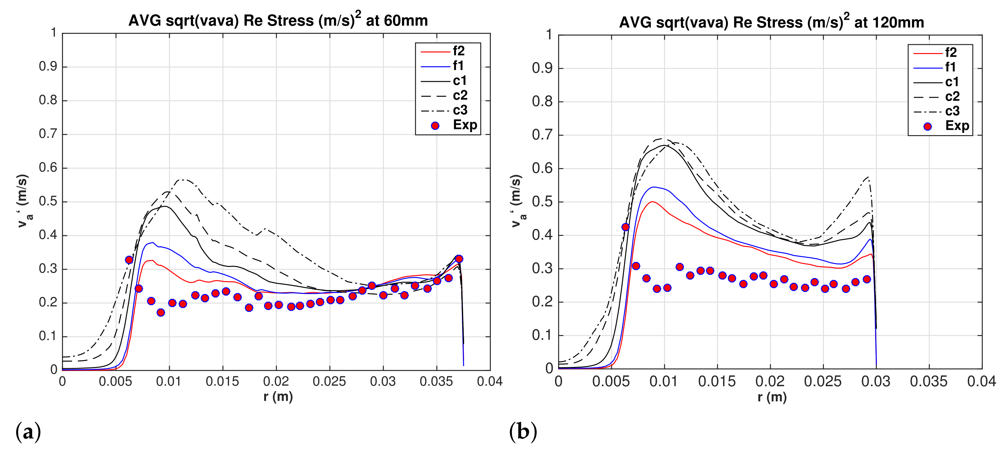
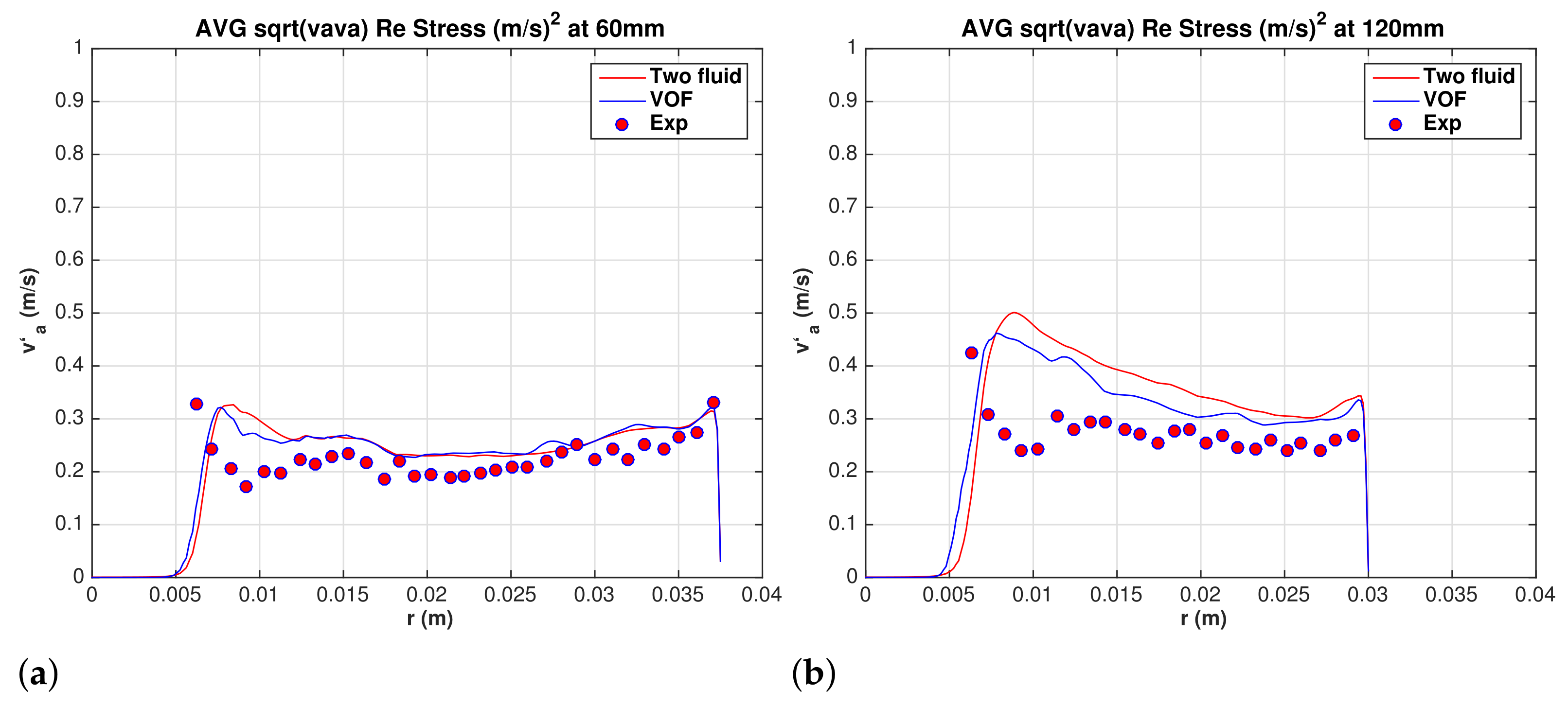
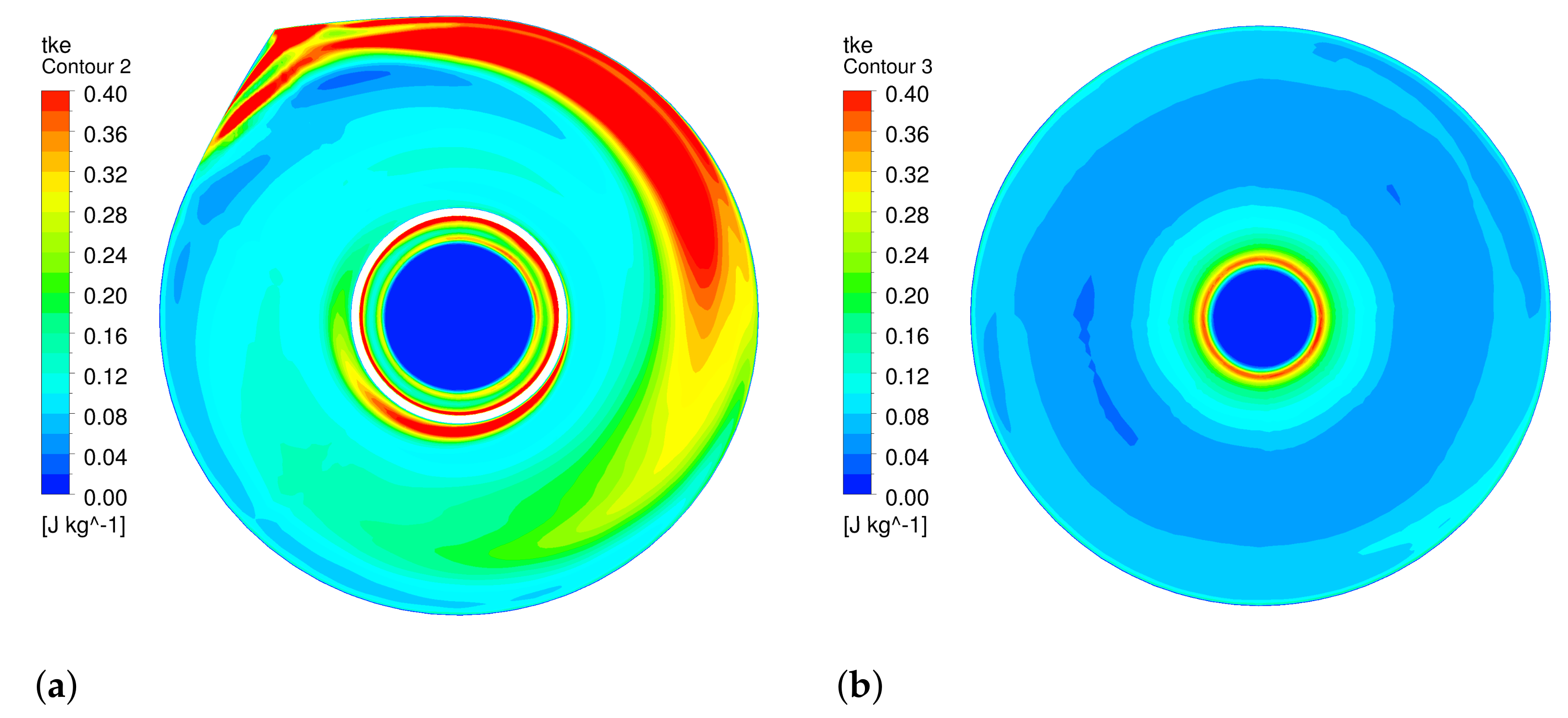
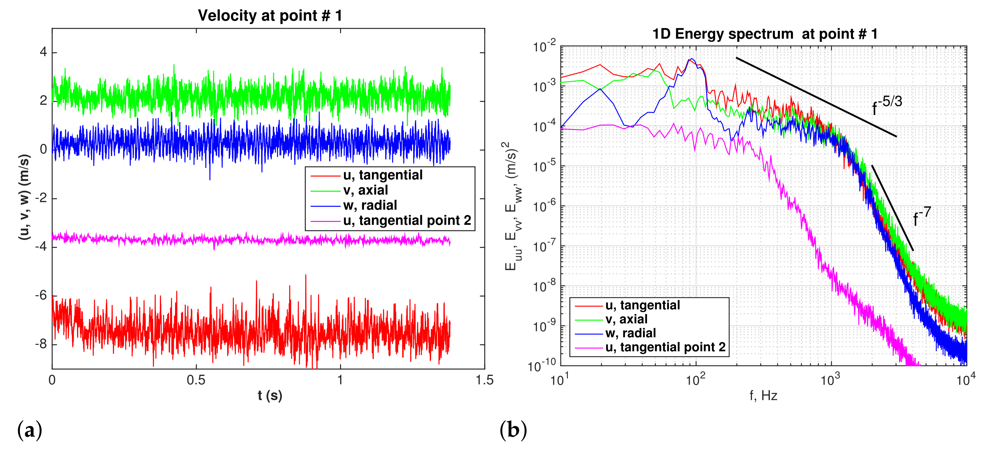
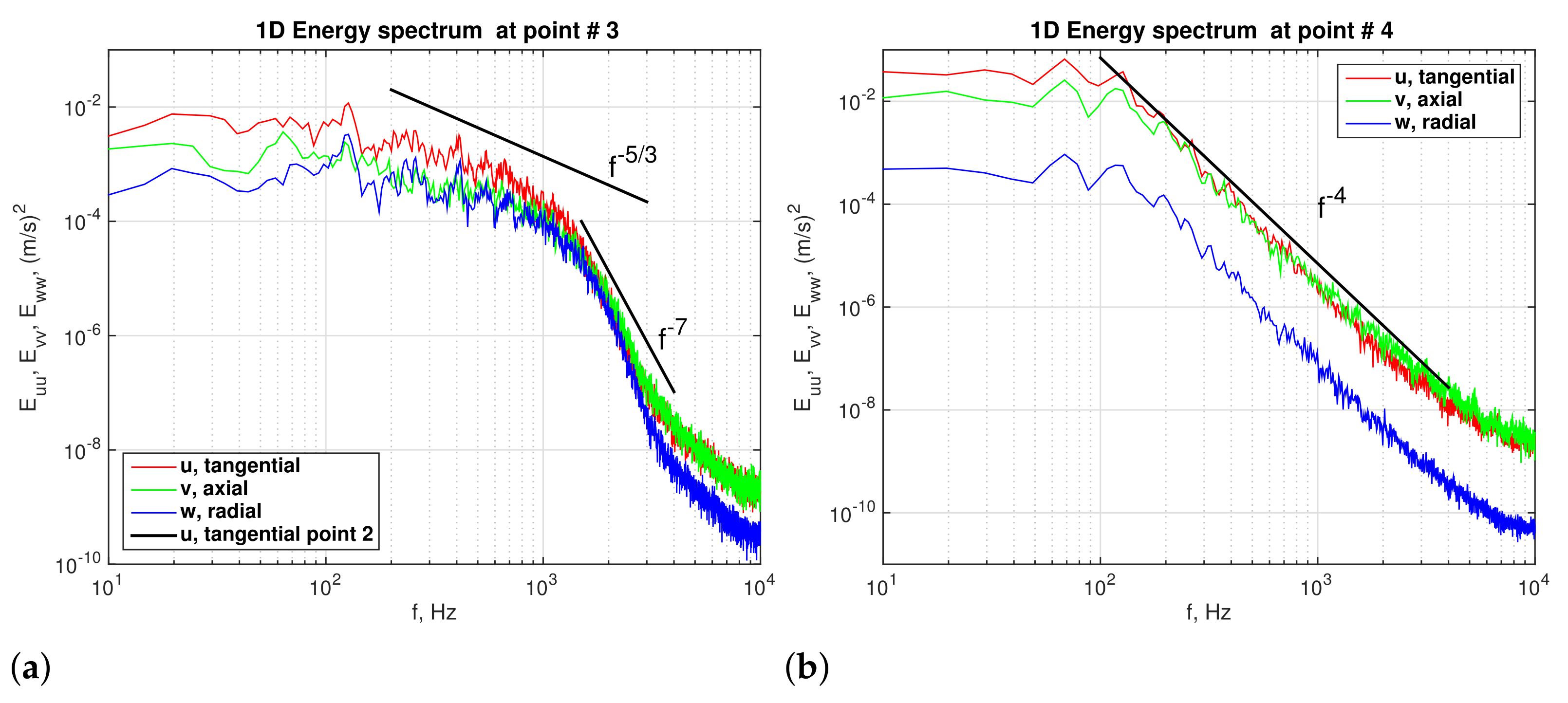
4.5. Resolved Normal Reynolds Stresses and Energy Spectra

Investigation of the radial distribution of circulation on circles centered on the axis shows that the circulation increases with radius except in a very thin layer near the solid wall where the circulation drops to zero. Such a distribution is centrifugally stable [31]. Sreedhar and Ragab [32] conducted LES for an Oseen vortex whose circulation increases with radius and showed that initial random disturbances are damped by the centrifugal field. Thus, the swirl in the boundary-layer flow and the shear of the axial flow must be sources of turbulence production in a hydrocyclone. After the flow reached statistically steady state, time-averaging over at least one second is performed for computing turbulence statistics such as Reynolds stresses and turbulent kinetic energy. Normal Reynolds stresses of the resolved large-scale turbulence are presented as the root-mean-square (RMS) of the water superficial velocity fluctuations. Hsieh’s [13] experimental data are provided on a radial line. For the sake of comparison, LES data are averaged on four radial lines along the x and z axes. Figure 9a,b show the axial component v a at elevations y = 60 and 120 mm, respectively. The LES data show consistent convergence to the experimental data with mesh refinement. The two fine meshes f 1 and f 2 are in satisfactory agreement with experimental data, but the coarser meshes over-predict the axial fluctuations. A fine mesh in the axial direction is necessary to capture the axial turbulence length scales. In the cylindrical region of hydrocyclone at y = 60 mm, the near-wall region is well predicted by all grids, but the significant difference happens near the air core. In the conical region at y = 120 mm, the finest mesh f 1 shows the best agreement with experimental data; however, further refinement might be of little effects.
Figure 10a,b show the tangential component v t at elevations y = 60 and 120 mm, respectively. LES data for meshes f 1 and f 2 are in very good agreement with Hsieh’s [13] data. The results for the coarse mesh c 1 are also in fair agreement with experimental data. The tangential fluctuations show less sensitivity to grid resolution than the axial fluctuations. It will be shown later that the turbulent eddies are elongated in the circumferential direction relative to the axial and radial directions which requires much finer mesh size in these directions than the circumferential direction.
Figure 11a,b show LES data for the radial component v r at elevations y = 60 and 120 mm, respectively, but no experimental data are available in Hsieh [13]. Convergence with mesh refinement is clearly demonstrated for the RMS of radial velocity fluctuations. The radial fluctuations are comparable to the axial fluctuations but they become stronger in the conical section. In fact, all the three normal Reynolds stress components or velocity fluctuations RMS increase in the conical section of the hydrocyclone.
Turbulent kinetic energy of resolved scales in a vertical plane ( x = 0 ), which is normal to the inlet stream, are shown in Figure 12a. High turbulent kinetic energy is generated just below the volute and continues in the cylindrical section. Contours in a horizontal plane y = 24 mm, which is very close to the bottom of inlet volute, depicted in Figure 13a show the high levels of turbulent kinetic energy generated as the flow enters the hydrocyclone. However, as turbulence becomes subjected to the stabilizing swirling flow, turbulent kinetic energy is reduced at the end of the cylindrical section and beginning of the conical section as shown by the annular region of low turbulent kinetic energy in Figure 12a. The reduced turbulent kinetic energy is also shown in Figure 13b by contours in a horizontal plane y = 82 mm below the roof of hydrocyclone. Localized regions of low turbulent kinetic energy can be seen also in Cui et al. [33]; however, their locations are affected by the vortex finder diameter.
Fluctuations of the velocity components are monitored at four points labeled points 1 to 4 with coordinates ( x , y , z ) = ( 0 , 60 , 8 ) , (0,76,23), (0,186,8), (0,203.8,15.73) mm, where y is measured from the roof, see Figure 12a. Points 1 and 3 are near the air-water interface, point 2 falls near the center of low turbulent kinetic energy region, and point 4 is near the wall in the lower conical section. Time history of velocity components at point 1 is shown in Figure 14a and the corresponding turbulent energy spectra (computed using the Welch method [34]) are shown in Figure 14b. The spectra for the tangential and radial velocity components show a peak at a frequency of approximately 100 Hz. Such a peak is absent in the spectrum of the axial velocity. Thus, the air core is subjected to larger fluctuations in horizontal planes. The stabilizing effect of the swirling flow is further demonstrated by comparing the tangential velocity fluctuations at points 1 and 2 as shown in Figure 14a and their energy spectra shown in Figure 14b. The flow is almost locally re-laminarized in the low turbulent kinetic annular region. Using LES, Ragab and Sreedhar [35] found that a centrifugally stable vortex flow can quench the large-scale turbulent structures generated by instabilities of an axial velocity with inflection point and renders the flow to a laminar state. Except near the wall, the mean tangential velocity profile in the current hydrocyclone is centrifugally stable. In the conical region, the turbulent kinetic energy is maximum near the air-water interface and near the wall. The energy spectra at two points in the high kinetic energy regions are shown in Figure 15a for point 3 and in Figure 15b for point 4. An inertial subrange with slope of −5/3 is clearly evident for the point near the air core, where the tangential velocity fluctuations are dominant. The spectra for the point near the wall do not show an inertial subrange instead turbulent energy of small scales decays as f 4 . The kinetic energy is contained in the fluctuations in the tangential and axial velocity components, and energy of the radial component is an order of magnitude smaller.
To visualize turbulent large-scale structures in the hydrocyclone, we define the instantaneous fluctuating component of tangential vorticity ω θ
ω θ = ω θ < ω θ >
Isosurfaces of ω θ = ± 500 s 1 are depicted in Figure 12b, the high values near the walls are filtered for clarity of the interior region. The length scales in the axial and radial directions are much smaller than the circumferential length scale. In the annular region of low turbulent kinetic energy those high levels of vorticity are suppressed, but they persist around the air core. The generation of such vortical structures must be attributed to the shear associated with complex form of the axial velocity profile.

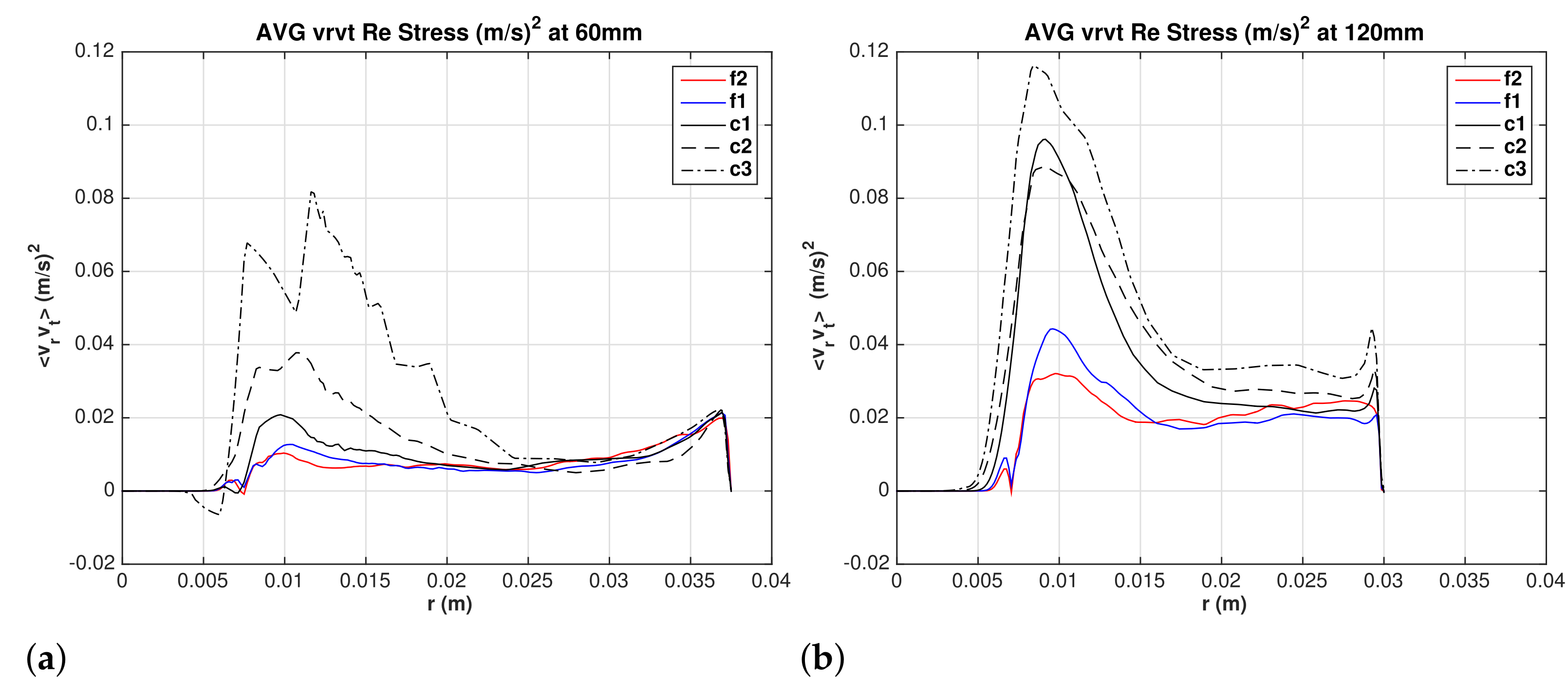
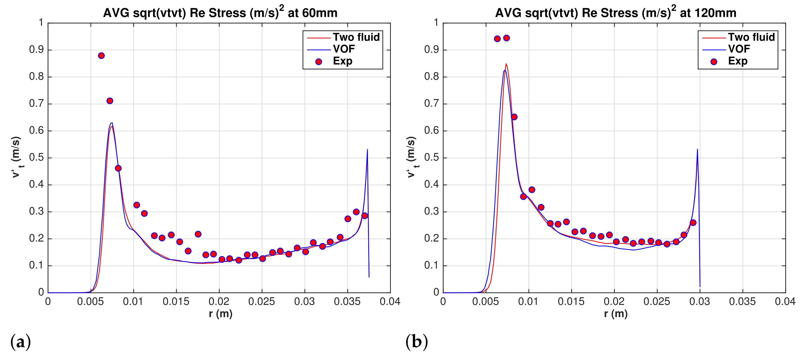
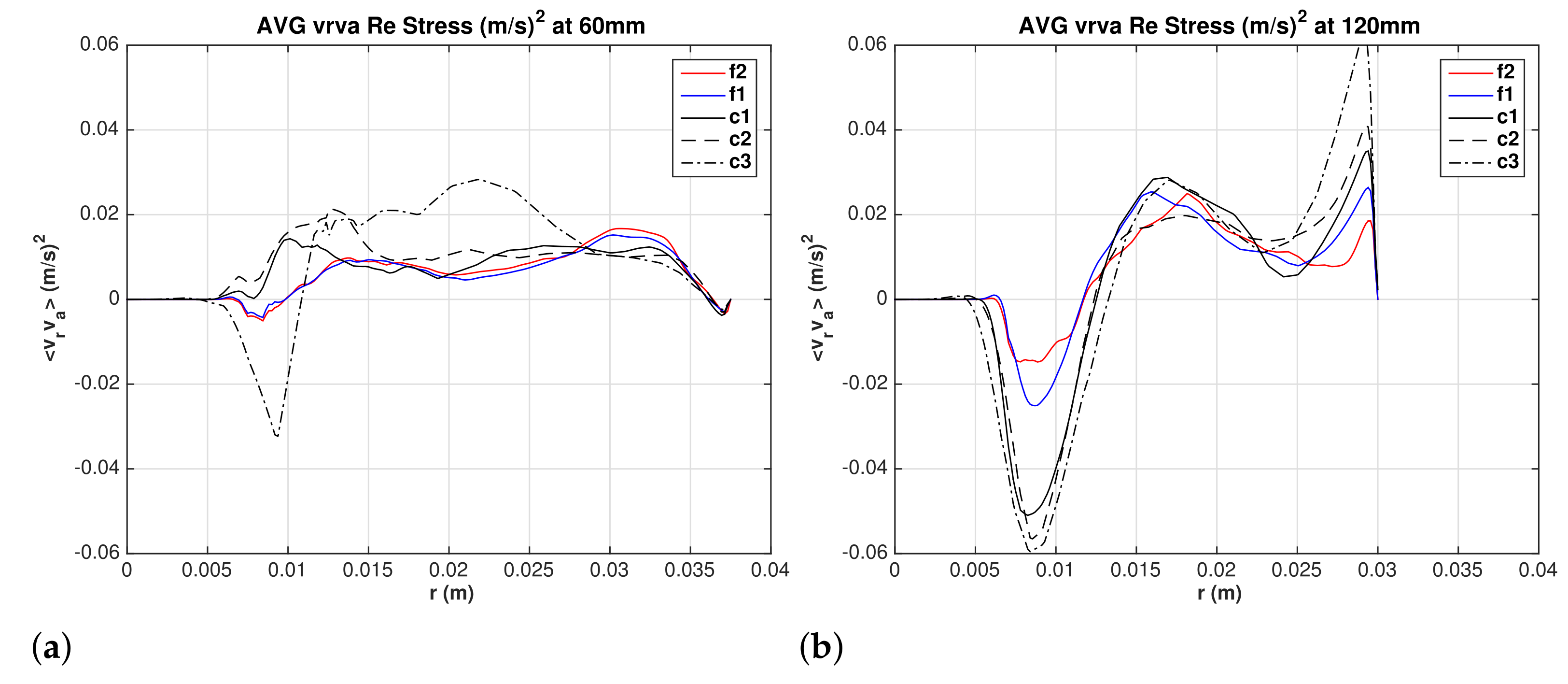
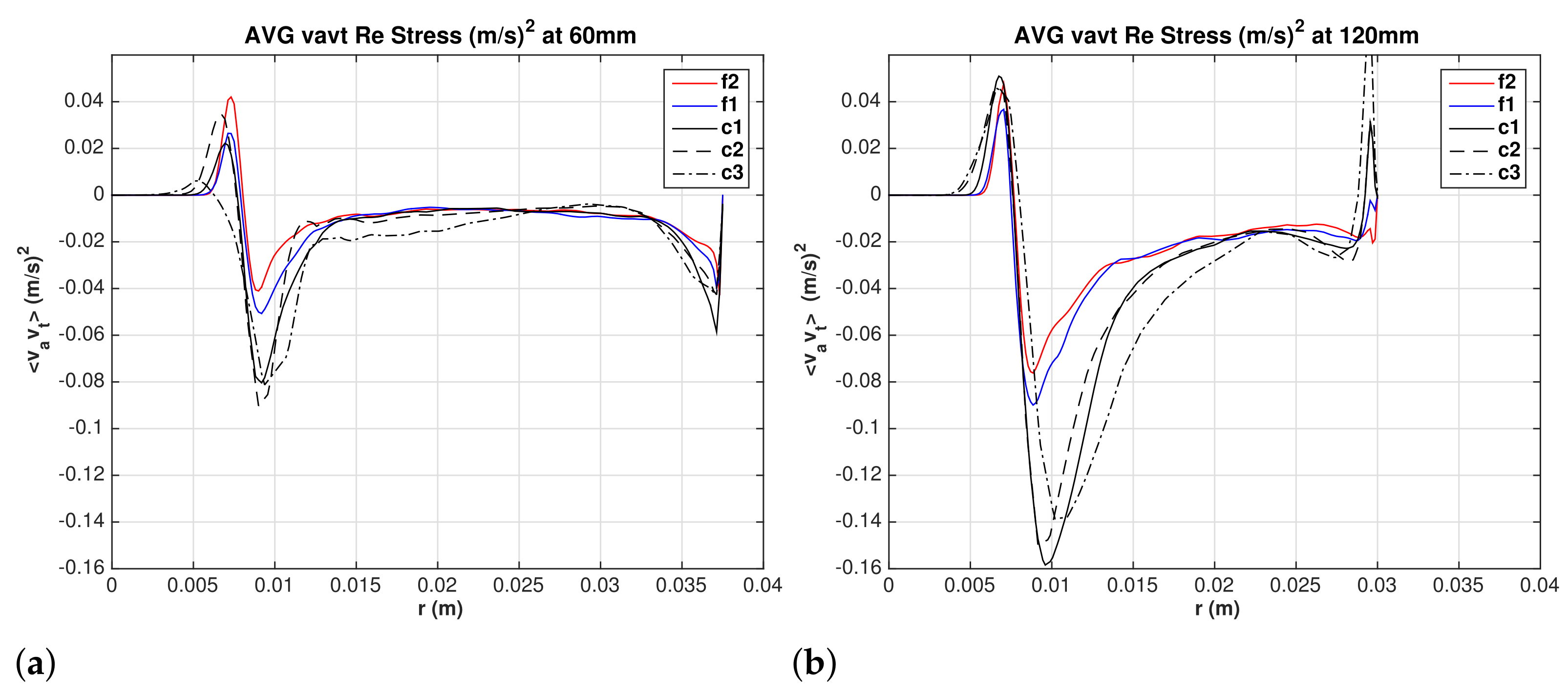
4.6. Resolved Shear Reynolds Stresses

The three components of resolved shear Reynolds stresses in cylindrical coordinates ( < v r v a > , < v r v t > , < v a v t > ) are shown in Figure 16, Figure 17 and Figure 18 at the two elevations y = 60 and 120 mm. Results for different grids demonstrate the importance of mesh refinement for capturing these Reynolds stresses. Satisfactory grid convergence is established for the fine meshes f 1 and f 2 . No experimental data are available for validation. The near-wall and the air-core regions are regions of intense shear stresses. All three components acquire stronger magnitudes as the flow go down the conical section.

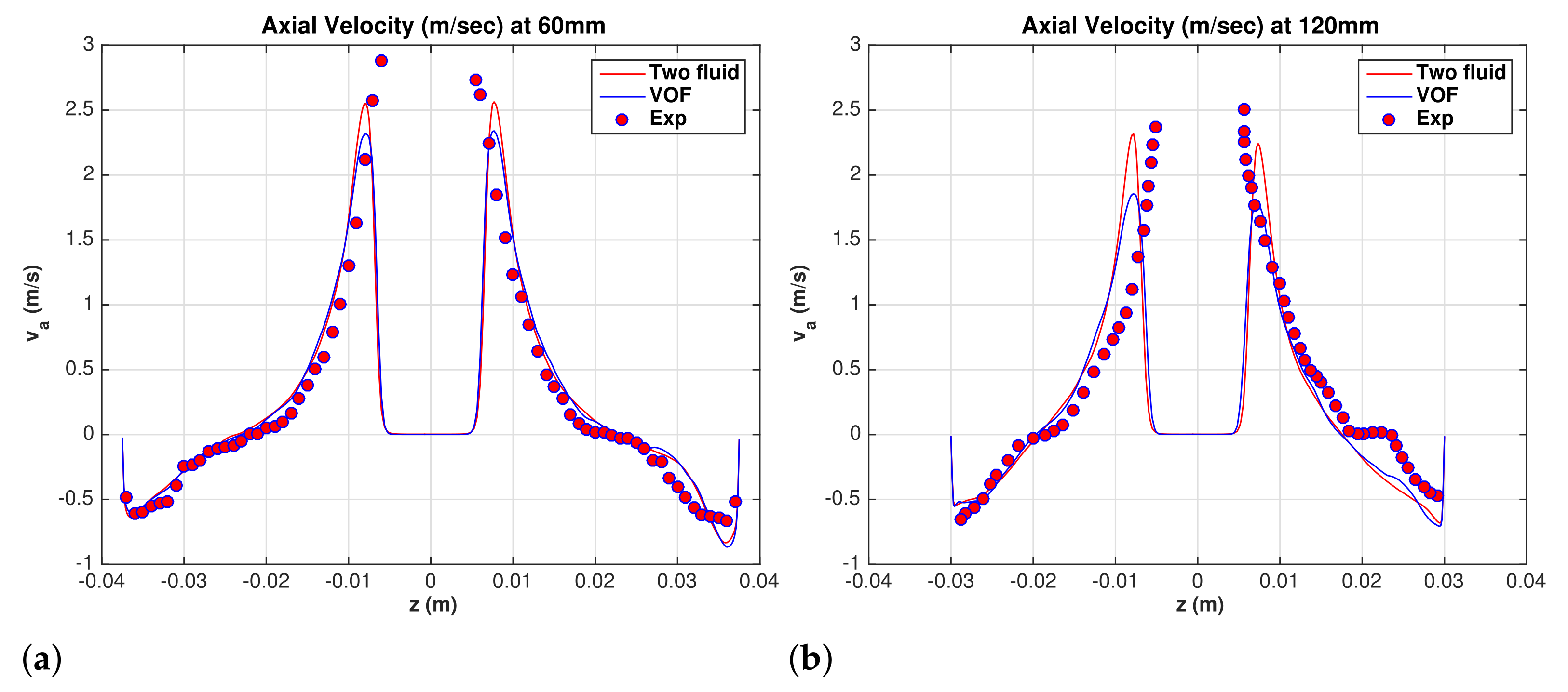
5. Comparison of Volume-of-Fluid and Two-Fluid Models

It is important to validate the two-fluid (Euler–Euler) model used in the present paper by comparing the results with VOF model, the later model is commonly used to resolve air core–water interface in hydrocyclones of the present type. However, the two-fluid model is the natural choice for air-sparged hydrocyclones where there are a huge number of bubbles and resolving the gas-liquid interfaces is not computationally feasible by VOF, [26]. The finest mesh f2 is used for both models. Comparisons of mean water superficial velocity profiles are shown in Figure 19a,b for the axial velocity and in Figure 20a,b for the tangential velocity. Velocity profiles predicted by the two models are in good agreement. The maximum axial velocity near the air-water interface is somewhat lower in VOF model than in the two-fluid model. The persistent difference between experimental data and simulation in the tangential velocity could not be reduced by the VOF model. Large-eddy simulations by Durango et al. [36] also show the shift in tangential velocity.
Axial and tangential turbulence velocity fluctuations (RMS) profiles are also compared in Figure 21a,b and Figure 22a,b, respectively. The VOF results show lower axial velocity fluctuations in the conical section at section y = 120 mm from the hydrocyclone top. Overall, excellent agreement between the two models is observed.

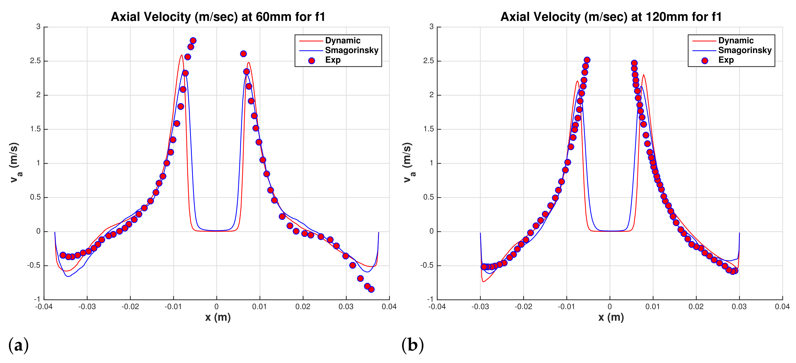
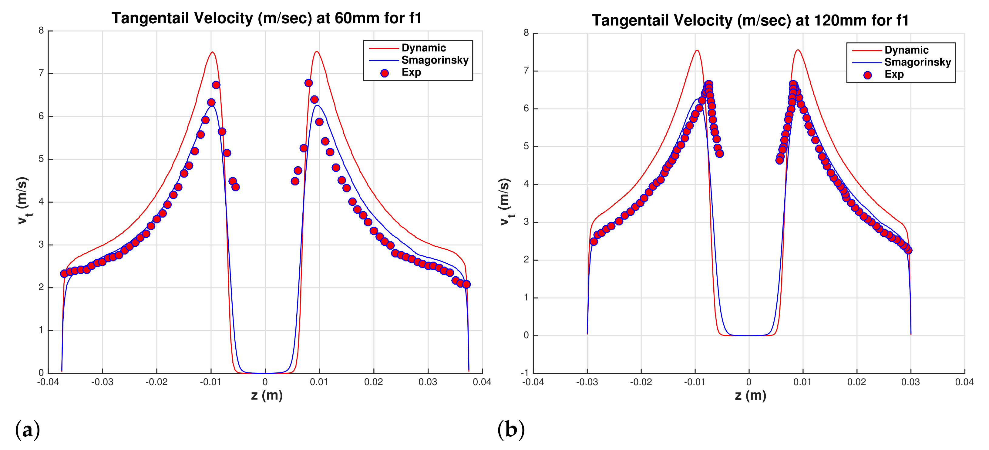
6. Effects of Subgrid-Scale Turbulence Model

It is unsettling to see the persistent shift in the mean tangential velocity between experimental data and LES results. This shift is predicted on all five meshes and for the VOF and two-fluid models. In the present study, an eddy viscosity is used, and the dynamic model is used to compute the model coefficient. The dynamic subgrid stress turbulence model is deemed more adequate than Smagorinsky model for turbulent flows that may be subjected to re-laminarizing mechanisms. Using Smagorinsky model with model constant C s = 0.12 , simulations are repeated for the two-fluid model on fine grid f1. Figure 23a,b show comparison between the dynamic model and Smagorinsky model results for the mean axial velocity. The two models are in good agreement. The results for the mean tangential profiles are shown in Figure 24a,b. Mean tangential velocity profiles predicted by Smagorinsky model, with adjusted model coefficient of 0.12, are in good agreement with the experimental data. However, the maximum velocity is under-predicted and hence the pressure drop between inlet and outlet is also under-predicted. Simulations using a smaller value for the model coefficient brought tangential velocity profiles of Smagorinsky model closer to the dynamic model profiles. Feiz et ai. [37] conducted LES for turbulent flow in a rotating pipe and compared their results with direct numerical simulations by Orlandi and Fatica [38]. They concluded that the dynamic model is more accurate than Smagorinsky model. The centrifugal field in the rotating pipe problem can have stabilizing effects as the swirling flow of the hydrocyclone.

7. Conclusions

Turbulent two-phase flow in a classifying hydrocyclone has been investigated using LES. The two-phase aspect of the flow is modeled by the two-fluid (Euler–Euler) and volume-of-fluid (VOF) models. Mean velocity and turbulence statistics show good comparison between the two-phase models. Thus, the present study validates the two-fluid model against the commonly used VOF for this type of hydrocyclone. The two-fluid model can be used for simulations of classifying as well as air-sparged hydrocyclones for which VOF is impracticable. The present study encourages application of the multi-fluid model to three-phase flow (liquid, solid particles, gas) in hydrocyclones.
Simulations on fine meshes 5.86 and 7.4 million elements enable capturing helical vortices as the dominant large-scale turbulent structures in the hydrocyclone. The turbulence structure in hydrocyclones is complex because of the competing effects of a stabilizing swirling flow and turbulence producing shear associated with the axial flow. Except near the wall, the free-vortex tangential velocity decays slower than the inverse of the radial distance measured from the axis. Such a distribution is centrifugally stable, and it can quench turbulence generated by other instabilities in the flow. Significant reduction in the turbulent kinetic energy is predicted at the end of the cylindrical section and beginning of the conical section. The flow is nearly re-laminarized in an annular region at the beginning of the conical section. High turbulent kinetic energy prevails near the air-water interface. The energy spectra at points near the interface show a short inertial subrange where energy decays as f 5 / 3 , followed by damping where energy drops as f 7 , where f is frequency. For points in the boundary layer where high turbulent kinetic energy is found, the energy spectra exhibit f 4 decay.
Mean velocity profiles and normal Reynolds stresses are in fair agreement with experimental data by Hsieh [13]. However, LES results with the dynamic subgrid model over-predict the experimental data for tangential mean velocity. Using Smagorinsky model, one may obtain better agreement with the experimental data by adjusting the model constant. However, such an approach is not adequate for turbulent flows that involve regions of intense turbulence that are subjected to stabilizing or re-laminarizing mechanism as is the case of hydrocyclones.

Author Contributions

Conceptualization, H.F and M.B.; methodology, S.R.; software, H.F.; data curation, M.B. and S.R.; writing—original draft preparation, S.R.; writing—review and editing, H.F. and M.B.; All authors have read and agreed to the published version of the manuscript.

Funding

This research received no external funding.

Conflicts of Interest

The authors declare no conflict of interest.

References

  1. Restarick, C.J. Adjustable Onstream Classification Using A Two Stage Cylinder-Cyclone. Miner. Eng. 1991, 4, 279–288. [Google Scholar] [CrossRef]
  2. Nowakowski, A.; Cullivan, J.; Williams, R.A.; Dyakowski, T. Application of CFD to modelling of the flow in hydrocyclones. Is this a realizable option or still a research challenge? Miner. Eng. 2004, 17, 661–669. [Google Scholar] [CrossRef]
  3. Rovinsky, L.A. Application of separation theory to hydrocyclone design. J. Food Eng. 1995, 26, 131–146. [Google Scholar] [CrossRef]
  4. Narasimha, M.; Mainza, A.; Holtham, P.; Brennan, M. Air-core modelling for hydrocyclones operating with solids. Int. J. Miner. Process. 2012, 102, 19–24. [Google Scholar] [CrossRef]
  5. Hararah, M.A.; Endres, E.; Dueck, J.; Minkov, L.; Neesse, T. Flow Conditions in The Air Core of The Hydrocyclone. Miner. Eng. 2010, 23, 295–300. [Google Scholar] [CrossRef]
  6. Devulapalli, B. Hydrodynamic Modeling of Solid-Liquid Flows in Large-Scale Hydrocyclones; The University of Utah: Salt Lake City, UT, USA, 1996. [Google Scholar]
  7. Slack, M.; Del Porte, S.; Engelman, M. Designing automated computational fluid dynamics modelling tools for hydrocyclone design. Miner. Eng. 2004, 17, 705–711. [Google Scholar] [CrossRef]
  8. Ghodrat, M. Computational Modelling and Analysis of the Flow and Performance in Hydrocyclones. Ph.D. Thesis, School of Materials Science and Engineering, The University of New South Wales, Kensington, Australia, 2014. [Google Scholar]
  9. Manninen, M.; Taivassalo, V.; Kallio, S. On the Mixture Model for Multiphase Flow. 1996. Available online: https://www.osti.gov/etdeweb/biblio/434874 (accessed on 24 August 2021).
  10. Cullivan, J.; Williams, R.A.; Cross, R. Understanding the hydrocyclone separator through computational fluid dynamics. Chem. Eng. Res. Des. 2003, 81, 455–466. [Google Scholar] [CrossRef]
  11. Narasimha, M.; Sripriya, R.; Banerjee, P. CFD modelling of hydrocyclone—Prediction of cut size. Int. J. Miner. Process. 2005, 75, 53–68. [Google Scholar] [CrossRef]
  12. Narasimha, M.; Brennan, M.; Holtham, P. Large eddy simulation of hydrocyclone—Prediction of air-core diameter and shape. Int. J. Miner. Process. 2006, 80, 1–14. [Google Scholar] [CrossRef]
  13. Hsieh, K.T. A Phenomenological Model of The Hydrocyclone. Ph.D. Thesis, University of Utah, Salt Lake City, UT, USA, 1988. [Google Scholar]
  14. Delgadillo, J.A.; Rajamani, R.K. A Comparative Study of Three Turbulence-Closure Models for The Hydrocyclone Problem. Int. J. Miner. Process. 2005, 77, 217–230. [Google Scholar] [CrossRef]
  15. Delgadillo, J.A.; Rajamani, R.K. Large-eddy simulation (LES) of large hydrocyclones. Part. Sci. Technol. 2007, 25, 227–245. [Google Scholar] [CrossRef]
  16. Brennan, M. CFD simulations of hydrocyclones with an air core, Comparison between large-eddy simulations and a second moment closure. Trans. IChemE Part A Chem. Eng. Res. Des. 2006, 84, 495–505. [Google Scholar] [CrossRef]
  17. Brennan, M.S.; Narasimha, M.; Holtham, P.N. Multiphase modelling of hydrocyclones–prediction of cut-size. Miner. Eng. 2007, 20, 395–406. [Google Scholar] [CrossRef]
  18. Wells, J.; Salem-Said, A.; Ragab, S.A. Effects of Turbulence Modeling on RANS Simulations of Tip Vortices. In Proceedings of the AIAA Paper 2010-1104, 48th AIAA Aerospace Sciences Meeting, Orlando, FL, USA, 4–7 January 2010. [Google Scholar]
  19. Piomelli, U.; Scotti, A.; Balaras, E. Large-Eddy Simulations of Turbulent Flows, from Desktop to Supercomputer. In Vector and Parallel Processing—VECPAR 2000; Palma, J.M.L.M., Dongarra, J., Hernández, V., Eds.; Springer: Berlin/Heidelberg, Germany, 2001. [Google Scholar]
  20. Vakamalla, T.R.; Mangadoddy, N. Numerical Simulation of Industrial Hydrocyclones Performance: Role of Turbulence Modeling. Sep. Purif. Technol. 2017, 176, 23–39. [Google Scholar] [CrossRef]
  21. Vakamalla, T.R.; Koruprolu, V.B.R.; Arugonda, R.; Mangadoddy, N. Development of novel hydrocyclone designs for improved fines classification using multiphase CFD model. Sep. Purif. Technol. 2017, 175, 481–497. [Google Scholar] [CrossRef]
  22. Ishii, M. Two-Fluid Model for Two-Phase Flow. Multiph. Sci. Technol. 1990, 5, 1–63. [Google Scholar] [CrossRef]
  23. Ishii, M.; Mishima, K. Two-fluid Model and Hydrodynamic Constitutive Relations. Nucl. Eng. Des. 1984, 82, 107–126. [Google Scholar] [CrossRef]
  24. Miller, J.D.; Das, A. Flow Phenomena and Its Impact on Air-Sparged Hydrocyclone Flotation of Quartz. Min. Metall. Explor. 1995, 12, 51–63. [Google Scholar] [CrossRef]
  25. Miller, J.D.; Das, A. Swirl Flow Characteristics and Froth Phase Features in Air-Sparged Hydrocyclone Flotation as Revealed by X-Ray CT Analysis. Int. J. Miner. Process. 1996, 47, 251–274. [Google Scholar] [CrossRef]
  26. Bukhari, M.; Fayed, H.E.; Ragab, S.A. Large-Eddy Simulation of Two-Phase Flow in Air-Sparged Hydrocyclone. In Proceedings of the 2021 AIAA SciTech Forum, Virtual Event, 11–15 January 2021. [Google Scholar] [CrossRef]
  27. Panneerselvam, R.; Savithri, S.; Surender, G.D. CFD Simulation of Hydrodynamics of Gas-liquid-solid Fluidised Bed Reactor. Chem. Eng. Sci. 2009, 64, 1119–1135. [Google Scholar] [CrossRef]
  28. Germano, M.; Piomelli, U.; Moin, P.; Cabot, W.H. A Dynamic Subgrid-Scale Eddy Viscosity Model. Phys. Fluids A 1991, 3, 1760–1765. [Google Scholar] [CrossRef] [Green Version]
  29. Clift, R.; Grace, R.J.; Weber, M.E. Bubbles, Drops and Particles; Dover Publications: Mineola, NY, USA, 2005. [Google Scholar]
  30. Brackbill, J.U.; Kothe, D.B.; Zemach, C. A Continuum Method for Modelling Surface Tension. J. Comput. Phys. 1992, 100, 335–354. [Google Scholar] [CrossRef]
  31. Drazin, P.G.; Reid, W.H. Hydrodynamic Stability, 2nd ed.; Cambridge University Press: Cambridge, UK, 2004. [Google Scholar]
  32. Sreedhar, M.; Ragab, S.A. Large Eddy Simulation of Longitudinal Stationary Vortices. Phys. Fluids 1994, 6, 2501–2514. [Google Scholar] [CrossRef] [Green Version]
  33. Cui, B.; Zhang, C.; Wei, D.; Lu, S.; Feng, Y. Effects of feed size distribution on separation performance of hydrocyclones with different vortex finder diameters. Powder Technol. 2017, 322, 114–123. [Google Scholar] [CrossRef]
  34. Welch, P. The use of fast Fourier transform for estimation of power spectra: A method based on time averaging over short, modified periodogram. IEEE Trans. Audio Electroacoust. 1967, 15, 70–73. [Google Scholar] [CrossRef] [Green Version]
  35. Ragab, S.A.; Sreedhar, M. Numerical Simulation of Vortices with Axial Velocity Deficit. Phys. Fluids 1995, 7, 549–558. [Google Scholar] [CrossRef] [Green Version]
  36. Durango-Cogollo, M.; Garcia-Bravo, J.; Newell, B.; Gonzalez-Mancera, A. CFD Modeling of Hydrocyclones—A Study of Efficiency of Hydrodynamic Reservoirs. Fluids 2020, 5, 118. [Google Scholar] [CrossRef]
  37. Feiz, A.A.; Ould-Rouis, M.; Lauriat, G. Large eddy simulation of turbulent flow in a rotating pipe. Int. J. Heat Fluid Flow 2003, 24, 412–420. [Google Scholar] [CrossRef]
  38. Orlandi, P.; Fatica, M. Direct simulations of turbulent flow in a pipe rotating about its axis. J. Fluid Mech. 1997, 343, 43–72. [Google Scholar] [CrossRef]
Figure 1. Computational grid of Hsieh’s hydrocyclone.
Fluids 06 00364 g001
Figure 2. Computational grid of Hsieh’s hydrocyclone.
Fluids 06 00364 g002
Figure 3. Mean air volume fraction profile. (a) y = 60 mm, and (b) y = 120 mm.
Fluids 06 00364 g003
Figure 4. Water superficial axial velocity. Hsieh (0,180) degrees. (a) y = 60 mm, and (b) y = 120 mm.
Fluids 06 00364 g004
Figure 5. Water superficial axial velocity. Hsieh (90,270) degrees. (a) y = 60 mm, and (b) y = 120 mm.
Fluids 06 00364 g005
Figure 6. Water superficial tangential velocity. Hsieh (0,180) degrees. (a) y = 60 mm, and (b) y = 120 mm.
Fluids 06 00364 g006
Figure 7. Mean water superficial radial velocity contours. (a) y = 60 mm, and (b) y = 120 mm.
Fluids 06 00364 g007
Figure 8. (a) Isosurfaces of mean water superficial radial velocity, v r = 0.2 m/s (red), v r = 0.2 m/s (blue), z axis out of page. Yellow surface is air core. (b) Mean water superficial velocity vectors in x y plane, z axis into page.
Fluids 06 00364 g008
Figure 9. Water superficial axial velocity fluctuations v a (RMS). (a) y = 60 mm, and (b) y = 120 mm.
Fluids 06 00364 g009
Figure 10. Water superficial tangential velocity fluctuations v t (RMS). (a) y = 60 mm, and (b) y = 120 mm.
Fluids 06 00364 g010
Figure 11. Water superficial radial velocity fluctuations v a (RMS). (a) y = 60 mm, and (b) y = 120 mm.
Fluids 06 00364 g011
Figure 12. (a) Water superficial turbulent kinetic energy in y z plane ( x = 0 ). Small squares are four points where energy spectra are presented. Mesh 5.86 × 10 6 points. (b) Isosurfaces of tangential vorticity fluctuations ω θ = ± 500 s 1 .
Fluids 06 00364 g012
Figure 13. Water turbulent kinetic energy. (a) y = 24 mm, and (b) y = 82 mm.
Fluids 06 00364 g013
Figure 14. Velocity and energy spectra at points 1 and 2. (a) Time history, and (b) Turbulent energy spectra, Δ t = 5 × 10 5 . Mesh 5.86 × 10 6 points.
Fluids 06 00364 g014
Figure 15. Turbulent energy spectra, Δ t = 5 × 10 5 . (a) Point 3, ( x , y , z ) = ( 0 , 186 , 8 ) mm, (b) Point 4, ( x , y , z ) = ( 0 , 203.8 , 15.73 ) mm. Mesh 5.86 × 10 6 points.
Fluids 06 00364 g015
Figure 16. Water superficial shear Reynolds stress < v r v a > . (a) y = 60 mm, and (b) y = 120 mm.
Fluids 06 00364 g016
Figure 17. Water superficial shear Reynolds stress < v r v t > . (a) y = 60 mm, and (b) y = 120 mm.
Fluids 06 00364 g017
Figure 18. Water superficial shear Reynolds stress < v a v t > . (a) y = 60 mm, and (b) y = 120 mm.
Fluids 06 00364 g018
Figure 19. Comparison between two-fluid model and VOF. Water superficial axial velocity. Hsieh (0,180) degrees. (a) y = 60 mm, and (b) y = 120 mm.
Fluids 06 00364 g019
Figure 20. Comparison between two-fluid model and VOF. Water superficial tangental velocity. Hsieh (0,180) degrees. (a) y = 60 mm, and (b) y = 120 mm.
Fluids 06 00364 g020
Figure 21. Comparison between two-fluid model and VOF. Water superficial axial velocity fluctuations v a (RMS). (a) y = 60 mm, and (b) y = 120 mm.
Fluids 06 00364 g021
Figure 22. Comparison between two-fluid model and VOF. Water superficial tangential velocity fluctuations v t (RMS). (a) y = 60 mm, and (b) y = 120 mm.
Fluids 06 00364 g022
Figure 23. Comparison between dynamic and Smagorinsky models for two-fluid model. Δ t = 5 × 10 5 s. Water superficial axial velocity. Hsieh (90,270) degrees. (a) y = 60 mm, and (b) y = 120 mm.
Fluids 06 00364 g023
Figure 24. Comparison between dynamic and Smagorinsky models for two-fluid model. Δ t = 5 × 10 5 s. Water superficial tangential velocity. Hsieh (0,180) degrees. (a) y = 60 mm, and (b) y = 120 mm.
Fluids 06 00364 g024
Table 1. Mean inlet pressure and water volume flow rate to overflow exit. Δ t = 10 4 . Experimental data by Hsieh [13].
GridElements ( 10 6 ) y + P in , kPa%Error%Overflow%Error
Coarse c30.721146.60.295.91.0
Coarse c21.471847.92.696.41.5
Coarse c12.401748.84.596.61.7
Fine f13.812.248.43.697.93.0
Fine f27.382.247.10.997.83.0
VOF f27.382.245.91.797.62.7
Exp. data 46.7 95.0
Publisher’s Note: MDPI stays neutral with regard to jurisdictional claims in published maps and institutional affiliations.

