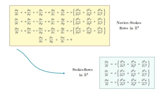
A Note on Stokes Approximations to Leray Solutions of the Incompressible Navier–Stokes Equations in ℝⁿ

Abstract

In the early 1980s it was well established that Leray solutions of the unforced Navier–Stokes equations in ${\mathbb{R}}^n$ decay in energy norm for large t. With the works of T. Miyakawa, M. Schonbek and others it is now known that the energy decay rate cannot in general be any faster than $t^{-(n+2)/4}$ and is typically much slower. In contrast, we show in this note that, given an arbitrary Leray solution $\mathit{u}(·,t)$, the difference of any two Stokes approximations to the Navier–Stokes flow $\mathit{u}(·,t)$ will always decay at least as fast as $t^{-(n+2)/4}$, no matter how slow the decay of ${\parallel \mathit{u}(·,t)\parallel }_{L^2\left({\mathbb{R}}^n\right)}$ might be.

1. Introduction

In this note, we derive an interesting new property regarding the large time behavior of Stokes flows approximating Leray solutions (as constructed by J. Leray in [1]) of the incompressible Navier–Stokes equations

$${\mathit{u}}_t+\mathit{u}·\nabla \mathit{u}+\nabla p=\nu ∆\mathit{u},\nabla ·\mathit{u}(·,t)=0,$$

(1)

$$\mathit{u}(·,0)={\mathit{u}}_0\in L_{\sigma }^2\left({\mathbb{R}}^n\right),$$

(2)

in dimension $2\le n\le 4$, where $\nu >0$ is constant and ${\displaystyle L_{\sigma }^2\left({\mathbb{R}}^n\right)}$ denotes the space of functions ${\displaystyle \mathbf{u}=({\mathrm{u}}_{{}_1},\dots ,{\mathrm{u}}_{{}_n})\in L^2\left({\mathbb{R}}^n\right)}$ with ${\displaystyle \nabla ·\mathbf{u}=0}$ in the distributional sense. Leray solutions to (1),(2) are mappings ${\displaystyle \mathit{u}(·,t)\in L^{\infty }((0,\infty ),L_{\sigma }^2\left({\mathbb{R}}^n\right))\cap L^2((0,\infty ),{\dot{H}}^1\left({\mathbb{R}}^n\right))}$ that are weakly continuous in $L^2\left({\mathbb{R}}^n\right)$ for all $t\ge 0$ and satisfy the Equation (1) in ${\mathbb{R}}^n\times (0,\infty )$ as distributions. Moreover, they satisfy the energy estimate [1,2,3,4,5,6]

$${\parallel \mathit{u}(·,t)\parallel }_{{}_{L^2\left({\mathbb{R}}^n\right)}}^2+2\nu {\int }_0^t{\parallel D\mathit{u}(·,s)\parallel }_{{}_{L^2\left({\mathbb{R}}^n\right)}}^{2}ds\le {\parallel {\mathit{u}}_0\parallel }_{{}_{L^2\left({\mathbb{R}}^n\right)}}^2$$

(3)

(for all $t\ge 0$), so that, in particular, ${\displaystyle \parallel \mathit{u}(·,t)-{\mathit{u}}_0{\parallel }_{L^2\left({\mathbb{R}}^n\right)}\to 0}$ as $t\searrow 0$. For $n\ge 3$, their uniqueness and exact regularity properties are still an open problem, but it is known that at the very least they must be smooth for large $t$: for some $t_{\ast }\ge 0$ (depending on the solution) we have ${\displaystyle \mathit{u}\in C^{\infty }({\mathbb{R}}^n\times (t_{\ast },\infty ))}$, and, for each $m\ge 0$,

$$\mathit{u}(·,t)\in C((t_{\ast },\infty ),H^m\left({\mathbb{R}}^n\right)),$$

(4)

as shown by Leray ([1], p. 246). Actually, we have

$$t_{\ast }\le 0.000465{\nu }^{-5}{\parallel {\mathit{u}}_0\parallel }_{{}_{L^2\left({\mathbb{R}}^3\right)}}^4(\mathrm{if}n=3)$$

(5)

and

$$t_{\ast }\le 0.002728{\nu }^{-3}{\parallel {\mathit{u}}_0\parallel }_{{}_{L^2\left({\mathbb{R}}^4\right)}}^2(\mathrm{if}n=4)$$

(6)

(see [7], Theorem A), with $t_{\ast }=0$ if $n=2$. For more on solution properties, see e.g., [1,2,3,4,5,6,8,9,10,11]. Here, we are particularly interested in the behavior for $t\gg 1$: it is now well known that, for every $m\ge 0$,

$$\underset{t\to \infty }{\lim }{t}^{m/2}{\parallel D^m\mathit{u}(·,t)\parallel }_{{}_{L^2\left({\mathbb{R}}^n\right)}}=0$$

(7)

(see e.g., [11,12,13,14,15,16,17,18,19,20,21]), where $\parallel D^m{\mathit{u}(·,t)\parallel }_{{}_{L^2\left({\mathbb{R}}^n\right)}}$ denotes the norm of $\mathit{u}(·,t)$ in ${\dot{H}}^m\left({\mathbb{R}}^n\right)$, that is,

$${\parallel \mathit{u}(·,t)\parallel }_{{}_{L^2\left({\mathbb{R}}^n\right)}}^2=\parallel u_{{}_1}{(·,t)\parallel }_{{}_{L^2\left({\mathbb{R}}^n\right)}}^2+\dots +{\parallel u_{{}_n}(·,t)\parallel }_{{}_{L^2\left({\mathbb{R}}^n\right)}}^2$$

(8)

if $m=0$ and

$$\parallel D^m{\mathit{u}(·,t)\parallel }_{{}_{L^2\left({\mathbb{R}}^n\right)}}^2=\sum _{i=1}^n\sum _{j_1=1}^n\cdots \sum _{j_{{}_m}=1}^n{\int }_{{}_{{\mathbb{R}}^n}}{\left|D_{j_{{}_1}}\cdots D_{j_{{}_m}}{u}_i(x,t)\right|}^{2}dx$$

(9)

if $m\ge 1$, where $D_j=\partial /\partial x_j$. For arbitrary initial values ${\mathit{u}}_0\in L_{\sigma }^2\left({\mathbb{R}}^n\right)$, the result (7) is all that can be obtained, but stronger additional assumptions may give that, for some $\alpha >0$, we actually have

$$\parallel D^m{\mathit{u}(·,t)\parallel }_{{}_{L^2\left({\mathbb{R}}^n\right)}}=O\left(t^{-\alpha -m/2}\right)$$

(10)

as $t\to \infty$, with the generic limitation $\alpha \le (n+2)/4$, see [8,22,23]. (For the exceptional case of faster decaying solutions, see [8,22,24,25].) Another point of interest is the large time behavior of the associated linear Stokes flows. In the case of (1), (2) these are given by solutions ${\displaystyle v(·,t)\in L^{\infty }([t_0,\infty ),L_{\sigma }^2\left({\mathbb{R}}^n\right))}$ of the linear heat flow problems

$${\mathit{v}}_t=\nu ∆\mathit{v},t>t_0,$$

(11)

$$\mathit{v}(·,t_0)=\mathit{u}(·,t_0),$$

(12)

for some given $t_0\ge 0$ (arbitrary). The solution is given by ${\displaystyle \mathit{v}(·,t)=e^{\nu ∆(t-t_0)}\mathit{u}(·,t_0)}$, where ${\displaystyle e^{\nu ∆\tau }}$, $\tau \ge 0$, is the heat semigroup. If $\alpha <(n+2)/4$, the error $\parallel D^m{(\mathit{u}-\mathit{v})(·,t)\parallel }_{L^2\left({\mathbb{R}}^n\right)}$ decays faster than the rate (10), so that the Stokes solutions (11), (12) give a useful approximation to the more complex Navier–Stokes flow $\mathit{u}(·,t)$ defined by the Equation (1).

Our contribution in this note is to point out that, for arbitrary Navier–Stokes flows (i.e., for arbitrary initial values ${\mathit{u}}_0\in L_{\sigma }^2\left({\mathbb{R}}^n\right)$), two distinct Stokes approximations $\mathit{v}(·,t),\tilde{\mathit{v}}(·,t)$ to $\mathit{u}(·,t)$ eventually become very closely similar in that we always have

$$\parallel D^m[\mathit{v}(·,t)-\tilde{\mathit{v}}(·,t)]{\parallel }_{{}_{L^2\left({\mathbb{R}}^n\right)}}=O\left(t^{-(n+2)/4-m/2}\right)$$

(13)

for large t. The precise statement reads as follows:

Theorem 1. 

Given $2\le n\le 4$ and ${\mathit{u}}_0\in L_{\sigma }^2\left({\mathbb{R}}^n\right)$, let ${\displaystyle \mathit{u}(·,t)\in L^{\infty }((0,\infty ),L_{\sigma }^2\left({\mathbb{R}}^n\right))\cap L^2((0,\infty ),}$${\dot{H}}^1\left({\mathbb{R}}^n\right))$ be any Leray solution to the Navier–Stokes equations $\left(1\right)$. Then, for any $0\le t_0<{\tilde{t}}_0$, we have

$$\parallel \mathit{v}(·,t)-\tilde{v}{(·,t)\parallel }_{{}_{L^2\left({\mathbb{R}}^n\right)}}\le K{\nu }^{-(n+2)/4}{\parallel \mathit{u}(·,0)\parallel }_{{}_{L^2\left({\mathbb{R}}^n\right)}}^2({\tilde{t}}_0-t_0){(t-{\tilde{t}}_0)}^{-(n+2)/4}$$

(14)

for all $t>{\tilde{t}}_0$, where $\mathit{v}(·,t)=e^{\nu ∆(t-t_0)}\mathit{u}(·,t_0)$ and $\tilde{v}(·,t)=e^{\nu ∆(t-{\tilde{t}}_0)}\mathit{u}(·,{\tilde{t}}_0)$ are the corresponding Stokes flows associated with the time instants $t_0$ and ${\tilde{t}}_0$, respectively, and $K={\left(4\pi \right)}^{-n/4}/\sqrt{e}$. Moreover, for any $m\ge 1$, we have

$$\parallel D^m[v(·,t)-\tilde{v}(·,t)]{\parallel }_{{}_{L^2\left({\mathbb{R}}^n\right)}}\le K(m,n){\nu }^{-(n+2)/4-m/2}{\parallel {\mathit{u}}_0\parallel }_{{}_{L^2\left({\mathbb{R}}^n\right)}}^2({\tilde{t}}_0-t_0){(t-{\tilde{t}}_0)}^{-(n+2)/4-m/2}$$

(15)

for all $t>{\tilde{t}}_0$, where the constant $K(m,n)$ depends only on $m,n$ (and not on $t_0,{\tilde{t}}_0,\nu ,{\mathit{u}}_0$ or the solution $\mathit{u}(·,t))$.

Remark 1. 

In dimension $n\ge 3$ it is not known whether Leray’s construction gives all (weak) solutions in the class $X=\{\mathit{u}(·,t)\in L^{\infty }((0,\infty ),L_{\sigma }^2\left({\mathbb{R}}^n\right))\cap L^2((0,\infty ),{\dot{H}}_{\sigma }^1\left({\mathbb{R}}^n\right)):\left(3\right)holds for all t>0\}$, the so-called Leray-Hopf solutions. In case it does not, it would be interesting to know if Theorem A remains valid for all Leray-Hopf solutions as well.

From (14), (15) and standard Sobolev imbeddings we obtain the following corollary regarding supnorm estimates.

Theorem 2. 

Given $2\le n\le 4$ and ${\mathit{u}}_0\in L_{\sigma }^2\left({\mathbb{R}}^n\right)$, let ${\displaystyle \mathit{u}(·,t)\in L^{\infty }((0,\infty ),L_{\sigma }^2\left({\mathbb{R}}^n\right))\cap L^2((0,\infty ),}$${\dot{H}}^1\left({\mathbb{R}}^n\right))$ be any Leray solution to the Navier–Stokes equations $\left(1\right)$. Then, for any $0\le t_0<{\tilde{t}}_0$, we have

$$\parallel D^m[\mathit{v}(·,t)-\tilde{\mathit{v}}(·,t)]{\parallel }_{{}_{L^{\infty }\left({\mathbb{R}}^n\right)}}\le G(m,n){\nu }^{-(n+2)/4-m/2-n/4}{\parallel \mathit{u}(·,0)\parallel }_{{}_{L^2\left({\mathbb{R}}^n\right)}}^2({\tilde{t}}_0-t_0){(t-{\tilde{t}}_0)}^{-(n+2)/4-m/2-n/4}$$

(16)

for all $t>{\tilde{t}}_0$ and every $m\ge 0$, where $\mathit{v}(·,t)=e^{\nu ∆(t-t_0)}\mathit{u}(·,t_0)$ and $\tilde{\mathit{v}}(·,t)=e^{\nu ∆(t-{\tilde{t}}_0)}\mathit{u}(·,{\tilde{t}}_0)$, and where $G(m,n)>0$ is some constant that depends only on $(m,n)$.

Remark 2. 

Earlier versions of (14) and (16) for $m=0$ were given in [26,27], but, as the results and analysis there were neither as sharp nor as complete as in the present discussion, they have now become obsolete.

The proof of Theorem 1 is developed in the next section, along with some necessary mathematical preliminaries. We end the discussion with some brief considerations in Section 3.

2. Proof of Theorem 1

We first recall Leray’s construction [1], as it will be needed in the proof of Theorem 1 if $n\ge 3$. (If $n=2$, the proof can be done directly from (1) by easily adapting the argument below.) For the construction of his solutions, Leray used an ingenious regularization procedure which we now review. Taking (any) ${\displaystyle G\in C_0^{\infty }\left({\mathbb{R}}^n\right)}$ nonnegative with ${\int }_{{\mathbb{R}}^n}G\left(x\right)dx=1$ and setting ${\displaystyle {\overline{\mathit{u}}}_{{}_{0,\delta }}(·)\in C^{\infty }\left({\mathbb{R}}^n\right)}$ by convolving ${\displaystyle {\mathit{u}}_0(·)}$ with ${\displaystyle G_{{}_{\delta }}\left(x\right)={\delta }^{-n}G(x/\delta )}$, $\delta >0$, one defines ${\displaystyle {\mathit{u}}_{{}_{\delta }},p_{{}_{\delta }}\in C^{\infty }({\mathbb{R}}^n\times [0,\infty ))}$ as the (unique, globally defined) classical $L^2$ solutions of the regularized equations

$${\displaystyle \frac{\partial }{\partial t}}{\mathit{u}}_{{}_{\delta }}+{\overline{\mathit{u}}}_{{}_{\delta }}(·,t)·\nabla {\mathit{u}}_{{}_{\delta }}+\nabla p_{{}_{\delta }}=∆{\mathit{u}}_{{}_{\delta }},\nabla ·{\mathit{u}}_{{}_{\delta }}(·,t)=0,$$

(17)

$${\mathit{u}}_{{}_{\delta }}(·,0)={\overline{\mathit{u}}}_{{}_{0,\delta }}:=G_{{}_{\delta }}\ast {\mathit{u}}_0\in \bigcap _{m=1}^{\infty }{H}^m\left({\mathbb{R}}^n\right),$$

(18)

where ${\displaystyle {\overline{\mathit{u}}}_{{}_{\delta }}(·,t):=G_{{}_{\delta }}\ast {\mathit{u}}_{{}_{\delta }}(·,t)}$. As shown by Leray, there is some sequence ${\displaystyle {\delta }^{\prime }\to 0}$ for which we have the weak convergence

$${\mathit{u}}_{{}_{{\delta }^{\prime }}}(·,t)\rightharpoonup \mathit{u}(·,t)\mathrm{as}{\delta }^{\prime }\to 0,\forall t\ge 0,$$

(19)

that is, ${\displaystyle {\mathit{u}}_{{}_{{\delta }^{\prime }}}(·,t)\to \mathit{u}(·,t)}$ weakly in $L^2\left({\mathbb{R}}^n\right)$, for every $t\ge 0$ (see [1], p. 237). This gives ${\displaystyle \mathit{u}(·,t)\in L^{\infty }((0,\infty ),L_{\sigma }^2\left({\mathbb{R}}^n\right))}$ ${\displaystyle \cap L^2((0,\infty ),{\dot{H}}^1\left({\mathbb{R}}^n\right))\cap C_w^0([0,\infty ),L^2\left({\mathbb{R}}^n\right))}$, with $\mathit{u}(·,t)$ continuous in $L^2$ at $t=0$ and solving the Navier–Stokes Equations (1) in distributional sense. Moreover, the energy inequality (3) is satisfied for all $t\ge 0$, so that, in particular,

$${\int }_0^{\infty }{\parallel D\mathit{u}(·,t)\parallel }_{{}_{L^2\left({\mathbb{R}}^n\right)}}^{2}dt\le {\displaystyle \frac{1}{2\nu }}{\parallel {\mathit{u}}_0\parallel }_{{}_{L^2\left({\mathbb{R}}^n\right)}}^2.$$

(20)

A similar estimate for the regularized solutions ${\displaystyle {\mathit{u}}_{{}_{\delta }}(·,t)}$ is also valid, since we have, from (17), (18) above, that

$$\parallel {\mathit{u}}_{{}_{\delta }}{(·,t)\parallel }_{{}_{L^2\left({\mathbb{R}}^n\right)}}^2+2\nu {\int }_0^t\parallel D{\mathit{u}}_{{}_{\delta }}{(·,s)\parallel }_{{}_{L^2\left({\mathbb{R}}^n\right)}}^{2}ds\le {\parallel {\mathit{u}}_0\parallel }_{{}_{L^2\left({\mathbb{R}}^n\right)}}^2$$

(21)

for all $t>0$ (and $\delta >0$ arbitrary). Another property shown in [1] is that ${\displaystyle \mathit{u}\in C^{\infty }({\mathbb{R}}^n\times (t_{\ast },\infty ))}$ for some $t_{\ast }$ $\ge 0$, with ${\displaystyle D^m\mathit{u}(·,t)\in C((t_{\ast },\infty ),L^2\left({\mathbb{R}}^n\right))}$ for each $m\ge 1$, cf.(4). The following result considers the Helmholtz projection of ${\displaystyle -\mathit{u}(·,t)·\nabla \mathit{u}(·,t)}$ into $L_{\sigma }^2\left({\mathbb{R}}^n\right)$, that is, the divergence-free field $\mathit{Q}(·,t)\in L_{\sigma }^2\left({\mathbb{R}}^n\right)$ given by

$$\mathit{Q}(·,t):=-\mathit{u}(·,t)·\nabla \mathit{u}(·,t)-\nabla p(·,t),\mathrm{a}.\mathrm{e}.t>0.$$

(22)

Of similar interest is the quantity ${\displaystyle {\mathit{Q}}_{{}_{\delta }}(·,t):=-{\overline{\mathit{u}}}_{{}_{\delta }}(·,t)·\nabla {\mathit{u}}_{{}_{\delta }}(·,t)-\nabla p_{{}_{\delta }}(·,t)}$, which will be important in Theorem 4 below.

Theorem 3. 

For almost every $s>0$ (and every $s\ge t_{\ast }$, with $t_{\ast }$ given in $\left(4\right)$ above), one has

$$\parallel e^{\nu ∆(t-s)}{\mathit{Q}(·,s)\parallel }_{{}_{L^2\left({\mathbb{R}}^n\right)}}\le K_{{}_1}\left(n\right){\nu }^{-n/4}{(t-s)}^{-n/4}{\parallel \mathit{u}(·,s)\parallel }_{{}_{L^2\left({\mathbb{R}}^n\right)}}{\parallel D\mathit{u}(·,s)\parallel }_{{}_{L^2\left({\mathbb{R}}^n\right)}}$$

(23)

and

$$\parallel e^{\nu ∆(t-s)}{\mathit{Q}(·,s)\parallel }_{{}_{L^2\left({\mathbb{R}}^n\right)}}\le K_{{}_2}\left(n\right){\nu }^{-(n+2)/4}{(t-s)}^{-(n+2)/4}{\parallel \mathit{u}(·,s)\parallel }_{{}_{L^2\left({\mathbb{R}}^n\right)}}^2$$

(24)

for all $t>s$, where $K_{{}_1}\left(n\right)={\left(8\pi \right)}^{-n/4}$ and $K_{{}_2}\left(n\right)={\left(4\pi \right)}^{-n/4}/\sqrt{e}$.

Proof. 

This is shown in [14], p. 236, using the Fourier transform. Here we give an alternative, direct argument in physical space: Let $\mathbb{P}$ be the Helmholtz projection. Since, by definition, $\mathbb{P}$ is an orthogonal projection in the Hilbert space of vector fields in $L^2$, we have ${\displaystyle {\parallel \mathbb{P}\mathit{f}\parallel }_{L^2}\le {\parallel \mathit{f}\parallel }_{L^2}}$ for any vector field in $L^2$. Hence we have ${\displaystyle \parallel e^{\nu ∆(t-s)}{\mathit{Q}(·,s)\parallel }_{L^2}=}$ $\parallel e^{\nu ∆(t-s)}{\mathbb{P}[\mathit{u}(·,s)·\nabla \mathit{u}(·,s)]\parallel }_{L^2}=$  ${\displaystyle \parallel \mathbb{P}[e^{\nu ∆(t-s)}(\mathit{u}(·,s)·\nabla \mathit{u}(·,s))]{\parallel }_{L^2}}$ $\le \parallel e^{\nu ∆(t-s)}{(\mathit{u}(·,s)·\nabla \mathit{u}(·,s))\parallel }_{L^2}\le {\parallel \mathsf{\Gamma }(t-s)\parallel }_{L^2}{\parallel \mathit{u}(·,s)·\nabla \mathit{u}(·,s)\parallel }_{L^1}$, where $\mathsf{\Gamma }$ denotes the heat kernel, so that ${\displaystyle \parallel e^{\nu ∆(t-s)}{\mathit{Q}(·,s)\parallel }_{L^2}\le {\parallel \mathsf{\Gamma }(t-s)\parallel }_{L^2}{\parallel \mathit{u}(·,s)\parallel }_{L^2}{\parallel \nabla \mathit{u}(·,s)\parallel }_{L^2}}$. This is (23). Similarly, ${\displaystyle \parallel e^{\nu ∆(t-s)}{\mathit{Q}(·,s)\parallel }_{L^2}}$  $\le {\sum }_{j=1}^n{\parallel \mathsf{\Gamma }(t-s)\ast D_j[{\mathit{u}}_{{}_j}(·,s)\mathit{u}(·,s)]\parallel }_{L^2}$ $={\sum }_{j=1}^n{\parallel D_j\mathsf{\Gamma }(t-s)\ast [u_{{}_j}(·,s)\mathit{u}(·,s)]\parallel }_{L^2}$  $\le {\sum }_{j=1}^n\parallel D_j{\mathsf{\Gamma }(t-s)\parallel }_{L^2}{\parallel {\mathit{u}}_{{}_j}(·,s)\mathit{u}(·,s)\parallel }_{L^1}$  $\le {\sum }_{j=1}^n\parallel D_j{\mathsf{\Gamma }(t-s)\parallel }_{L^2}\parallel u_{{}_j}{(·,s)\parallel }_{L^2}{\parallel \mathit{u}(·,s)\parallel }_{L^2}$, which gives (24), as claimed.  □

In a completely similar way, considering the solutions of the regularized Navier–Stokes Equations (17) and (18), one obtains

$$\parallel e^{\nu ∆(t-s)}{\mathit{Q}}_{{}_{\delta }}{(·,s)\parallel }_{{}_{L^2\left({\mathbb{R}}^n\right)}}\le K_{{}_1}\left(n\right){\nu }^{-n/4}{(t-s)}^{-n/4}\parallel {\mathit{u}}_{{}_{\delta }}{(·,s)\parallel }_{{}_{L^2\left({\mathbb{R}}^n\right)}}{\parallel D{\mathit{u}}_{{}_{\delta }}(·,s)\parallel }_{{}_{L^2\left({\mathbb{R}}^n\right)}}$$

(25)

and

$$\parallel e^{\nu ∆(t-s)}{\mathit{Q}}_{{}_{\delta }}{(·,s)\parallel }_{{}_{L^2\left({\mathbb{R}}^n\right)}}\le K_{{}_2}\left(n\right){\nu }^{-(n+2)/4}{(t-s)}^{-(n+2)/4}{\parallel {\mathit{u}}_{{}_{\delta }}(·,s)\parallel }_{{}_{L^2\left({\mathbb{R}}^n\right)}}^2$$

(26)

for all $t>s>0$, where the constants $K_{{}_1}\left(n\right),K_{{}_2}\left(n\right)$ are given in Theorem 3 and ${\displaystyle {\mathit{Q}}_{{}_{\delta }}(·,s)=-{\overline{\mathit{u}}}_{{}_{\delta }}(·,s)·\nabla {\mathit{u}}_{{}_{\delta }}(·,s)-\nabla p_{{}_{\delta }}(·,s)}$.

Theorem 4.  

Let $\mathit{u}(·,t)$, $t>0$, be any particular Leray solution to $\left(1\right)$. Given any pair of starting times ${\tilde{t}}_0>t_0\ge 0$, one has

$$\parallel v(·,t)-\tilde{v}{(·,t)\parallel }_{{}_{L^2\left({\mathbb{R}}^n\right)}}\le K_{{}_2}\left(n\right){\nu }^{-(n+2)/4}{\parallel \mathit{u}(·,0)\parallel }_{{}_{L^2\left({\mathbb{R}}^n\right)}}^{{}^2}({\tilde{t}}_0-t_0){(t-{\tilde{t}}_0)}^{-(n+2)/4}$$

(27)

for all $t>{\tilde{t}}_0$, where ${\displaystyle \mathit{v}(·,t)=e^{\nu ∆(t-t_0)}\mathit{u}(·,t_0)}$, ${\displaystyle \tilde{\mathit{v}}(·,t)=e^{\nu ∆(t-{\tilde{t}}_0)}\mathit{u}(·,{\tilde{t}}_0)}$ are the corresponding Stokes flows associated with $t_0$, ${\tilde{t}}_0$, respectively, and $K_{{}_2}\left(n\right)$ is given in Theorem 3 above, that is, $K_{{}_2}\left(n\right)={\left(4\pi \right)}^{-n/4}/\sqrt{e}$.

Proof. 

The following argument combines the Leray’s construction reviewed above with the usual strategy of handling nonlinear terms as a Duhamel-type correction. We begin by writing ${\displaystyle v(·,t)=e^{\nu ∆(t-t_0)}[\mathit{u}(·,t_0)-{\mathit{u}}_{{}_{\delta }}(·,t_0)]+e^{\nu ∆(t-t_0)}{\mathit{u}}_{{}_{\delta }}(·,t_0)}$, $t>t_0$, with ${\displaystyle {\mathit{u}}_{{}_{\delta }}(·,t)}$ given in (17), (18), $\delta >0$. Because

$${\mathit{u}}_{{}_{\delta }}(·,t_0)=e^{\nu ∆t_0}{\overline{\mathit{u}}}_{0,\delta }+{\int }_0^{t_0}{e}^{\nu ∆(t_0-s)}{\mathit{Q}}_{{}_{\delta }}(·,s)ds,$$

where ${\displaystyle {\overline{\mathit{u}}}_{{}_{0,\delta }}=G_{{}_{\delta }}\ast {\mathit{u}}_0}$ and ${\displaystyle {\mathit{Q}}_{{}_{\delta }}(·,s)=-{\overline{\mathit{u}}}_{{}_{\delta }}(·,s)·\nabla {\mathit{u}}_{{}_{\delta }}(·,s)-\nabla p_{{}_{\delta }}(·,s)}$, we get

$$\mathit{v}(·,t)=e^{\nu ∆(t-t_0)}[\mathit{u}(·,t_0)-{\mathit{u}}_{{}_{\delta }}(·,t_0)]+e^{\nu ∆t}{\overline{\mathit{u}}}_{0,\delta }+{\int }_0^{t_0}{e}^{\nu ∆(t-s)}{\mathit{Q}}_{{}_{\delta }}(·,s)ds,$$

for $t>t_0$. A similar expression holds for $\tilde{v}(·,t)$ as well, giving

$$\tilde{\mathit{v}}(·,t)-\mathit{v}(·,t)=e^{\nu ∆(t-{\tilde{t}}_0)}[\mathit{u}(·,{\tilde{t}}_0)-{\mathit{u}}_{{}_{\delta }}(·,{\tilde{t}}_0)]-e^{\nu ∆(t-t_0)}[\mathit{u}(·,t_0)-{\mathit{u}}_{{}_{\delta }}(·,t_0)]+{\int }_{t_0}^{{\tilde{t}}_0}{e}^{\nu ∆(t-s)}{\mathit{Q}}_{{}_{\delta }}(·,s)ds$$

for $t>{\tilde{t}}_0$. Therefore, given any ${\displaystyle \mathbb{K}\subset {\mathbb{R}}^n}$ compact, we get, for each $t>{\tilde{t}}_0$, $\delta >0$:

$$\begin{array}{cc}\hfill \parallel \tilde{\mathit{v}}{(·,t)-\mathit{v}(·,t)\parallel }_{{}_{L^2\left(\mathbb{K}\right)}}& \le J_{{}_{\delta }}\left(t\right)+{\int }_{t_0}^{{\tilde{t}}_0}{\parallel e^{\nu ∆(t-s)}{\mathit{Q}}_{{}_{\delta }}(·,s)\parallel }_{{}_{L^2\left(\mathbb{K}\right)}}ds\hfill \\ \hfill & \le J_{{}_{\delta }}\left(t\right)+K_{{}_2}\left(n\right){\nu }^{-(n+2)/4}{\int }_{t_0}^{{\tilde{t}}_0}{(t-s)}^{-(n+2)/4}{\parallel {\mathit{u}}_{{}_{\delta }}(·,s)\parallel }_{{}_{L^2\left({\mathbb{R}}^n\right)}}^{2}ds\hfill \\ \hfill & \le J_{{}_{\delta }}\left(t\right)+K_{{}_2}\left(n\right){\nu }^{-(n+2)/4}{\parallel {\mathit{u}}_0\parallel }_{{}_{L^2\left({\mathbb{R}}^n\right)}}^{{}^2}({\tilde{t}}_0-t_0){(t-{\tilde{t}}_0)}^{-(n+2)/4}\hfill \end{array}$$

by (21) and (26), where $K_{{}_2}\left(n\right)={\left(4\pi \right)}^{-n/4}/\sqrt{e}$ and

$$J_{{}_{\delta }}\left(t\right)=\parallel e^{\nu ∆(t-{\tilde{t}}_0)}[\mathit{u}(·,{\tilde{t}}_0)-{\mathit{u}}_{{}_{\delta }}(·,{\tilde{t}}_0)]{\parallel }_{L^2\left(\mathbb{K}\right)}+{\parallel e^{\nu ∆(t-t_0)}[\mathit{u}(·,t_0)-{\mathit{u}}_{{}_{\delta }}(·,t_0)]\parallel }_{L^2\left(\mathbb{K}\right)}.$$

Taking $\delta ={\delta }^{\prime }\to 0$ according to (19), we get $J_{{}_{\delta }}\left(t\right)\to 0$, since, by Lebesgue’s Dominated Convergence Theorem and (19), we have, for any $\sigma ,\tau >0$: ${\displaystyle \parallel e^{\nu ∆\tau }[\mathit{u}(·,\sigma )-{\mathit{u}}_{{}_{{\delta }^{\prime }}}(·,\sigma )]{\parallel }_{{}_{L^2\left(\mathbb{K}\right)}}\to 0}$ as ${\displaystyle {\delta }^{\prime }\to 0}$. This gives (27), as claimed.  □

In particular, we obtained (14). This, in turn, gives (15) using well known estimates of the heat operator, or, alternatively, by applying to (14) the direct method introduced in [28] to derive upper estimates in the spaces ${\dot{H}}^m\left({\mathbb{R}}^n\right)$. This completes the proof of Theorem 1.

3. Concluding Remarks

The main results of this note (namely, Theorems 1 and 2) show the somewhat surprising fact that the difference of any two Stokes approximations to an arbitrarily given Leray solution of the Navier–Stokes system (1), (2) will always decay as $t\to \infty$ at least as fast as the fastest decaying Leray flows in general, no matter how slow the particular Leray solution at hand might be decaying. This is an interesting theoretical finding about Stokes flows in ${\mathbb{R}}^n$, which are important approximations for Navier–Stokes flows. On the more practical side, it sheds some additional light on the quality of these approximations. For example, it shows that M. Wiegner’s estimates ([20], Theorem (c), p. 305) on the large time size of the error $\parallel \mathit{u}(·,t)-e^{\nu ∆t}{\mathit{u}}_0{\parallel }_{L^2\left({\mathbb{R}}^n\right)}$ apply more generally to the error of any Stokes approximation of $\mathit{u}(·,t)$, and so forth.

References

1. Leray, J. Essai sur le mouvement d’un fluide visqueux emplissant l’espace. Acta Math. 1934, 63, 193–248. [Google Scholar] [CrossRef]
2. Kreiss, H.-O.; Lorenz, J. Initial-Boundary Value Problems and the Navier-Stokes Equations; Academic Press: New York, NY, USA, 1989. [Google Scholar]
3. Ladyzhenskaya, O.A. The Mathematical Theory of Viscous Incompressible Flows, 2nd ed.; Gordon and Breach: New York, NY, USA, 1969. [Google Scholar]
4. Robinson, J.C.; Rodrigo, J.L.; Sadowski, W. The Three-Dimensional Navier-Stokes Equations; Cambridge University Press: Cambridge, UK, 2016. [Google Scholar]
5. Sohr, H. The Navier-Stokes Equations; Birkhäuser: Basel, Switzerland, 2001. [Google Scholar]
6. Temam, R. Navier-Stokes Equations: Theory and Numerical Analysis; AMS/Chelsea: Providence, RI, USA, 1984. [Google Scholar]
7. Silva, P.B.E.; Zingano, J.P.; Zingano, P.R. A note on the regularity time of Leray solutions to the Navier-Stokes equations. J. Math. Fluid Mech. 2019, 21, 8. [Google Scholar] [CrossRef]
8. Brandolese, L.; Schonbek, M.E. Large time behavior of the Navier-Stokes flow. In Handbook of Mathematical Analysis in Mechanics of Viscous Fluids, Part I; Giga, Y., Novotny, A., Eds.; Springer: New York, NY, USA, 2018. [Google Scholar]
9. Galdi, G.P. An introduction to the Navier-Stokes initial-boundary problem. In Fundamental Directions in Mathematical Fluid Dynamics; Galdi, G.P., Heywood, J.G., Rannacher, R., Eds.; Birkhauser: Basel, Switzerland, 2000; pp. 1–70. [Google Scholar]
10. Lorenz, J.; Zingano, P.R. The Navier-Stokes equations for incompressible flows: Solution properties at potential blow-up times. Bol. Soc. Paran. Mat. 2015, 35, 127–158. [Google Scholar]
11. Niche, C.J.; Schonbek, M.E. Decay characterization of solutions to dissipative equations. J. Lond. Math. Soc. 2015, 91, 573–595. [Google Scholar] [CrossRef] [Green Version]
12. Kajikiya, R.; Miyakawa, T. On the L2 decay of weak solutions of the Navier-Stokes equations in ℝn. Math. Z. 1986, 192, 135–148. [Google Scholar] [CrossRef]
13. Kato, T. Strong Lp-solutions of the Navier-Stokes equations in ℝm, with applications to weak solutions. Math. Z. 1984, 187, 471–480. [Google Scholar] [CrossRef]
14. Kreiss, H.-O.; Hagstrom, T.; Lorenz, J.; Zingano, P.R. Decay in time of incompressible flows. J. Math. Fluid Mech. 2003, 5, 231–244. [Google Scholar] [CrossRef]
15. Masuda, K. Weak solutions of the Navier-Stokes equations. Tôhoku Math. J. 1984, 36, 623–646. [Google Scholar] [CrossRef]
16. Oliver, M.; Titi, E.S. Remark on the rate of decay of higher order derivatives for solutions to the Navier-Stokes equations in ℝn. J. Funct. Anal. 2000, 172, 1–18. [Google Scholar] [CrossRef] [Green Version]
17. Schonbek, M.E. Large time behaviour of solutions of the Navier-Stokes equations. Commun. Partial Differ. Equ. 1986, 11, 733–763. [Google Scholar] [CrossRef]
18. Schonbek, M.E. Large time behaviour of solutions to the Navier-Stokes equations in Hm spaces. Commun. Partial Differ. Equ. 1995, 20, 103–117. [Google Scholar] [CrossRef]
19. Schonbek, M.E.; Wiegner, M. On the decay of higher-order norms of the solutions of Navier-Stokes equations. Proc. R. Soc. Edinb. Sect. A 1996, 126, 677–685. [Google Scholar] [CrossRef]
20. Wiegner, M. Decay results for weak solutions of the Navier-Stokes equations on ℝn. J. Lond. Math. Soc. 1987, 35, 303–313. [Google Scholar] [CrossRef]
21. Zhou, Y. A remark on the decay of solutions to the 3-D Navier-Stokes equations. Math. Methods Appl. Sci. 2007, 30, 1223–1229. [Google Scholar] [CrossRef]
22. Gallay, T.; Wayne, C.E. Long-time asymptotics of the Navier-Stokes and vorticity equations on ℝ3. Philos. Trans. R. Soc. Lond. 2002, 360, 2155–2188. [Google Scholar] [CrossRef] [PubMed] [Green Version]
23. Miyakawa, T.; Schonbek, M.E. On optimal decay rates for weak solutions to the Navier-Stokes equations in ℝn. Math. Bohem. 2001, 126, 443–455. [Google Scholar] [CrossRef]
24. Brandolese, L. Space-time decay of Navier-Stokes flows invariant under rotations. Math. Ann. 2004, 329, 685–706. [Google Scholar] [CrossRef] [Green Version]
25. Gallay, T.; Wayne, C.E. Invariant manifolds and the long-time asymptotics of the Navier-Stokes and vorticity equations on ℝ2. Arch. Rat. Mech. Anal. 2002, 163, 209–258. [Google Scholar] [CrossRef] [Green Version]
26. Rigelo, J.C.; Schütz, L.; Zingano, J.P.; Zingano, P.R. Leray’s problem for the Navier-Stokes equations revisited. C. R. Math. 2016, 354, 503–509. [Google Scholar] [CrossRef]
27. Schütz, L.; Zingano, J.P.; Zingano, P.R. On the supnorm form of Leray’s problem for the incompressible Navier-Stokes equations. J. Math. Phys. 2015, 56, 071504. [Google Scholar] [CrossRef] [Green Version]
28. Hagstrom, T.; Lorenz, J.; Zingano, J.P.; Zingano, P.R. On two new inequalities for Leray solutions of the Navier-Stokes equations in ℝn. J. Math. Anal. Appl. 2020, 483, 123601. [Google Scholar] [CrossRef]
Publisher’s Note: MDPI stays neutral with regard to jurisdictional claims in published maps and institutional affiliations.