Numerical Simulations of Flows in a Cerebral Aneurysm Using the Lattice Boltzmann Method with the Half-Way and Interpolated Bounce-Back Schemes

Abstract

Lattice Boltzmann simulations and a velocity measurement of flows in a cerebral aneurysm reconstructed from MRA (magnetic resonance angiography) images of an actual aneurysm were carried out and the numerical results obtained using the bounce-back schemes were compared with the experimental data to discuss the effects of the numerical treatment of the no-slip boundary condition of the complex boundary shape of the aneurysm on the predictions. The conclusions obtained are as follows: (1) measured data of the velocity in the aneurysm model useful for validation of numerical methods were obtained, (2) the numerical stability of the quadratic interpolated bounce-back scheme (QBB) in the flow simulation of the cerebral aneurysm is lower than those of the half-way bounce-back (HBB) and the linearly interpolated bounce-back (LBB) schemes, (3) the flow structures predicted using HBB and LBB are comparable and agree well with the experimental data, and (4) the fluctuations of the wall shear stress (WSS), i.e., the oscillatory shear index (OSI), can be well predicted even with the jaggy wall representation of HBB, whereas the magnitude of WSS predicted with HBB tends to be smaller than that with LBB.

1. Introduction

A cerebral aneurysm is a disease in which the blood vessel of a cerebral artery is deformed into a saccular geometry. Rupture of cerebral aneurysms induces subarachnoid hemorrhage, which is an extremely serious disease with a high probability of death or poor prognosis, and therefore, it is important to understand the mechanisms of growth and rupture of the cerebral aneurysms. Although it has been pointed out that hemodynamic parameters, e.g., the wall-shear stress (WSS) acting on the artery wall, relate with the growth and rupture mechanisms [1,2], our knowledge on the mechanisms is still insufficient.

Computational fluid dynamics (CFD) is expected as a powerful tool to analyze fluid flows inside cerebral aneurysms. Foutrakis et al. [3] used artificial aneurysm models, which were two-dimensional channels with branches and convex geometries, to numerically investigate the characteristics of flows in the aneurysms. Valencia et al. [4] carried out three-dimensional simulations of flows in artificial aneurysm models and discussed the effects of the angle of connection between the aneurysm and the artery on the flow. These numerical studies were carried out using the artificial aneurysm models. On the other hand, numerical simulations with aneurysm models reconstructed from actual patient data have been carried out since the early 2000’s [5,6,7]. Due to the complex shapes of actual cerebral aneurysms, it is desired to simply model the boundary condition at the artery wall. Since the lattice Boltzmann method (LBM) [8] can easily deal with such complex boundary shapes by using the bounce-back schemes, we developed a numerical method based on LBM for simulating blood flows in cerebral aneurysms in our previous studies [9,10,11].

The LBM predicts fluid flows based on the motion of imaginary fluid particles and the no-slip condition at the solid wall is simulated by the bounce-back motion of the particles. The half-way bounce-back scheme (HBB) [12] is the simplest, but the solid boundary is represented by a stepwise shape along the computational grid lines even for curved boundaries. On the other hand, the linearly interpolated bounce-back scheme (LBB) and the quadratic interpolated bounce-back scheme (QBB) deal with the boundary shape more accurately [13]. The HBB and LBB have been used in simulations of flows in cerebral aneurysms [14,15]. However the validation of HBB and LBB were usually carried out only for simple geometries [13] and the effects of the boundary model on the predicted flows in cerebral aneurysms have not been discussed in detail. The QBB uses the quadratic interpolation of the velocity distribution function. Therefore QBB is expected to be more accurate than LBB, which is based on the linear interpolation. Sanjeevi et al. [16] have however pointed out that QBB is less stable compared with LBB.

In our previous study [10], we investigated the effects of the collision models (single-, two- and multiple-relaxation time collision models) and the viscous stress model on numerical predictions of flows in cerebral aneurysms. However, the effects of the numerical treatment of the wall boundary condition on numerical predictions for the complex geometries were not discussed. For validation of numerical simulations with the complex shape of an actual cerebral aneurysm, experimental data must be obtained with the same channel geometry. In this study, we made a cerebral aneurysm model reconstructed from MRA (magnetic resonance angiography) images of an actual aneurysm for velocity measurement and lattice Boltzmann simulations and compared numerical results obtained using the bounce-back schemes with the experimental data to discuss the effects of the numerical treatment of the no-slip boundary condition on the predictions. The cerebral aneurysm model for the experiment was produced by making use of 3D printing from a STL (stereolithography) mesh of the cerebral aneurysm, which was also used to generate the scalar field (the signed-distance function) representing the boundary shape in the simulation to assure the same geometries in the experiment and the simulation.

2. Numerical Method

2.1. Lattice Boltzmann Method

The outline of the numerical method is described in the following. The details can be found in our previous paper [10]. The numerical method is based on LBM, in which fluid flows are simulated by the motion of imaginary fluid particles. The motion of imaginary fluid particles is governed by the following lattice Boltzmann equation:

$$f_i\left(\mathit{x}+{\mathit{c}}_i\Delta t,t+\Delta t\right) = f_i\left(\mathit{x},t\right)+\Omega$$

(1)

where $f(\mathit{x},t)$ is the velocity distribution function of particles with the velocity $\mathit{c}$ at the position $\mathit{x}$ and the time t, $\Delta t$ is the time step size, $\Omega$ is the collision term, and the subscript i represents the direction of the particle velocity. The D3Q19 discrete velocity model for isothermal incompressible flows is adopted, i.e., $i=0,1,2,\cdots ,18$. The multiple-relaxation time collision model (MRT) [17] is used for $\Omega$:

$$\Omega =-M^{-1}S\left(\mathit{m}-{\mathit{m}}^{eq}\right)$$

(2)

where M is the matrix transforming f into its moment vector $\mathit{m}(=M\mathit{f})$, $\mathit{f}$ is the vectorial representation of $f_i$, and S is the relaxation parameter matrix. The ${\mathit{m}}^{eq}$ is the moment vector for the equilibrium distribution functions $f^{eq}$, which are given by

$$f_i^{eq}=\rho w_i\left[1+3{\mathit{c}}_i·\mathit{u}+\frac{9{\left({\mathit{c}}_i·\mathit{u}\right)}^2}{2}-\frac{3\mathit{u}·\mathit{u}}{2}\right]$$

(3)

where $w_i$ is the weighting function, $\mathit{u}$ is the fluid velocity, and $\rho$ is the fluid density. The $\rho$ and $\mathit{u}$ are given by

$$\rho =\sum _{i=0}^{18}{f}_i$$

(4)

$$\mathit{u}=\frac{1}{\rho }\sum _{i=0}^{18}{\mathit{c}}_i{f}_i$$

(5)

2.2. Boundary Condition

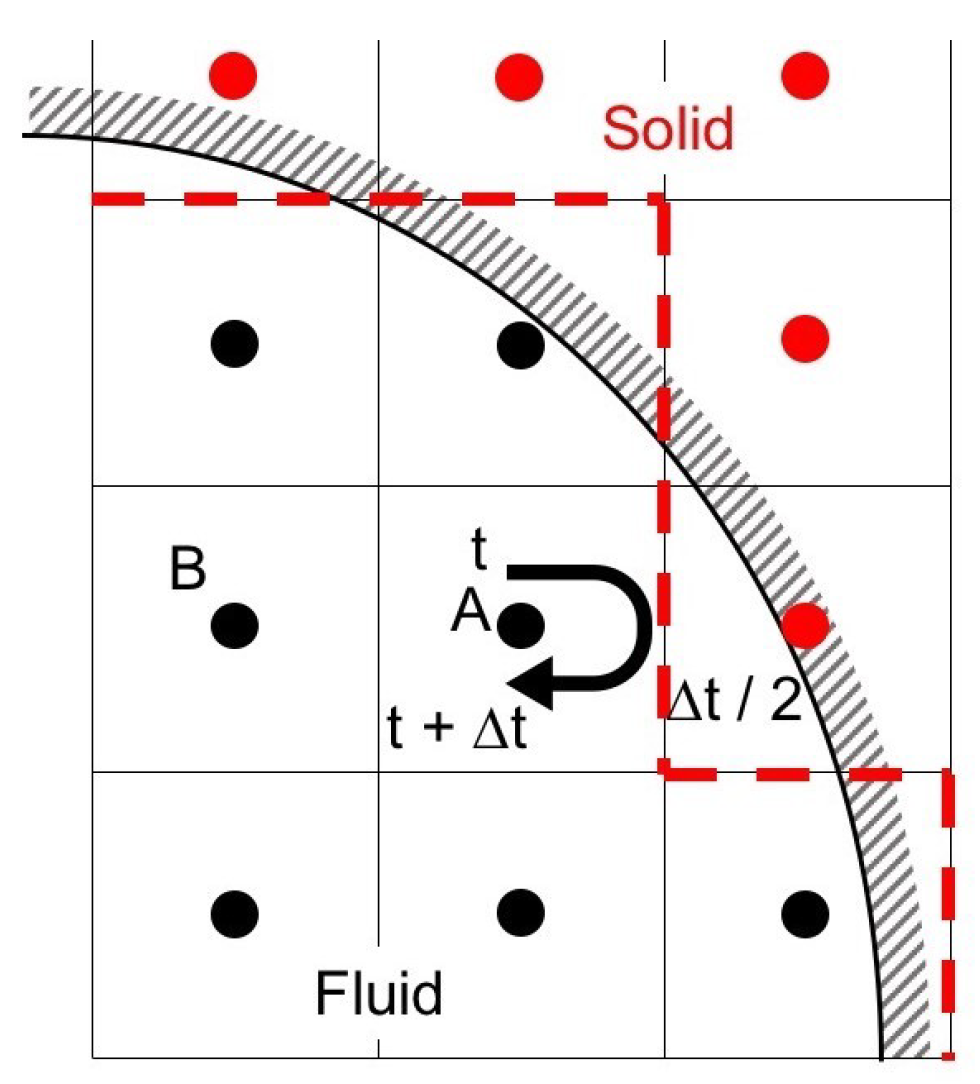
The LBM often uses the bounce-back scheme, which assumes that particles collide with the solid wall and bounce back in the direction opposite to the original direction so as to impose the no-slip boundary condition. In HBB, particles travel from a cell center toward the wall during the time duration $\Delta t/2$, and collide with the wall at $t+\Delta t/2$. Then, the particles return to the cell center at $t+\Delta t$. Therefore

$$f_{\overline{i}}\left(\mathit{x},t+\Delta t\right) = f_i\left(\mathit{x},t\right)$$

(6)

where $\overline{i}$ is the opposite direction of the i direction. Figure 1 shows an example of the applications of HBB to a curved boundary. The curved wall is represented by the dashed line in HBB. The jaggy representation of the curved boundary possibly deteriorates the accuracy of predictions in the vicinity of the wall, especially when the spatial resolution is low.

Figure 1. Half-way bounce-back scheme.

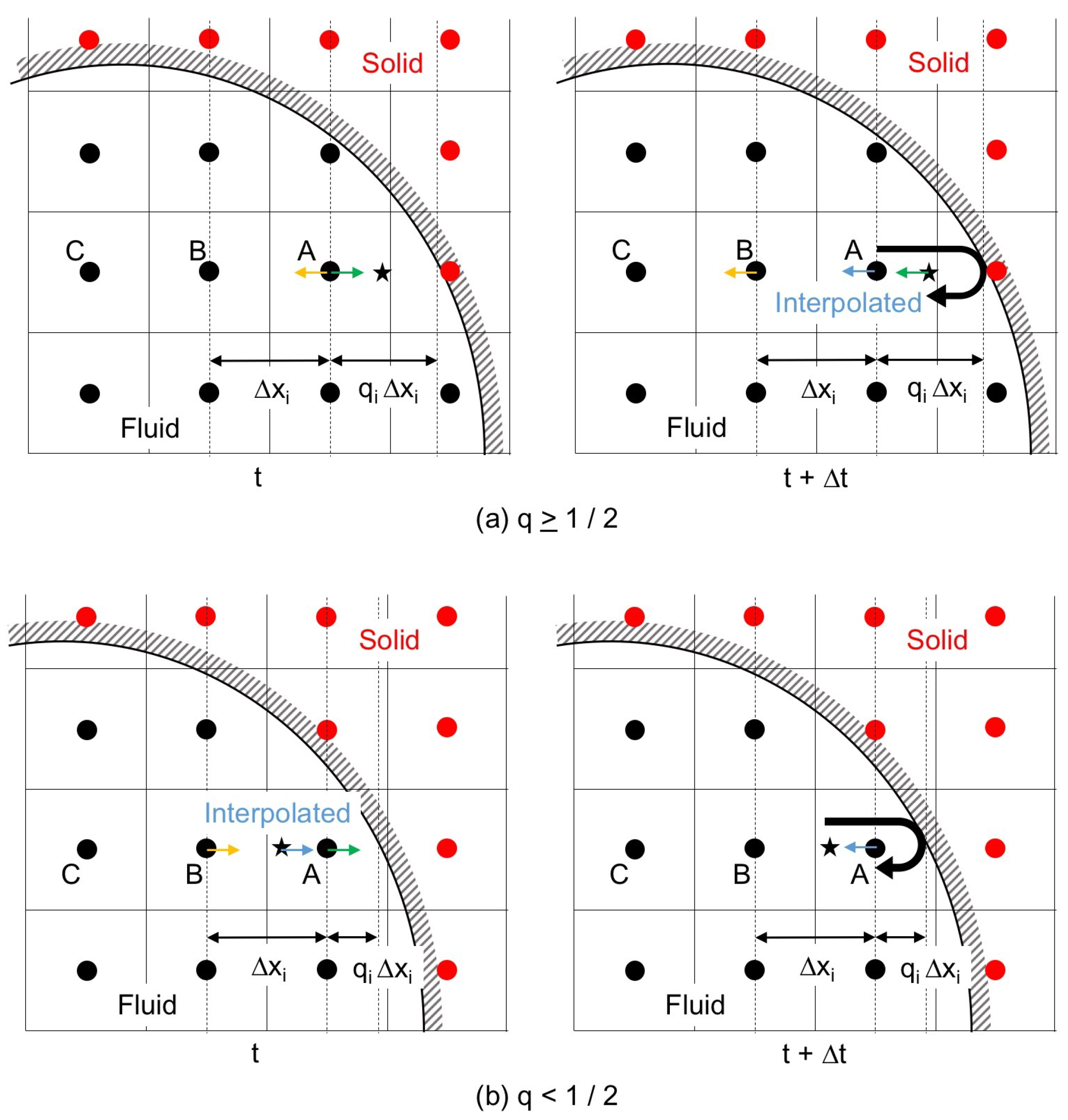
The interpolated bounce-back scheme (IBB), which interpolates $f_i$ by taking into account the ratio, $q_i$, of the distance between the wall and the cell center to the grid spacing $\Delta x$, was proposed to improve the accuracy of the boundary representation [13] as shown in Figure 2. The linearly interpolated bounce-back scheme (LBB) is IBB with the first-order interpolation, and $f_i$ directing towards the wall at ${\mathit{x}}_A$ and t (Figure 2) is changed after the time duration $\Delta t$ as

$$f_{\overline{i}}\left({\mathit{x}}_A,t+\Delta t\right)=\left\{\begin{array}{cc}\frac{1}{2q_i}{f}_i\left({\mathit{x}}_A,t\right)+\frac{2q_i-1}{2q_i}{f}_{\overline{i}}\left({\mathit{x}}_A,t\right)\hfill & \mathrm{for}{q}_i\ge 1/2\hfill \\ 2q_i{f}_i\left({\mathit{x}}_A,t\right)+\left(1-2q_i\right)f_i\left({\mathit{x}}_B,t\right)\hfill & \mathrm{for}{q}_i<1/2\hfill \end{array}\right.$$

(7)

The IBB with the second-order interpolation is the following quadratic interpolated bounce-back scheme (QBB):

$$f_{\overline{i}}\left({\mathit{x}}_A,t+\Delta t\right)=\left\{\begin{array}{cc}\frac{2q_i-1}{q_i}{f}_{\overline{i}}\left({\mathit{x}}_A,t\right)+\frac{1}{q_i\left(2q_i+1\right)}{f}_i\left({\mathit{x}}_A,t\right)+\frac{1-2q_i}{1+2q_i}{f}_{\overline{i}}\left({\mathit{x}}_B,t\right)\hfill & \mathrm{for}{q}_i\ge 1/2\hfill \\ q_i\left(1+2q_i\right)f_i\left({\mathit{x}}_A,t\right)+\left(1-4q_i^2\right)f_i\left({\mathit{x}}_B,t\right)-q_i\left(1-2q_i\right)f_i\left({\mathit{x}}_C,t\right)\hfill & \mathrm{for}{q}_i<1/2\hfill \end{array}\right.$$

(8)

where the subscripts A, B and C denote the cells in Figure 2.

Figure 2. Interpolated bounce-back scheme; (a) interpolation after the collision with the solid wall, $q\ge 1/2$; and (b) interpolation before the collision, $q<1/2$.

2.3. Cerebral Aneurysm Model

STL data of a cerebral aneurysm is generated from MRA images as shown in Figure 3, where the STL mesh is a collection of triangular elements. The STL data are imported into our in-house LBM code, AN2WER [9,10,11], and are used to reconstruct the signed-distance function (level set function) [18], $\psi$, which is used to evaluate the distance fraction, $q_i$, in IBB. The $\psi$ is the negative distance from the wall in the solid region, whereas $\psi$ is the positive distance in the fluid region, and therefore, the zero-level set, $\psi =0$, represents the wall. The $\psi$ is reconstructed as follows. For the Cth computational cell at ${\mathit{x}}_C$, the distance from the wall given by the eth triangular element is given by

$${\psi }_{e\to C}^L=\left({\mathit{x}}_C-{\mathit{x}}_e\right)·{\mathit{n}}_e$$

(9)

where ${\mathit{x}}_e$ and ${\mathit{n}}_e$ are the position vector and the unit normal of the eth element, respectively. Contributions from all the elements near ${\mathit{x}}_C$ are collected to obtain $\psi \left({\mathit{x}}_C\right)$ using the following weighting average [19]:

$$\psi \left({\mathit{x}}_C\right)=\frac{{\sum }_e{\psi }_{e\to C}^L{|{\mathit{x}}_C-{\mathit{x}}_e|}^{-p}}{{\sum }_e{|{\mathit{x}}_C-{\mathit{x}}_e|}^{-p}}$$

(10)

where the power, p, for the weight is set to seven. Figure 4 shows the level set function reconstructed from the STL data in Figure 3.

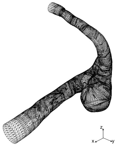
Figure 3. STL mesh of cerebral aneurysm model generated from MRA images.

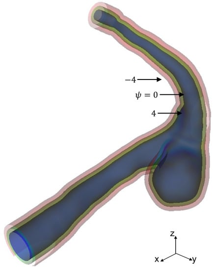
Figure 4. Level set function for aneurysm surface representation.

By making use of $\psi$, $q_i$ in Equations (7) and (8) are given by

$$q_i=\frac{|\psi \left(\mathit{x}\right)|}{|\psi \left(\mathit{x}\right)|+|\psi \left(\mathit{x}+{\mathit{c}}_i\Delta t\right)|}$$

(11)

3. Experimental

3.1. Experimental Setup

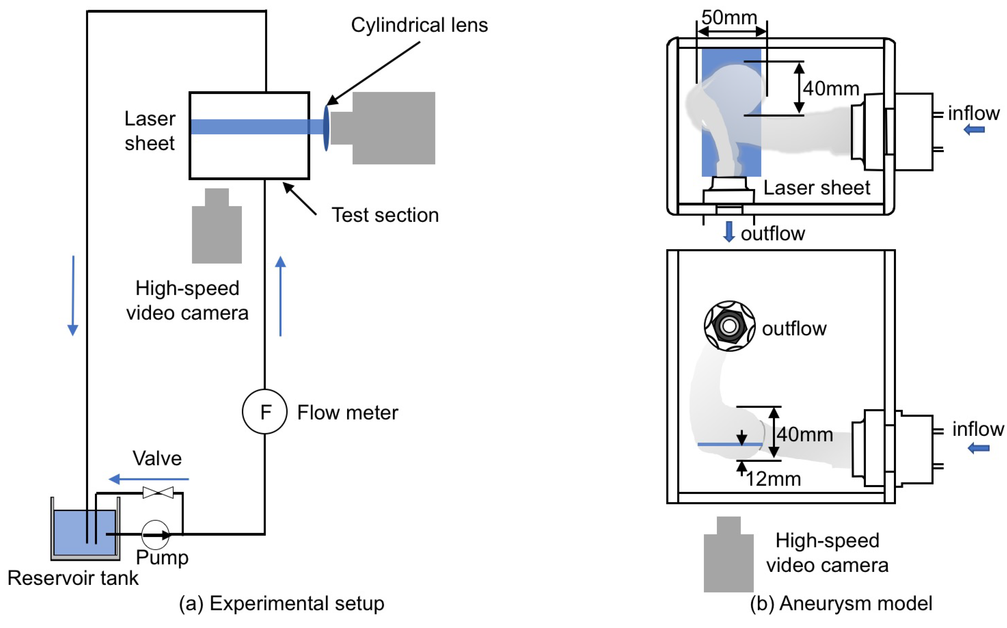
Figure 5a shows the experimental setup, which consists of the test section, the reservoir tank (TRUSCO, F-3GR), the pump (IWAKI, MD-15R-N), the flow meter (NIPPON FROW CELL, FDT-H-5) and the laser light source (KENTEC, LDB2W-H (wavelength: 450 nm)). The liquid phase was supplied from the tank to the test section using the pump and returned to the tank after flowing the test section.

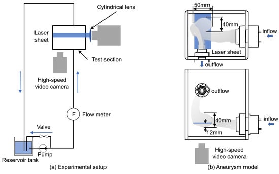
Figure 5. Experimental equipment. (a) experimental setup; (b) aneurysm model made using 3D printing.

The test section (Figure 5b) was the cerebral aneurysm model (Figure 3) made by using 3D printing (Yasojima Proceed Co. Ltd., Kobe, Japan). The aneurysm model had the single inlet and outlet, and its dimensions in the width, depth and height were approximately 50, 40 and 40 mm, respectively. The aneurysm models in the experiment and the simulation had the same geometry since the same STL data were used. The material was the transparent resin (stratasys, VeroClear). The resolution of the 3D printing was 30 $\mathsf{\mu }$m per layer. The model was produced from two parts for smoothing the inner surface. UV-cured coating was applied after smoothing, so that the model boundary was rigid. The test section was surrounded by the rectangular box of transparent acrylic resin and the box was filled with the liquid phase. For the liquid phase, silicone oil (Shin-Etsu Silicone, KF-56A (Newtonian fluid)) was used for index matching [20]. The liquid phase supplied by the pump was flowed into the aneurysm model through a horizontal circular pipe of 24 mm inner diameter, D, and 450 mm length (hydraulic entrance section). The temperature of the liquid phase was $24.8\pm 1 °\mathrm{C}$ and the flow rate was $2.38$ L/min. The Reynolds number defined by

$$Re=\frac{\rho UD}{\mu }$$

(12)

was 150, which is the typical value in cerebral arteries [21], where U is the mean velocity ($0.088$ m/s), and $\mu$ is the liquid viscosity.

The velocity field was measured using the spatial filter velocimetry (SFV) [22] as described in the next section. The laser beam generated by the light source passed through the cylindrical lens to form a laser sheet for SFV. The position of the laser sheet was 12 mm above the bottom of the aneurysm. The thickness of the laser sheet was about $1.0$ mm. Tracer particles, SiC (the specific gravity 1.69, the average particle diameter 3 $\mathsf{\mu }$m), were added in the oil for the velocity measurement. The high-speed video camera (Redlake, Motion Pro X-3) and the camera lens (Nikon, 60 mm f/2.8D) were used to take particle images.

3.2. Spatial Filter Velocimetry

The SFV was used to measure the velocity in the aneurysm. The outline of SFV for the measurement of the velocity component in the x direction is as follows. Grayscale images of tracer particles are obtained by using a high-speed video camera. The images are divided into smaller pieces, which are called the interrogation areas (IA). The mean particle velocity in IA can be obtained by evaluating the change in the intensity of grayscale value due to the motion of particles. In order to evaluate the change in the intensity, the following spatial filter, $\mathcal{F}$, is applied to the grayscale values:

$$\mathcal{F}(x,t)=cos\left(kx+\omega t\right)$$

(13)

where k is the wave number of the spatial filter, and $\omega$ is the angular frequency. The integrated intensity, $I\left(t_n\right)$, in IA of the nth frame image is given by

$$I\left(t_n\right)=\sum _{l,m}\mathcal{F}(x_l,t_n)g_{lm}$$

(14)

where the subscripts l and m are indices of the pixels in the x and y directions, respectively, and $g_{lm}$ is the grayscale value of the pixel at $(x_l,y_m)$. The I is normalized as

$$\tilde{I}\left(t_n\right)=\frac{I\left(t_n\right)-m_I}{{\sigma }_I}$$

(15)

The $m_I$ and ${\sigma }_I$ are given by

$$m_I=\frac{1}{N}\sum _{n=1}^{N}I\left(t_n\right)$$

(16)

$${\sigma }_I=\sqrt{\frac{1}{N-1}\sum _{n=1}^N{\left(I\left(t_n\right)-m_I\right)}^2}$$

(17)

where N is the total number of images. The peak frequency, $f_p$, of $\tilde{I}$ is obtained by applying the wavelet transformation, and the mean velocity is then evaluated as

$$v=(f_p-f_s)L$$

(18)

where the shift frequency, $f_s$, is given by

$$f_s=\frac{\omega }{2\pi }$$

(19)

and the filter pitch, L, is given by

$$L=\frac{2\pi }{k}$$

(20)

The $f_s$ is introduced to detect particles moving in the $-x$ direction. The velocity component in the y direction is obtained in the same manner. See Hosokawa et al. [22] for more details.

4. Results and Discussion

4.1. Inflow Condition

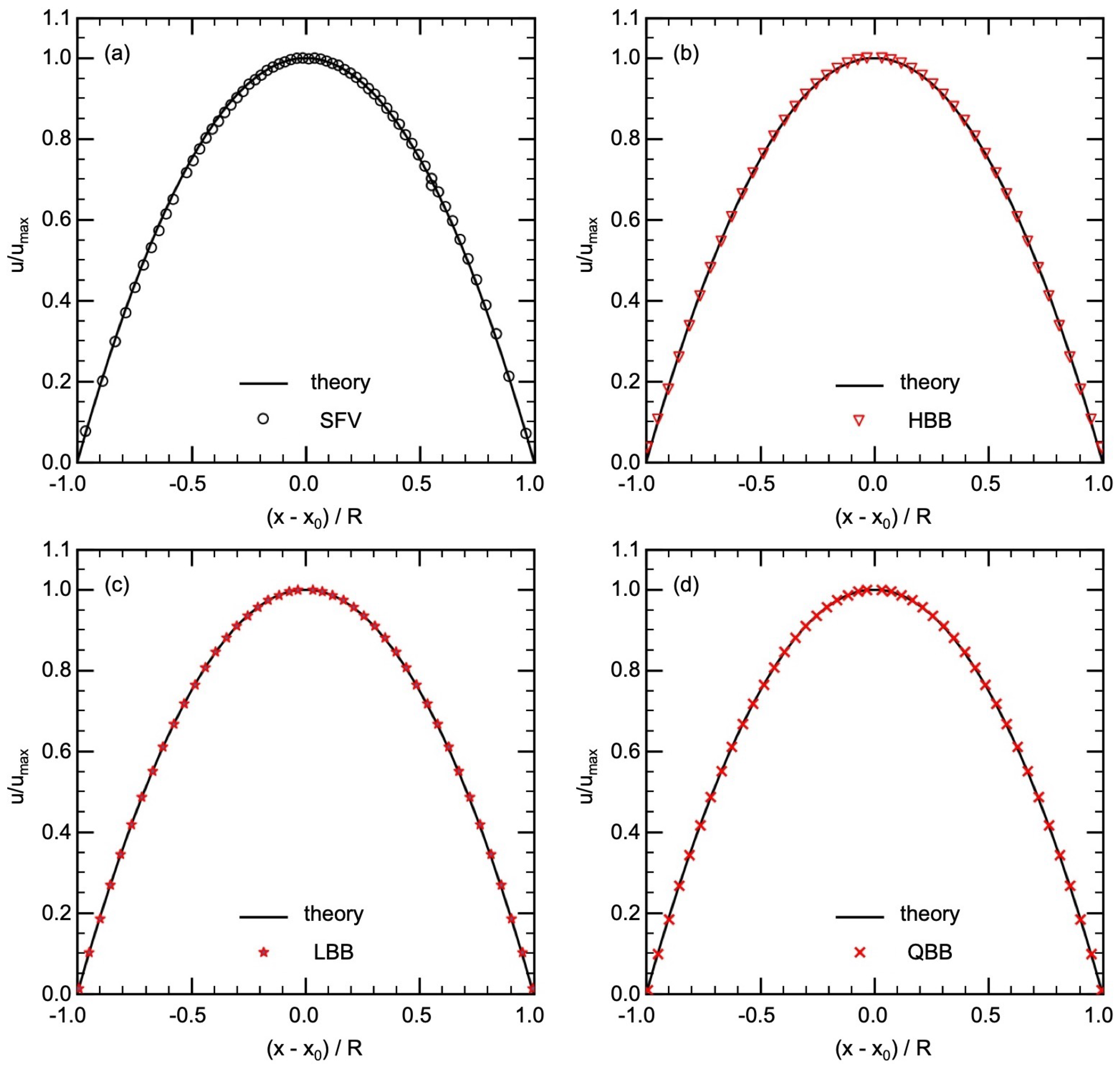
A velocity measurement of the flow in the circular pipe (hydraulic entrance section) was carried out to obtain the velocity distribution at the inlet of the test section, which will also be used as the inlet condition in the numerical simulations of flows in the aneurysm. Table 1 shows the parameters for SFV. The measurement positions of each velocity data were corrected by taking into account the refraction at the pipe surface. Figure 6a shows a comparison between the measured data of the time-averaged streamwise velocity u and the Poiseuille distribution, i.e., $u/u_{max}=[1-{(r/R)}^2]$, where $u_{max}$ is the maximum velocity at the pipe center, r is the radial coordinate, and R is the pipe radius. The data agree well with the laminar velocity profile, confirming that the flow was fully-developed in the entrance section and the inlet condition in the numerical simulations of flows in the aneurysm could be simply given by the Poiseuille distribution.

Table 1. Experimental conditions of SFV at inlet area.

Frame rate [frame/s]	3000
Number of images [frame]	16,000
Filter pitch [pix]	5
Spatial resolution [mm/pix]	0.053
Shift frequency [Hz]	0

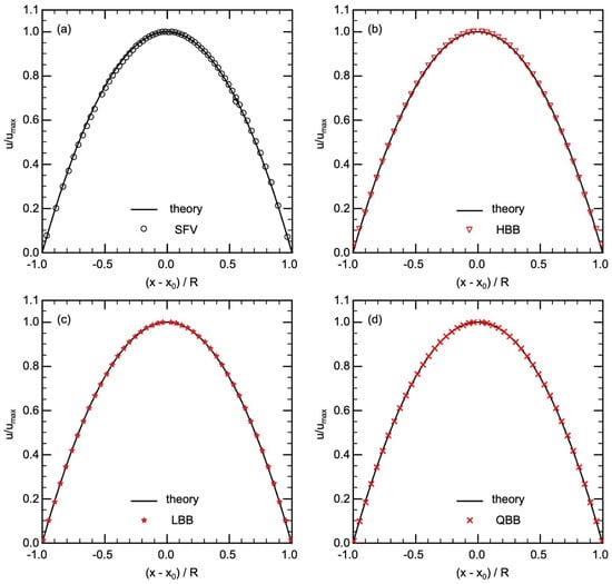
Figure 6. Comparison of velocity in pipe flow between theory and (a) SFV, (b) HBB, (c) LBB, (d) QBB (x is the position of the velocity data, $x_0$ is the position of the center of the pipe and R is the radius of the pipe).

Laminar flows in the circular pipe were predicted using HBB, LBB and QBB. Table 2 shows the numerical conditions. The fluid was Newtonian and the Reynolds number was the same as in the experiment. The relaxation time, $\tau$, was $0.517$ and the liquid kinematic viscosity in the LBM simulation was given as $\nu =(\tau -1/2)/3$ for $\Delta x=\Delta t=1$. The number of cells in the streamwise direction was 400. The computational domain for the cross section was $48\times 48$ cells, whereas D was 10% smaller than the domain size, i.e., $D=43.2$ cells.

Table 2. Numerical conditions of pipe flow simulation.

Number of cells	$400\times 48\times 48$
Inlet velocity U	0.02
Length scale D	43.2
Reynolds number $Re$	150
Relaxation time $\tau$	0.517

Streamwise velocities predicted using HBB, LBB and QBB are shown in Figure 6b–d, respectively. In all the cases, the predictions agree well with the laminar velocity profile. The spatial resolution of $43.2$ for D is therefore sufficient to obtain a good result even with the jaggy boundary representation of HBB. However, in the cells closest to the pipe wall, the predicted velocity in HBB is slightly larger than the analytical value. The deviations of the predicted u in those cells from the analytical value (0.0087) were 0.027, 0.0052 and 0.00011 for HBB, LBB and QBB, respectively. The distance between the pipe axis and the wall on the line passing through the axis is $22.0$ in HBB, which is slightly larger than the actual radius $D/2=21.6$ due to the stepwise representation of the wall. The fluid domain is therefore bit wider on this line, which resulted in the predicted velocity larger than the analytical value. On the other hand, the smaller errors in the velocities obtained with LBB and QBB clearly show that the interpolation calculation treats the position of the wall more accurately.

4.2. Steady Flow in Cerebral Aneurysm

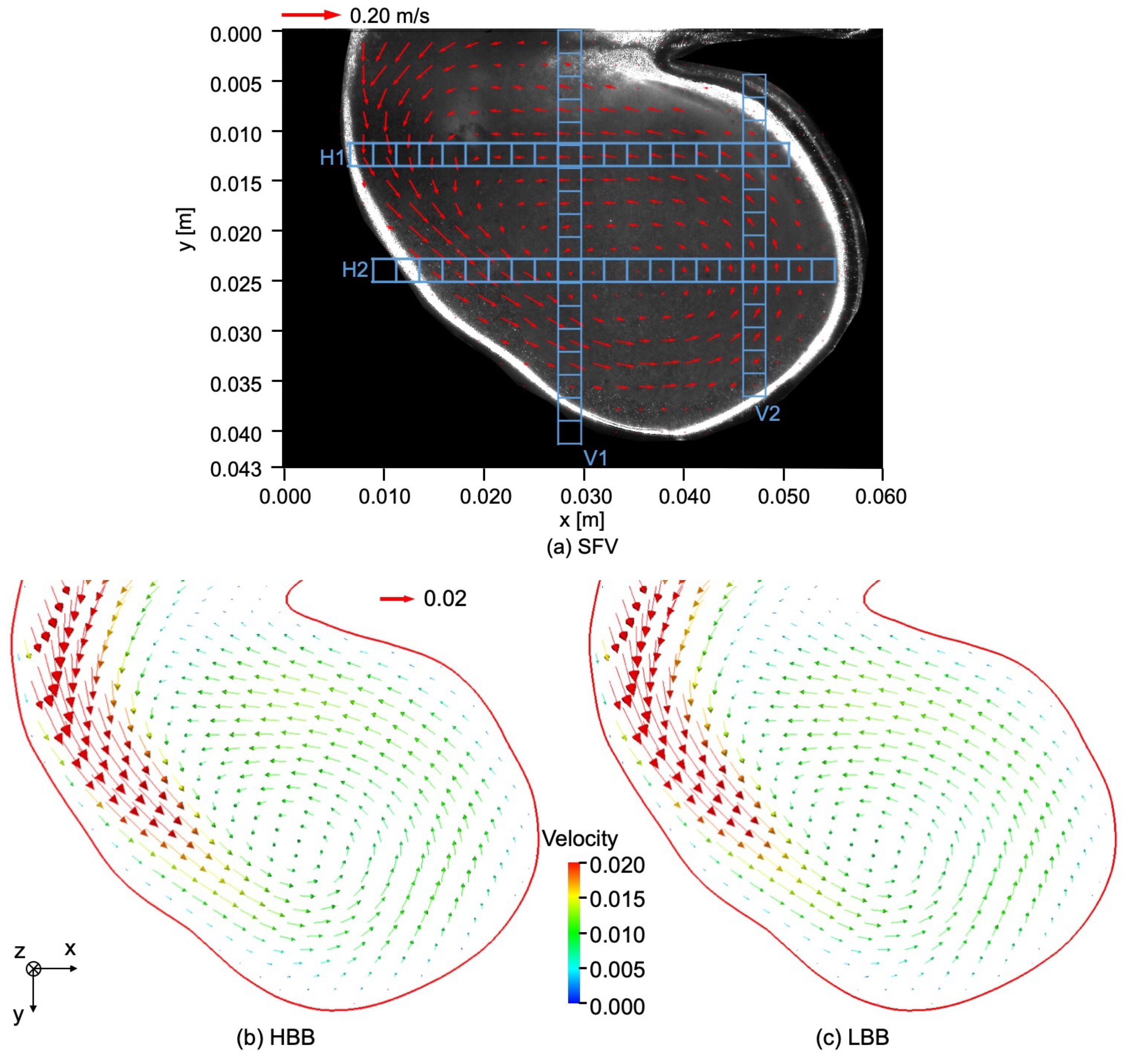
Figure 7a shows the velocity field in the cerebral aneurysm model measured by using SFV, the parameters of which are shown in Table 3. The liquid flows from the left top region of the image into the aneurysm along the left-side wall and a vortical structure is formed inside it. The center of the vortical structure is close to that of the aneurysm. The magnitude of the velocity inside the aneurysm is much smaller than the mean velocity at the inlet of the test section, i.e., $U=0.088$ m/s.

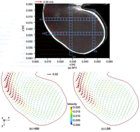
Figure 7. Comparison of velocity fields between (a) SFV, (b) HBB and (c) LBB.

Table 3. Parameters of SFV for aneurysm model.

Frame rate [frame/s]	1000
Filter pitch [pix]	11
Spatial resolution [mm/pix]	0.052
Shift frequency [Hz]	110.0

Numerical simulations of flows in the cerebral aneurysm model were carried out. Table 4 shows the numerical conditions. Although the simulations were carried out using HBB, LBB and QBB, the simulation with QBB was unstable under the given conditions and a steady state solution could not be obtained. The numerical stability of QBB is therefore lower than the others in the present case. A similar trend was also confirmed by Sanjeevi et al. [16], i.e., for a high $Re$ flow in a simpler channel geometry with a strong pressure gradient, QBB tends to be less stable than LBB.

Table 4. Numerical conditions for flow in aneurysm.

Number of cells ($N_x\times N_y\times N_z$)	$162\times 217\times 226$
Number of cells for D	40
Relaxation time $\tau$	0.516

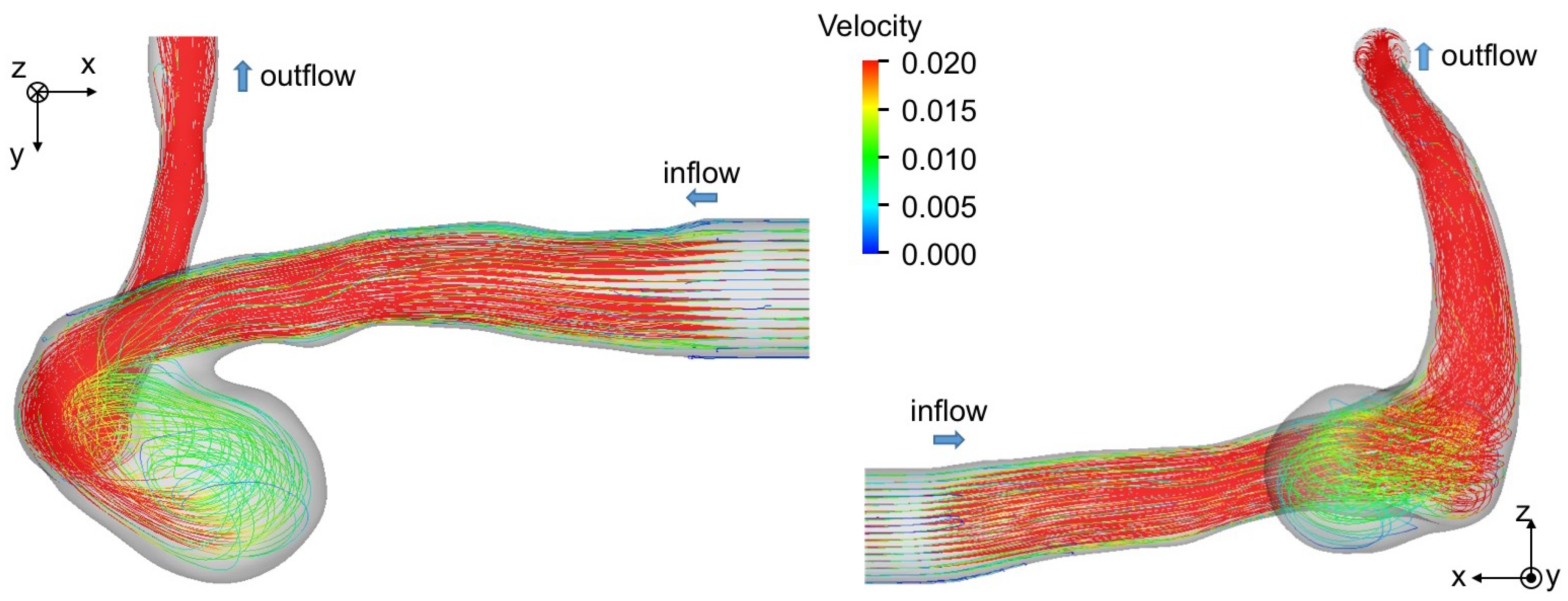
Figure 7b,c show the velocity fields predicted using HBB and LBB, respectively. The number of the vectors was reduced in the figures for visualization purpose. Being similar to the data, the liquid enters into the aneurysm model along the left side wall and a vortical structure is formed inside the aneurysm in the predictions, which confirms that both HBB and LBB give qualitatively reasonable results. The differences between the results of HBB and LBB seem small, and therefore, from the qualitative point of view, the effects of the numerical treatment of the no-slip boundary condition on the predictions of the flow structure in the aneurysm are not significant. Figure 8 shows streamlines obtained using LBB to understand the flow structure in the whole aneurysm model. The liquid from the circular inlet flows almost rectilinearly in the main artery section, whereas the streamlines are largely bended due to the interaction with the aneurysm wall, which corresponds to the left side wall of the aneurysm shown in Figure 7. Swirling motion is then formed inside the aneurysm and the streamlines direct toward the artery outlet.

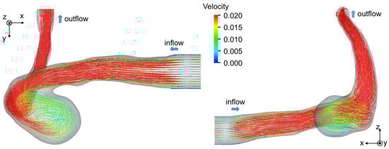
Figure 8. Flow structure in cerebral artery. The streamlines are drawn by using the result of LBB.

The measured and predicted velocities at the positions indicated by the blue squares on the lines, H1 (horizontal), H2, V1 (vertical) and V2, shown in Figure 7a are compared in the following to discuss the validity of the predictions in more detail. Figure 9 shows the measured velocities (the open circles) on H1, where $v_x$ and $v_y$ are the x and y components of the velocities normalized by the mean velocity at the inlet. On H1 in Figure 7a, the flow directs downward ($+y$ direction) for $x<0.02$ m due to the liquid inflow from the main artery, whereas for larger x the liquid in the vortical structure flows from the right to the left ($-x$ direction). Therefore the values of $v_y$ for $x<0.02$ m are positive and large and, for larger x, $v_x$ has negative values and its magnitude is much larger than that of $v_y$. The $v_x$ and $v_y$ of HBB and LBB agree well with those of SFV though some deviations appear, especially for $x<0.025$ m. No significant differences are found in the predictions of HBB and LBB, that is, the sum of the absolute differences between the velocity components of HBB and LBB on each line are less than several percent of the sum of the absolute value of the velocity components.

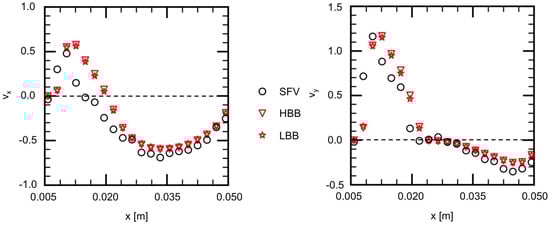
Figure 9. Comparison of velocity components between measured (SFV), HBB and LBB (line H1).

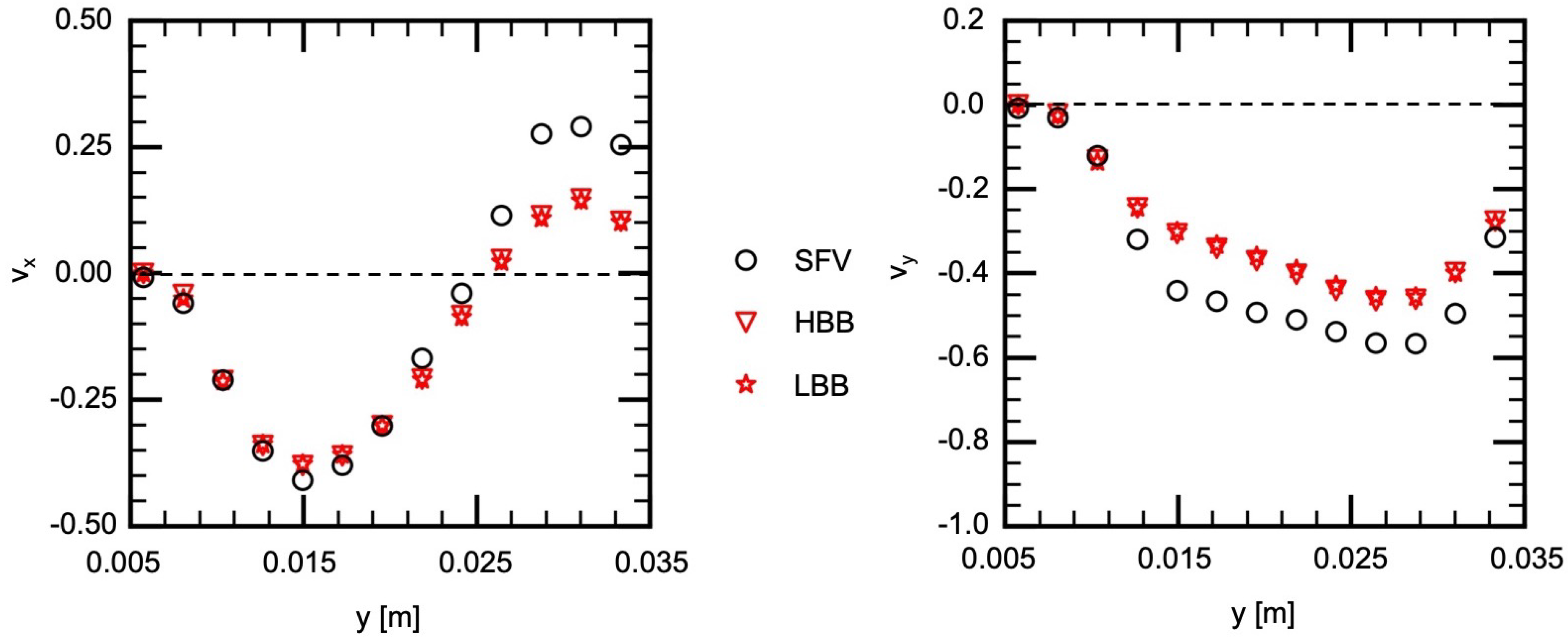
Figure 10 shows the velocities on H2, which passes the center of the vortical structure ($x\sim 0.03$ m) and therefore the velocity components change their signs near that position. The liquid flow along the left side wall exhibits large velocities and passes H2 almost diagonally. Therefore the magnitudes of $v_x$ and $v_y$ are large in the small x region. The predictions of HBB and LBB reproduce well the velocity profile though they are somewhat smaller than those of SFV.

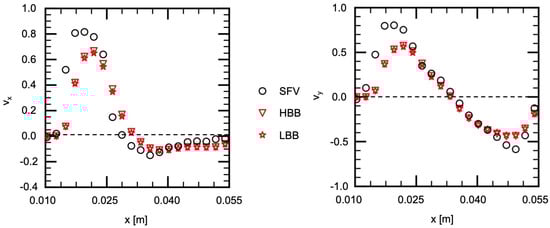
Figure 10. Comparison of velocity components between measured (SFV), HBB and LBB (line H2).

Figure 11 and Figure 12 show $v_x$ and $v_y$ on V1 and V2, respectively. Being similar to the velocity components on H1 and H2, the velocity profiles, in other words, the vortical structure in the cerebral aneurysm model, are well predicted using HBB and LBB, and the predictions of HBB and LBB are not so different.

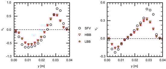
Figure 11. Comparison of velocity components between measured (SFV), HBB and LBB (line V1).

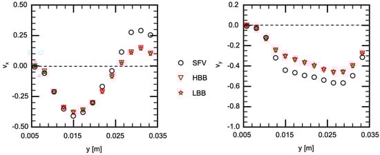
Figure 12. Comparison of velocity components between measured (SFV), HBB and LBB (line V2).

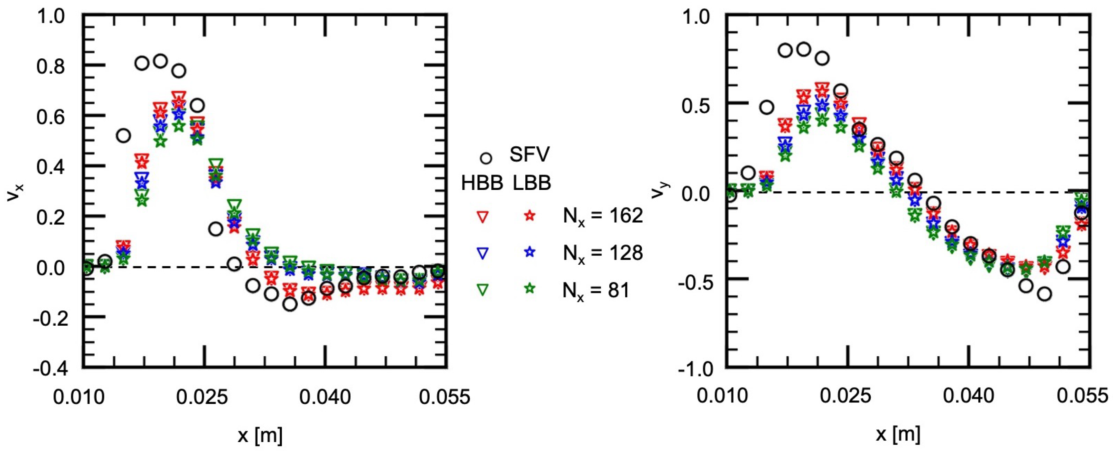
As discussed above, the velocities in the aneurysm model of HBB and LBB agree with the data and the differences between the predictions of HBB and LBB are small, which confirms that both numerical treatments of the wall can give reasonable predictions for the present complex geometry and the effects of the wall boundary treatment on the predicted flow structure in the aneurysm are small. We should however examine also the effects of the wall boundary treatment at lower spatial resolutions since the predictions of HBB would be worse than those of LBB as the spatial resolution decreases due to the stepwise representation of the wall. We therefore carried out the simulation with lower spatial resolutions. The spatial resolutions additionally tested were $N_x\times N_y\times N_z=128\times 172\times 178$ and $81\times 109\times 114$. The other conditions were the same as in the previous simulation. The numbers of cells for D were 31 and 20 for the former and the latter, respectively, and $\tau$ were $0.5125$ and $0.5079$. It should be noted that a spatial resolution lower than $N_x=81$ was also tested, but a numerical instability took place and a steady state solution could not be obtained.

Figure 13 shows the comparison of the velocity components, $v_x$ and $v_y$, between $N_x=162$, 128 and 81. The flow characteristics in the experiment are reproduced well with HBB and LBB even at the lowest spatial resolution although the decrease in the spatial resolution slightly deteriorates the prediction. Interestingly the prediction of HBB is not so different from that of LBB even at the lowest spatial resolution, and therefore, the jaggy representation of the aneurysm wall is still acceptable to reproduce the flow structure.

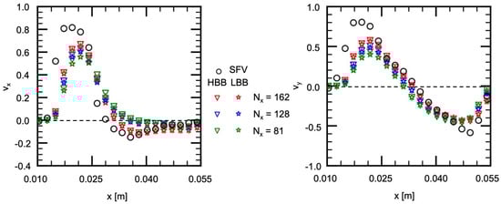
Figure 13. Comparison of velocity components between HBB and LBB at lower spatial resolutions (line H2).

4.3. Wall Shear Stress and Oscillatory Shear Index

Some hemodynamic parameters, e.g., the time-averaged wall shear stress (TAWSS), the oscillatory shear index (OSI) and so on, have been proposed to describe the growth and rupture mechanisms of cerebral aneurysms so far, where TAWSS is the magnitude of WSS acting on an aneurysm wall averaged for the single cardiac cycle, T, and OSI is an indicator representing the degree of directional change of WSS during T. In our previous study [11], we reported that thin aneurysm wall regions of un-ruptured cerebral aneurysms are correlated with OSI at a high probability, i.e., a low OSI region in numerical predictions corresponds to a thin wall region observed in an endovascular surgery. The TAWSS also showed correlations with the thickness of the aneurysm wall, i.e., a high TAWSS region corresponds to a thin wall region, whereas OSI would be more effective than TAWSS.

We therefore carried out numerical simulations of flows in the cerebral aneurysm model with an unsteady inlet condition and evaluated TAWSS and OSI to discuss the effects of the wall boundary treatment on these hemodynamic parameters. The Casson model [23] was used to account for the shear-thinning characteristics [10,24]. The inlet condition was time-dependent to roughly mimic the change in the flow rate during T, i.e., the flow rate increased at the early stage of T until it reached the peak value (the contraction period), and then, it decreased and returned to the initial value (the dilation period) (see Kimura et al. [9] for the detail).

The instantaneous wall shear stress vector, ${\tau }_W$, is given by

$${\tau }_W=(\mathit{I}-\mathit{n}\mathit{n})·(\mu \nabla \mathit{u})\approx \mu \frac{(\mathit{I}-\mathit{n}\mathit{n})·\mathit{u}\left(\mathit{x}\right)}{\psi \left(\mathit{x}\right)}$$

(21)

where $\mathit{x}$ is the position of the center of a cell closest to the wall, $\mathit{I}$ is the unit tensor and $\mathit{n}$ is the unit normal to the wall given by

$$\mathit{n}=\frac{\nabla \psi }{|\nabla \psi |}$$

(22)

The TAWSS is given by

$$\mathrm{TAWSS}=\frac{1}{T}{\int }_0^T\left|{\tau }_W\right|dt$$

(23)

The OSI is a hemodynamic parameter that describes the fluctuation of the WSS vector during T and is given by [25]

$$\mathrm{OSI}=\frac{1}{2}\left(1-\frac{|{\int }_0^T{\tau }_{W}dt|}{{\int }_0^T\left|{\tau }_W\right|dt}\right)$$

(24)

The spatial resolutions were $N_x=162$, $N_x=128$ and $N_x=81$, $Re$ was 150, and the Bingham number, $Bi$, was 0.1, where

$$Bi=\frac{{\tau }_{0}D}{{\mu }_{P}U}$$

(25)

Here ${\tau }_0$ is the yield stress and ${\mu }_P$ is the reference viscosity. The time average of U was set to 0.02.

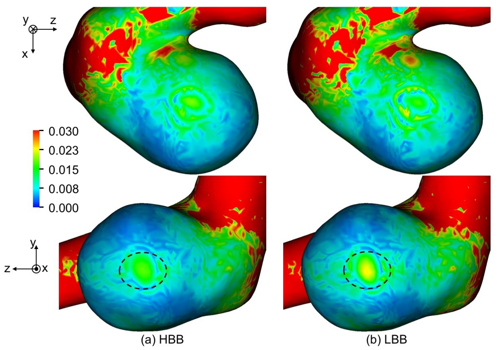
Figure 14a,b show TAWSS predicted using HBB and LBB, respectively, with $N_x=162$. The distributions of TAWSS of HBB and LBB are similar although TAWSS of HBB is somewhat smaller than that of LBB in some areas, e.g., the region indicated by the dashed oval in the figure. Table 5 shows TAWSS averaged for the aneurysm. The TAWSSs of HBB are about 11% smaller than those of LBB at all the spatial resolutions. The TAWSS depending on the wall boundary model implies that the velocity vectors near the aneurysm wall are different in HBB and LBB though the velocity profiles in the entire aneurysm are almost the same as shown in the previous section. Table 6 shows the mean values of the magnitude of the velocity component tangent to the wall, $v_t=|(\mathit{I}-\mathit{n}\mathit{n})·\mathit{u}\left(\mathit{x}\right)|$, in the computational cells closest to the aneurysm wall. Being similar to TAWSS, the mean tangential velocity of HBB is smaller than that of LBB regardless of the spatial resolution. Therefore the smaller TAWSS in HBB is due to the smaller velocity magnitude in the near wall region.

Figure 14. Comparison of TAWSS between (a) HBB and (b) LBB (the spatial resolution: $N_x=162$; TAWSS is normalized with $\rho U^2/2$).

Table 5. TAWSS and OSI averaged in aneurysm (TAWSS is normalized with $\rho U^2/2$).

	${\mathit{N}}_{\mathit{x}}=162$		${\mathit{N}}_{\mathit{x}}=128$		${\mathit{N}}_{\mathit{x}}=81$
	TAWSS	OSI	TAWSS	OSI	TAWSS	OSI
HBB	0.0108	0.0222	0.0127	0.0200	0.00975	0.0217
LBB	0.0123	0.0221	0.0143	0.0198	0.0109	0.0203

Table 6. Mean $v_t$ in aneurysm (normalized with U).

${\mathit{N}}_{\mathit{x}}$	162	128	81
HBB	0.00390	0.00709	0.00617
LBB	0.00488	0.00866	0.00770

Figure 15 shows the predicted OSI of $N_x=162$, where the maximum value of OSI for visualization is set to 0.01 since regions of $\mathrm{OSI}<0.01$ were confirmed to have correlations with thin wall regions [11]. The distributions of OSI predicted with HBB and LBB show only a little difference. The mean OSIs for the aneurysm are shown in Table 5; the values of HBB and LBB are very similar. The same trend was also seen for $N_x=128$ and $N_x=81$. Hence HBB can predict fluctuations of WSS as well as LBB in spite of the jaggy representation of the curved boundary.

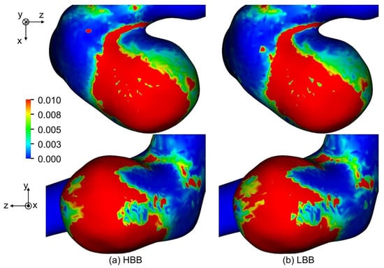
Figure 15. Comparison of OSI between (a) HBB and (b) LBB (the spatial resolution: $N_x=162$).

Thus the effects of the wall boundary treatment on predicted flow structure are expected to be small and fluctuations of WSS can be well predicted even with the jaggy wall representation of HBB, whereas the magnitude of WSS predicted HBB can be smaller than that of LBB.

5. Conclusions

Numerical simulations of a flow in a cerebral aneurysm were carried out using the lattice Boltzmann method with bounce-back schemes, i.e., the half-way bounce-back (HBB), the linearly interpolated bounce-back (LBB) and the quadratic interpolated bounce-back (QBB) schemes, to investigate the effects of the numerical treatment of the complex boundary shape of the aneurysm on the predicted velocity field and hemodynamic parameters. The cerebral aneurysm for the simulation was reconstructed from STL (stereolithography) mesh data of an actual aneurysm. For validation of the numerical method, experimental data of the velocity field in a cerebral aneurysm model, which was made by 3D printing with the STL mesh, were obtained. The conclusions obtained for the present aneurysm case are as follows:

1.

Measured data of the velocity in the cerebral aneurysm model useful for validation of numerical methods were obtained. The present experimental method is to be of use for further validation with different types of cerebral aneurysm.

2.

The numerical stability of QBB in the flow simulation of the cerebral aneurysm is lower than HBB and LBB.

3.

The flow structures predicted using HBB and LBB are comparable and agree well with the experimental data.

4.

The fluctuations of the wall shear stress (WSS), i.e., the oscillatory shear index (OSI), can be well predicted even with the jaggy wall representation of HBB, whereas the magnitude of WSS predicted with HBB tends to be smaller than that with LBB.

References

- Mantha, A.; Karmonik, C.; Benndorf, G.; Strother, C.; Metcalfe, R. Hemodynamics in a cerebral artery before and after the formation of an aneurysm. Am. J. Neuroradiol. 2006, 27, 1113–1118. [Google Scholar]
- Boussel, L.; Rayz, V.; McCulloch, C.; Martin, A.; Acevedo-Bolton, G.; Lawton, M.; Higashida, R.; Smith, W.S.; Young, W.L.; Saloner, D. Aneurysm growth occurs at region of low wall shear stress: Patient-specific correlation of hemodynamics and growth in a longitudinal study. Stroke 2008, 39, 2997–3002. [Google Scholar] [CrossRef] [Green Version]
- Foutrakis, G.N.; Yonas, H.; Sclabassi, R.J. Saccular aneurysm formation in curved and bifurcating arteries. Am. J. Neuroradiol. 1999, 20, 1309–1317. [Google Scholar]
- Valencia, A.; Guzmán, A.; Finol, E.; Amon, C. Blood flow dynamics in saccular aneurysm models of the basilar artery. J. Biomech. Eng. 2006, 128, 516–526. [Google Scholar] [CrossRef] [PubMed] [Green Version]
- Cebral, J.R.; Hernandez, M.; Frangi, A. Computational analysis of blood flow dynamics in cerebral aneurysms from CTA and 3D rotational angiography image data. Int. Congr. Comput. Bioeng. 2003, 1, 191–198. [Google Scholar]
- Cebral, J.R.; Mut, F.; Sforza, D.; Löhner, R.; Scrivano, E.; Lylyk, P.; Putman, C. Clinical application of image-based CFD for cerebral aneurysms. Int. J. Numer. Methods Biomed. Eng. 2011, 27, 977–992. [Google Scholar] [CrossRef] [PubMed] [Green Version]
- Han, S.; Schirmer, C.M.; Modarres-Sadeghi, Y. A reduced-order model of a patient-specific cerebral aneurysm for rapid evaluation and treatment planning. J. Biomech. 2020, 103, 109653. [Google Scholar] [CrossRef]
- Chen, S.; Doolen, G.D. Lattice Boltzmann method for fluids flows. Annu. Rev. Fluid Mech. 1998, 30, 329–364. [Google Scholar] [CrossRef] [Green Version]
- Kimura, H.; Hayashi, K.; Taniguchi, M.; Hosoda, K.; Fujita, A.; Seta, T.; Tomiyama, A.; Kohmura, E. Detection of hemodynamic characteristics before growth in growing cerebral aneurysms by analyzing time-of-flight magnetic resonance angiography images alone: Preliminary results. World Neurosurg. 2019, 122, e1439–e1448. [Google Scholar] [CrossRef]
- Osaki, S.; Hayashi, K.; Kimura, H.; Seta, T.; Kohmura, E.; Tomiyama, A. Numerical simulations of flows in cerebral aneurysms using the lattice Boltzmann method with single- and multiple-relaxation time collision models. Comput. Math. Appl. 2019, 78, 2746–2760. [Google Scholar] [CrossRef]
- Kimura, H.; Osaki, S.; Hayashi, K.; Taniguchi, M.; Fujita, Y.; Seta, T.; Tomiyama, A.; Sasayama, T.; Kohmura, E. Newly identified hemodynamic parameter to predict thin-walled regions of unruptured cerebral aneurysms using computational fluid dynamics analysis. World Neurosurg. 2021, 152, e377–e386. [Google Scholar] [CrossRef]
- He, X.; Zou, Q.; Luo, L.S.; Dembo, M. Analytic solutions of simple flows and analysis of nonslip boundary conditions for the lattice Boltzmann BGK model. J. Stat. Phys. 1997, 87, 115–136. [Google Scholar] [CrossRef]
- Pan, C.; Luo, L.S.; Miller, C.T. An evaluation of lattice Boltzmann schemes for porous medium flow simulation. Comput. Fluids 2006, 35, 898–909. [Google Scholar] [CrossRef]
- He, X.; Duckwiler, G.; Valentino, D. Lattice Boltzmann simulation of cerebral artery hemodynamics. Comput. Fluids 2009, 38, 789–796. [Google Scholar] [CrossRef]
- Huang, C.; Shi, B.; Guo, Z.; Chai, Z. Multi-GPU based lattice Boltzmann method for hemodynamic simulation in patient-specific cerebral aneurysm. Commun. Comput. Phys. 2015, 17, 960–974. [Google Scholar] [CrossRef]
- Sanjeevi, S.K.P.; Zarghami, A.; Padding, J.T. Choice of no-slip curved boundary condition for lattice Boltzmann simulations of high-Reynolds-number flows. Phys. Rev. E 2018, 97, 043305. [Google Scholar] [CrossRef] [Green Version]
- D’Humières, D.; Ginzburg, I.; Krafczyk, M.; Lallemand, P.; Luo, L.S. Multiple-relaxation-time lattice Boltzmann models in three dimensions. Philos. Trans. Ser. A Math. Phys. Eng. Sci. 2002, 360, 437–451. [Google Scholar] [CrossRef] [PubMed]
- Sussman, M.; Smereka, P.; Osher, S. A level set approach for computing solutions to incompressible two-phase flow. J. Comput. Phys. 1994, 114, 146–159. [Google Scholar] [CrossRef]
- Hayashi, K.; Sou, A.; Tomiyama, A. A volume tracking method based on non-uniform subcells and continuum surface force model using a local level set function. CFD J. 2006, 15, 225–232. [Google Scholar]
- Knapp, Y.; Bertrand, E. Particle imaging velocimetry measurements in a heart simulator. J. Vis. 2005, 8, 217–224. [Google Scholar] [CrossRef]
- Yamaguchi, T.; Kondo, H.; Sato, K.; Shimogonya, Y.; Hayasaka, T.; Yano, K.; Mori, D.; Imai, Y.; Tsubota, K.I.; Ishikawa, T. Computational biomechanics of arterial diseases from micro to macro scales. J. Appl. Mech. 2008, 11, 3–12. [Google Scholar] [CrossRef] [Green Version]
- Hosokawa, S.; Tomiyama, A. Spatial filter velocimetry based on time-series particle images. Exp. Fluids 2012, 52, 1361–1372. [Google Scholar] [CrossRef]
- Casson, N. Flow equation for pigment-oil suspensions of the printing ink-type. Rheol. Disperse Syst. 1959, 84–104. [Google Scholar]
- Ohta, M.; Nakamura, T.; Yoshida, Y.; Matsukuma, Y. Lattice Boltzmann simulations of viscoplastic fluid flows through complex flow channels. J. Non-Newton. Fluid Mech. 2011, 166, 404–412. [Google Scholar] [CrossRef]
- Tanaka, K.; Ishida, F.; Kawamura, K.; Yamamoto, H.; Horikawa, D.; Kishimoto, T.; Tsuji, M.; Tanemura, H.; Shimosaka, S. Hemodynamic assessment of cerebral aneurysms using computational fluid dynamics (CFD) involving the establishment of non-Newtonian fluid properties. J. Neuroendovasc. Ther. 2018, 12, 376–385. [Google Scholar] [CrossRef] [Green Version]
Publisher’s Note: MDPI stays neutral with regard to jurisdictional claims in published maps and institutional affiliations. |
© 2021 by the authors. Licensee MDPI, Basel, Switzerland. This article is an open access article distributed under the terms and conditions of the Creative Commons Attribution (CC BY) license (https://creativecommons.org/licenses/by/4.0/).