Case Report

Bidimensional Ray Tracing Model for the Underwater Noise Propagation Prediction

Department of Industrial Engineering, Aerospace and Naval Section, University of Naples “Federico II”, Via Claudio 21, 80125 Naples, Italy
*
Author to whom correspondence should be addressed.
Fluids 2021, 6(1), 19; https://doi.org/10.3390/fluids6010019
Submission received: 21 November 2020 / Revised: 25 December 2020 / Accepted: 29 December 2020 / Published: 1 January 2021
(This article belongs to the Special Issue Models and Applications of Acoustic for Fluids)

Abstract

:
An increasing attention has recently been paid to the effect of the underwater noise field generated by ship activities on the marine environment. Although this problem is widely discussed in international treaties and conventions, it has not yet found a consolidated technical-scientific treatment capable of quantifying the level of underwater noise emissions produced by naval systems. As part of a national research collaboration, a novel code has been developed to predict noise propagation according to the Ray Tracing approach. Such optical geometry-based technique allows for calculating the Transmission Loss (TL) trend in its respective contributions: geometrical loss (due to the distance between the source and receiver), dissipation loss (due to the characteristics of the propagation environment), and reflection loss (due to the surfaces that delimit the field). The simulation requires as input parameters the source info as spatial position, frequency, and sound pressure level (SPL) as well as the sea properties like seabed depth, the speed of sound profile, the layers thickness the water column is divided into, the sea salinity, temperature, and pH. The simulation code provides the SPL spatial distribution useful as a fast industrial tool in the future studies addressed to identify the emission limits for the protection of marine wildlife.

1. Introduction

A topic of scientific interest for many years now is the study of noise propagated in the sea. As pioneering contributions in this sense, it is worth recalling the works of Knudsen [1] and Wenz [2], published at the beginning of the twentieth century. The sound disturbances emitted by naval systems are certainly among the main components of noise pollution—both sonic and ultrasonic—negatively affecting the marine ecosystem [3,4,5,6,7]. Awareness perspectives are supported by binding regulations of certain states or of EU Directives on the care of the natural environment, such as to impose limits on underwater noise levels [8]. The United Nations Convention on the Law of the Sea (UNCLOS) established underwater noise produced by both coastal and offshore anthropogenic activities as a source of pollution of the marine environment [9]. Article 1 defines the “pollution of the marine environment”. It is classified on the basis of continuous emissions (such as drilling, ship traffic) and intermittent (such as pile drivers, geoseismic surveys), which are added to the noise normally present in the marine environment. The characteristics of ship noise are a function of various parameters such as the type of vessel, its size, type of propulsion, and speed performance. The noise produced by the propeller in particular could have an emission range of up to hundreds of kilometers. In 2008, underwater noise was defined as a qualitative parameter of the state of health of the marine environment, thus requiring Member States to consider the problem and take precautionary measures aimed at containing cross-border pollution emissions (European Community, through the “Marine Strategy Framework Directive” [10]). In order to assess the extent of the environmental impact, national and international organizations were the first to issue procedures for measuring the noise radiated into the water by ships [11,12]. This, in order to regulate the levels of noise pollution deriving from navigation as the annexes of MAR.POL. (International Convention for the Prevention of Pollution from Ships [13]), only concerns forms of pollution by substances and not by forms of energy. Although there are still substantial gaps, a large growing research community supports the conclusion that noise pollution can severely affect the physiology, communication, behavior, and energy of marine animals with both acute and chronic effects as well [14,15,16,17,18,19,20,21,22]. Many studies on submarine transport noise were provided, highlighting important details on the noise levels of individual ships operating under various operating conditions. Research has always aimed to develop analytical or empirical data-based models for the diagnosis, identification, and classification of underwater acoustic wave sources. The noise produced by commercial ships dominates above all in the low frequency range of deep-ocean, but it remains more difficult to predict in coastal proximity where other local sound components intersect [3,23,24,25,26,27,28]. On the other side, war boats and submarines represent perhaps one of the few cases where noise levels are more limited, even if more for strategic reasons than ecological ones [29,30,31,32,33,34,35]. The typical noise components can be categorized into three main classes [8,9,10,11,12,13,14,15,16,17,18,19,20,21,22,23,24,25,26,27,28,29,30,31,32]: contributions due to the components of the hull, i.e., the powertrain and auxiliary systems; noise produced by the ship’s propellers; resonant phenomena of cavitation of the propellers and sustained turbulence around the underwater part of the hull. The ship’s service generator is the main source of underwater noise, especially of a tonal nature, generated by the ship at low speed: they are independent of the ship’s speed. The high-speed noise band is mostly given by some propulsive components with a frequency range above 100 Hz. Experimental field studies have been conducted in order to analyze the formation and propagation of the acoustic waves produced by a small ship in condition of the shallow sea [36]. The authors also evaluated the influence of boundary conditions, such as the seabed, with the noise spectrogram. Another experience concerns the evaluation of the noise radiated by commercial ships in transit on the coast of southern California (Santa Barbara Channel, SBC) [37]. Novel detection techniques of submarine sound levels as well as to identify the ship passages have been studied [38,39,40]. In the course of this article, a fast methodology for the prediction of the noise emitted by a source will be studied by applying the Ray Tracing theory, useful for calculating the wave propagation paths as a function of characteristic parameters: the different distribution speed of sound, absorption characteristics of the region fluid, and surfaces reflection properties. The Matlab® code developed allows for simulating the mapping of hydrophones positioned at different heights of the seafloor: the focus of authors has been placed on the analysis of noise levels in the Adriatic Sea never presented in literature so far. This work in quality of “Case Report” does not aim to introduce an innovative tool in the study of underwater noise but rather to present its potential in a preliminary project phase between the University of Naples “Federico II” and Fincantieri Company. The results were compared with the Pekeris model [41]: a maximum error of 3 dB was found both at the assigned heights and up to a range of 25 km.

2. Materials and Methods

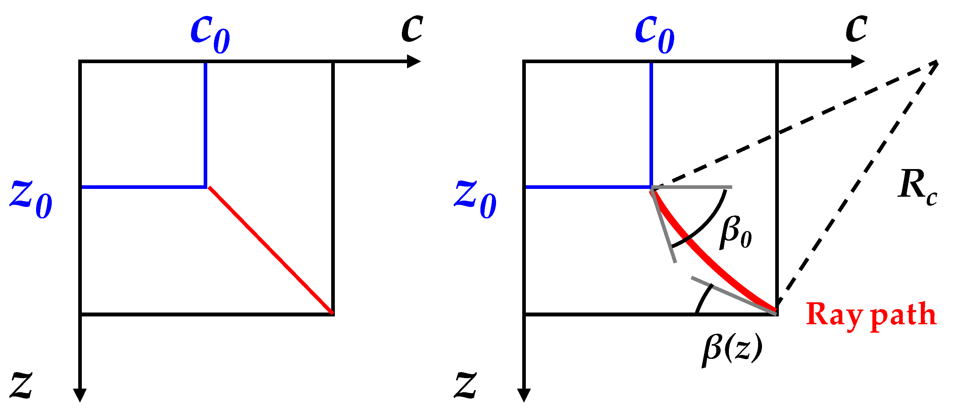
2.1. Theoretical Model of Ray Tracing

The development of predictive tools can also prove extremely useful in order to optimize the noise levels emitted at sea: the mathematical models are based on the phenomenological laws that govern the physics of wave propagation in fluids. The “Ray Tracing theory” represents a possible modeling approach for this purpose. This type of modeling is used in the optical field to analyze the light diffusion, but its applicability can also be extended to the acoustic field. This technique is a high-frequency approximation of the solution of the wave equation. It allows to define the propagation of sound through the emission of rays emitted by a point source in a medium at a constant speed of sound. The rays emitted by the source are perpendicular to the wave fronts, which are instead spherical surfaces radiated by the source itself. The reference theory is due to the Snell–Descartes law, which is used in acoustic geometry to describe the interference phenomena that occur between two homogeneous fluids having different speeds. Let us consider two fluids of which the first has density ρ1 and speed c1 and the second which has density ρ2 and speed c2 (with c2 > c1), as represented in Figure 1.
Snell–Descartes Theorem. The ratio of the cosines of the angles of incidence and refraction is equivalent to the ratio of phase velocities in the two media, or equivalent to the reciprocal of the ratio of the indices of refraction.
The difference in the velocity of the fluids means that the incident ray (inclined by the angle β1 with respect to the horizontal line) partially reflects upwards symmetrically and partially refracts in the second fluid with an angle β2 that is obtained from the following relationship (1):
c o s β 1 c 1 = c o s β 2 c 2
This equation is valid only if β2 ≤ 1 and therefore cosβ1c1/c2.
From this relation, it is possible to introduce another angle βcritic called “critical angle”, equal to Formula (2):
β c r i t i c = arccos ( c 1 c 2 )
For incidence angles β1 smaller than βcritic, there is total reflection. The same law can also be extended to study sound propagation phenomena when velocity varies linearly with depth.
Considering the law of variation of speed with depth as per Equation (3) (see Figure 2):
c ( z ) = c 0 + g ( z z 0 )
In which z is the vertical dimension and g is the speed gradient. Substituting the Equation (3) in the Snell–Descartes law Equation (1), the Equation (4) is obtained:
c o s β ( z ) = c ( z ) c 0 c o s β 0 = ( 1 + g c 0 ( z z 0 ) ) c o s β 0
Given the radius RC = c0/gcosβ0, the relationship (4) is reduced as follows:
c o s β ( z ) = c o s β 0 + z z 0 R C
It is observed, therefore, that in the case in which the speed varies with depth, the rays do not maintain straight trajectories but bend defining curved sections, unlike the case in which the speed remains constant and the rays propagate according to rectilinear sections. The method therefore consists in determining of the propagation of sound through linear segments and arcs that are connected along the water column, Figure 2. Relying upon this physical principle, the numerical prediction has been developed in this paper.

2.2. Numerical Prediction Code: Objectives and Functionality of the Program

The simulation program developed and described within this paper implements the basic foundations of this theory. The main purpose was to evaluate the Transmission Loss (TL) in water, and therefore the calculation of the sound pressure level (SPL) of a given point-like source that radiates a sound wave. The phases necessary to achieve this goal will be explained below, giving the reader the opportunity to get the program steps and then describing the applicative example about the noise analysis of the Adriatic Sea (Italy). From a general standpoint, the simulation code is structured in two distinct parts in order to guarantee greater speed and fluidity. The first part is dedicated to the input of the characteristic parameters of the source (the minimum angle, the maximum angle, and the step of emission of the rays) and of the surrounding environment (depth, temperature, salinity, pH). These data are fundamental to evaluate the water absorption coefficient α (Appendix A). Subsequently, the program, through a series of iterative cycles, will provide the different propagation paths of the rays emitted by the source. In the second part of the program, the user has the possibility to set up a matrix of virtual receivers through which to map the trend of the Transmission Loss (TL) and the SPL sound pressure level. The global layout is represented in Figure 3.

2.2.1. Propagation Paths

In evaluating the propagation paths, it was assumed that the velocity varies linearly with the depth through a law of this type (6):
c = c 1 + g 1 × z n
where c1 is the surface speed, g1 the speed gradient, and zn the various levels in which the water column is subdivided. The variation of the incident ray along the water column is evaluated as a function of the velocity along the different levels.
According to the Snell–Descartes law at each level:
-
If the angle of the i-th ray is greater than the critical angle, the latter will continue to propagate according to its direction until it reaches the bottom or the surface of the sea and then will reverse its direction.
-
If the angle of the i-th ray is greater than the critical angle, the latter will obviously reverse its direction of propagation before reaching the bottom.
Finally, one set of rays will reverse their direction when they interfere with the sea floor and surface while other rays will reverse their direction before reaching the bottom, tracing arch-shaped trajectories, Figure 4a. Once the different propagation paths have been obtained, the second part of the program requires the definition of the map of receivers such as to discretize the fluid domain, Figure 4b.

2.2.2. Calculation of the Loss of Propagation (TL)

When a wave propagates from a source, a reduction in intensity due both to the absorption of acoustic energy and to a loss of geometric diffusion (Appendix B) could be considered. Absorption was taken into account for the initial stage of the program, aiming to calculate the transmission loss ratio as follows in the Equation (7):
T L = 20 l o g R +   α R
In the case of rays incident on the sea floor, an absorption coefficient equal to 0.5 has been assumed, determining, therefore, an increase of 3 dB in the propagation loss according to Equation (8):
T L = 20 l o g R +   α R + 3 n
where n is the number of reflections on the sea floor.

2.2.3. Calculation of the Sound Pressure Level (SPL)

The SPL magnitude with respect to the acting pressure p is defined as the following quantity (9):
L P = 10 log 10 ( p p r e f ) 2     [ d B ]
in which pref represents the reference pressure evaluated at 1 m from the source and equal to 1 μPa. In order to evaluate the SPL due to the various sound fields, the linear sum of the pressures is automatically performed in Matab® (The MathWorks, Inc. Natick, MA, USA), assuming that:
( p i p r e f ) 2 = 10 S P L i / 10   [ P a ]
where pi is the i-th sound field pressure calculated at the receiver. The total sound field is obtained from the sum of the contributions of all pressures as per Equation (11):
S P L T O T = 10 log 10 ( i p i p r e f )     [ d B ]

2.3. Case Study Overview

As part of a collaboration between the University of Naples “Federico II” and Fincantieri technical department, the following program was developed to evaluate the propagation of sound in the Adriatic Sea, from a source located at a depth of 10 m from the sea surface. Five case studies were carried out in the same hydrogeological site, considering different depths with the purpose of making a final comparison of the different modes of transmission. The parameters used during the application and the expected results are outlined below.
  • SOURCE:
A point source located at –10m from the sea surface and with an SPL equal to 100 dB was assumed as a source of disturbance. With a range of rays varying between −90° and +90° with a step of 0.5°.
  • SEA AND CHARACTERISTICS:
The Adriatic Sea, as mentioned, was the reference marine environment for this research. This sea develops for a length of 800 km and a width of 200 km. This sea can be divided into three characteristic areas, Figure 5a:
-
A northern area characterized by a low percentage of salt due to the fact that the rivers flow into the basin. This area, which extends up to the cross of Ancona, is characterized by a shallow seabed.
-
A central area that goes from Ancona to the cross of the island of Pianosa, has a higher depth, and in particular, this area is characterized by warmer waters exhaled by the presence of the Ionian currents that penetrate through the Otranto Canal.
-
A southern area that extends along the coasts of Puglia where the maximum depth foreseen for this sea is reached, which is 1233 m in correspondence with the Gargano. This depression is also known as the “Fossa of the lower Adriatic”.
Based on this consideration, five case studies were elaborated by changing the depth of the seabed: from an average value of 250 m up to the maximum depth of 1250 m, with steps of 250 m assumed as the spatial range of investigation. So, the following cases were contemplated: 250 m, 500 m, 750 m, 1000 m, 1250 m. The characteristics of the sea are those reported in the MARCOAST (Marine and Coastal Environmental Information Services) project with which ISPRA (Higher Institute for Environmental Protection and Research) collaborated [42]. The project carried out a monitoring of the characteristics of the Adriatic Sea from 2007 to 2011. For the selection of the parameters, the average surface temperature measured in July 2008 (T = 24 °C) was considered, Figure 5b, while for the salinity, an average value based on ten-year surveys was chosen. The salinity chosen for the application is 37.62 psu (Practical Salinity Units), Figure 5c.
  • MATRIX OF RECEIVERS:
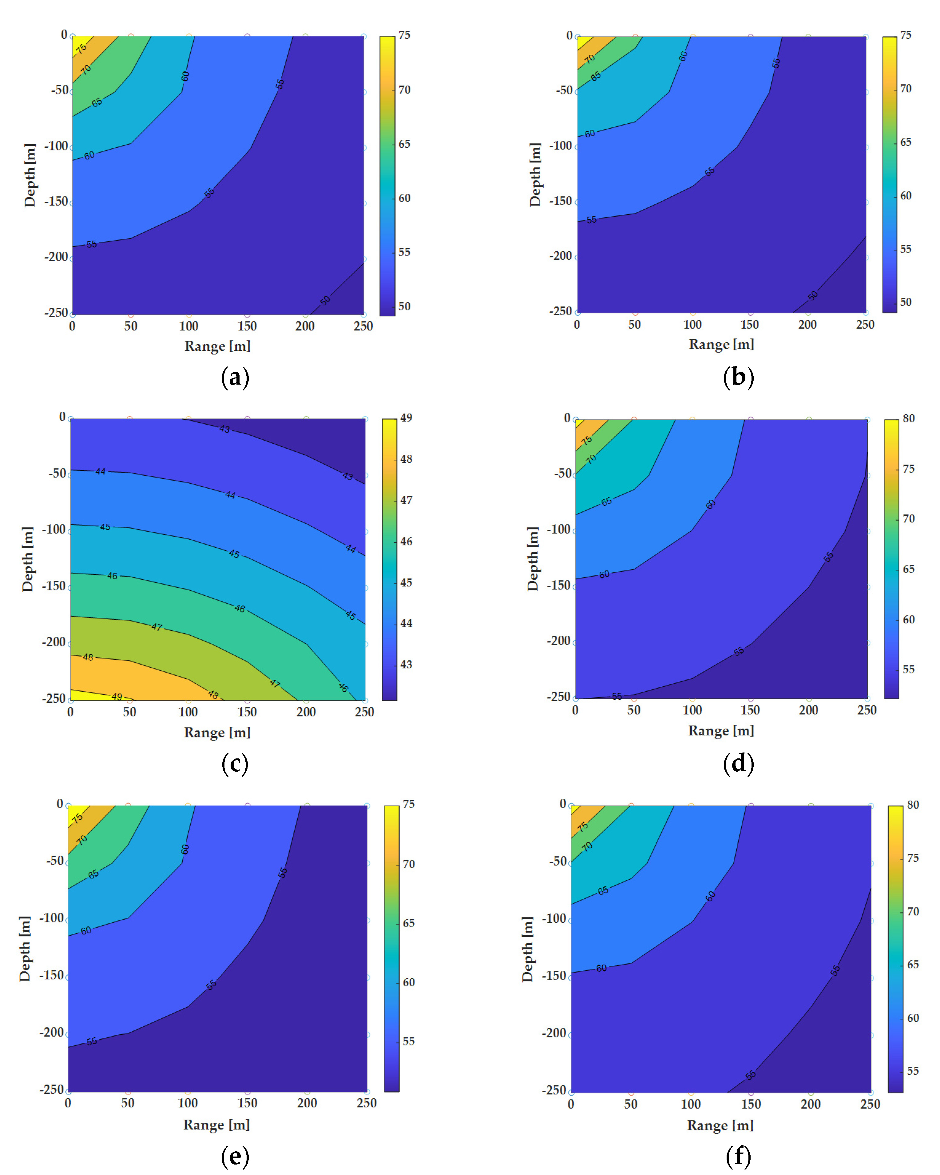
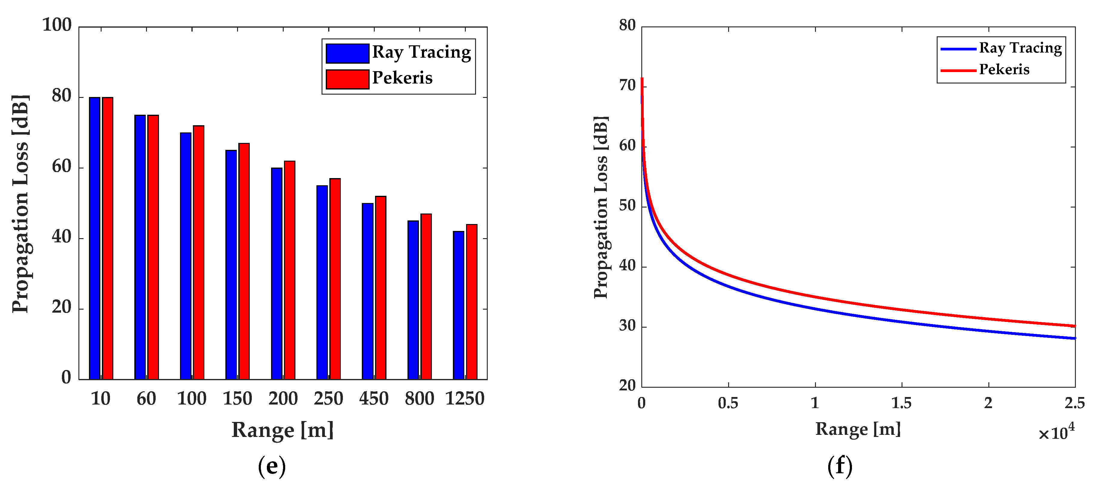
For the second part of the program, a matrix of 6 × 6 receivers distributed at intervals of equal width was set up as reported in Figure 4b.

3. Results

Following the logic of the previous paragraphs and exploiting the input data shown, the program will be able to graphically provide the different sound fields. At the end of processing, the program will graphically provide a series of sound fields. The first to be provided are: the direct sound field, the sound field after reflection on the free surface, the sound field after reflection on the seabed. Since sound can be composed, it is observed that the compound sound fields are obtained from the sum of direct and reflected sound fields. In fact, the program provides: the sound field composed between direct and reflected on the free surface, the sound field composed between direct and reflected on the bottom. Finally, the total one is obtained from the composition of the three sound fields, that is, total sound field composed of direct, reflected on the free surface, and reflected on the bottom. This reasoning was carried out for each case study and therefore at each depth. The simulations have been performed using an Intel® Core™ i7-6500U processor @2.50 GHz with 2 cores. These sound fields (direct, reflected, and combined) obtained for the particular case of maximum height of 250 m are represented in Figure 6. The composed acoustic contours representative of the other heights from the seabed, i.e., 500 m, 750 m, 1000 m, and 1250 m, are reported in Figure 7. The simulations show the importance of considering the reflected fields for the global propagation loss quantification. The global sound field in Figure 6f actually follows almost the same wave pattern as the direct field in Figure 6a but higher in amplitude: the resulting field reaches up to 55 dB against the 50 dB of the direct field only. As the coverage range increases, the SPL decays with a logarithmic law and as a function of the attenuation parameters illustrated above in paragraph 2: the acoustic level reaches a maximum of 40 dB at the distance of 1250 m, Figure 7d.

4. Discussion

In order to assess the Ray Tracing trend accuracy, the transmission loss has been compared with the Pekeris waveguide-based model; the purpose of such investigation was to deepen the basic understanding of the propagating mechanisms of underwater noise with respect to well-known theoretical schemes, especially for far-field cases. A maximum range of 25 km has been assumed. Below are the graphs representing a final comparison among the case studies, Figure 8.
The Pekeris model represents the simplest one to characterize shallow water acoustics, considering calm sea, constant depth, homogeneous medium non-absorbent seabed. The analyses showed an acceptable level of correlation between the Ray Tracing model, whose decay is a logarithmic function, and the transcended Pekeris model based instead on the propagation of normal modes; an average error of about 3 dB was estimated between the two approaches, which is acceptable in a preliminary design phase. For Pekeris, the rate of dispersion and waves attenuation in the waveguide depends on the iterative search of mode numbers. The wave equation is solved to determine the normal mode solutions which prevail at large distances from the source, according to Lamb procedure. For the present calculation, four normal modes have been supposed: the pressure field is calculated according to a two-dimensional modal extension (Kirchhoff equation). The discrepancy between two approaches could be found, therefore, in the different schematization of reflection and attenuation mechanisms, with the TL increasing with mode number [41]. Due to the broadband nature of the problem, the model is very computationally demanding. The calculation times essentially depend on the pitch of the rays and the distance to be covered. Performance can certainly be optimized by consolidating the simulation code structure. However, for a preliminary phase, these times are still advantageous with respect to finite element models, which required much more computational cost and mesh modeling steps as well. At the end of the processing, the time required for each simulation was evaluated: it is the function of two main parameters:
  • HEIGHT OF THE SEABED
The higher the height of the bottom, the more the processing time required for the simulation increases.
  • STEP BETWEEN RADIATION ANGLES
The code allows for inserting the interval between the emission rays of the source; the smaller the step, the more detailed the noise map will be. The computational cost varies quadratically with the depth of the sea, Figure 9. In Table 1, the times required by the program in the five cases.

5. Conclusions

This paper is part of the macro-topic inherent in the current need to study forecasting systems for optimizing the sources of underwater noise pollution generated by ship traffic. In particular, the activity arises from a collaboration between the University of Naples “Federico II” (industrial engineering department) and the technical office of Fincantieri Group with the purpose of creating a fast predictive code for a preliminary evaluation of the acoustic propagation fields in submarine environments, with special attention to the basin of the Adriatic Sea. The simulation program in Matlab® is essentially based on the optical-acoustic technique of Ray Tracing, which allows to characterize the sound propagation path also as a function of the characteristic parameters of the source and of the diffusion medium. Methodology is very suitable for preliminary calculations for two reasons:
  • For the identification of the sound field radiated even at a great distance and, therefore, of the impact this may have on the marine environment.
  • For the interpretation of the possible experimental values detected by the hydrophones in a field relatively close to the ship for an effective characterization of the disturbance source.
Future developments conducted by the research group aim at expanding the functionality of the program, taking into account also the third spatial dimension, while always limiting the computational cost, which, for applications of this kind, can be excessively expensive. Experimental campaigns of field measurements are also underway to validate this first part of the program.

Author Contributions

The authors (E.D., M.A., M.V., and T.C.) have equally contributed to this research paper. All authors have read and agreed to the published version of the manuscript.

Funding

This research received no external funding.

Conflicts of Interest

The authors declare no conflict of interest.

Appendix A

The theory used to evaluate the water absorption coefficient α is the model proposed by Francois–Garrison, in which the absorption coefficient is expressible into three terms that correspond, respectively, to the contribution of boric acid, of the sulphate of magnesium, and water viscosity:
α = A 1 P 1 f 1 f 2 f 1 2 + f 2 + A 2 P 2 f 2 f 2 f 2 2 + f 2 + A 3 P 3 f 2
  • Factors taking into account the contribution of boric acid B(OH)3:
    { A 1 = 8.86 c 10 0.78 p H S P 1 = 1     f 1 = 2.8 S 35 10 4 1245 T + 273 c = 1412 + 3.21 T + 1.19 S + 0.0167 z
  • Factors taking into account the contribution of magnesium sulfate Mg(SO)4:
    { A 2 = 21.44 S c ( 1 + 0.025 T ) P 2 = 1 1.37   × 10 4 z + 6.2   × 10 9 z 2 f 2 = 8.17   × 10 8 1990 T + 273 1 + 0.0018 ( S 35 )
  • Factors that take into account the contribution of water viscosity:
    P 3 = 1 3.83 × 10 5 z + 4.9   × 10 10 z 2 i f   T < 20 ° C A 3 = 4.937   × 10 4 2.59   × 10 5 T + 9.11   × 10 7 T 2 1.5 × 10 8 T 3 i f   T > 20 ° C f 2 = 8.17   × 10 8 1990 T + 273 1 + 0.0018 ( S 35 )

Appendix B

When a source emits a sound, it propagates in all directions in the form of surfaces whose sound levels are constant on each surface but decrease as the distance from the source increases. In fact, the sound wave propagating outwards causes a decrease in intensity proportional to the inverse of the surface. Near the source, the sound surfaces are spherical; as the radius increases, the diffusion will not always be spherical since there will be on one side the sea surface and on the other the seabed and, therefore, from a spherical diffusion, we pass to a cylindrical diffusion. For the two types of diffusion, the following (TL) transmission loss can be considered:
  • SPHERICAL DIFFUSION:
T L = 20 log ( R R 0 )
R0 is the reference level evaluated at 1 m from the source in a homogeneous non-dissipative medium
  • CYLINDRICAL DIFFUSION:
T L = 10 log ( r r 0 )
The transmission loss can be evaluated also taking into account the attenuation coefficient α . In this case, the relationship becomes:
T L = 20 l o g r + α r

References

  1. Knudsen, V.O.; Alford, R.S.; Emling, J.W. Underwater ambient noise. J. Mar. Res. 1948, 7, 410–429. [Google Scholar]
  2. Wenz, G.M. Acoustic ambient noise in the ocean: Spectra and sources. J. Acoust. Soc. Am. 1962, 34, 1936–1956. [Google Scholar] [CrossRef]
  3. Hildebrand, J.A. Anthropogenic and natural sources of ambient noise in the ocean. Mar. Ecol. Prog. Ser. 2009, 395, 5–20. [Google Scholar] [CrossRef] [Green Version]
  4. Committee on Potential Impacts of Ambient Noise in the Ocean on Marine Mammals. Ocean Noise and Marine Mammals; National Academies Press: Washington, DC, USA, 2003. [Google Scholar]
  5. Richardson, W.; Greene, C.; Malme, C.; Thomson, D. Marine Mammals and Noise; Academic Press: San Diego, CA, USA, 1995. [Google Scholar]
  6. Kozaczka, E.; Grelowska, G. Shipping low frequency noise and its propagation in shallow water. Acta Phys. Pol. A 2011, 119, 1009–1012. [Google Scholar] [CrossRef]
  7. Ross, D. Ship sources of ambient noise. IEEE J. Ocean. Eng. 2005, 30, 257–261. [Google Scholar] [CrossRef]
  8. Arveson, P.T.; Vendittis, D.T. Radiated noise characteristics of modern cargo ship. J. Acoust. Soc. Am. 2000, 107, 118–129. [Google Scholar] [CrossRef]
  9. Oceans and Law of the Sea (Division for Ocean Affairs and the Law of the Sea). United Nations Convention on the Law of the Sea. December 1982. Available online: www.un.org (accessed on 7 September 2020).
  10. Directive 2008/56/EC of the European Parliament and of the Council of 17 June 2008 Establishing a Framework for Community Action in the Field of Marine Environmental Policy (Marine Strategy Framework Directive). Available online: http://data.europa.eu/eli/dir/2008/56/oj (accessed on 7 September 2020).
  11. ISO 17208-2:2019. Underwater Acoustics—Quantities and Procedures for Description and Measurement of Underwater Sound from Ships. Available online: https://www.iso.org/standard/62409.html (accessed on 7 September 2020).
  12. International Towing Tank Conference (ITTC) Quality System Manual, Recommended Procedures and Guidelines, Underwater Noise from Ships, Full Scale Measurements. 2017. Available online: https://www.ittc.info/media/8183/75-04-04-01.pdf (accessed on 7 September 2020).
  13. International Maritime Organization (IMO). International Convention for the Prevention of Pollution from Ships (MARPOL); IMO: London, UK, 2 November 1973. [Google Scholar]
  14. Slabbekoorn, H.; Bouton, N.; van Opzeeland, I.; Coers, A.; ten Cate, C.; Popper, A.N. A noisy spring: The impact of globally rising underwater sound levels on fish. Trends Ecol. Evol. 2010, 25, 419–427. [Google Scholar] [CrossRef] [Green Version]
  15. Hawkins, A.; Pembroke, A.; Popper, A. Information gaps in understanding the effects of noise on fishes and invertebrates. Rev. Fish Biol. Fish. 2015, 25, 39–64. [Google Scholar] [CrossRef]
  16. Wright, A.J.; Highfill, L. Considerations of the effects of noise on marine mammals and other animals. Int. J. Comp. Psychol. 2007, 20, 89–316. [Google Scholar]
  17. Popper, A.; Hawkins, A.D. (Eds.) The Effects of Noise on Aquatic Life; Springer Science & Business Media: New York, NY, USA, 2012. [Google Scholar]
  18. Popper, A.; Hawkins, A.D. (Eds.) The Effects of Noise on Aquatic Life II. LLC; Springer Science + Business Media: New York, NY, USA, 2014. [Google Scholar]
  19. Popper, A.N.; Hastings, M.C. The effects of anthropogenic sources of sound on fishes. J. Fish Biol. 2009, 75, 455–489. [Google Scholar] [CrossRef]
  20. Erbe, C.; Marley, S.A.; Schoeman, R.P.; Smith, J.N.; Trigg, L.E.; Embling, C.B. The Effects of Ship Noise on Marine Mammals—A Review. Front. Mar. Sci. 2019, 6. [Google Scholar] [CrossRef] [Green Version]
  21. Southall, B.; Bowles, A.; Ellison, W.; Finneran, J.; Gentry, R.; Greene, C., Jr.; Kastak, D.; Ketten, D.; Miller, J.; Nachtigall, P. Marine mammal noise exposure criteria: Initial scientific recommendations. Aquat. Mamm. 2007, 33, 522. [Google Scholar]
  22. Rako-Gospić, N.; Picciulin, M. Underwater Noise: Sources and Effects on Marine Life. In World Seas: An Environmental Evaluation, 2nd ed.; Elsevier Academic Press: Amsterdam, The Netherlands, 2019; Volume III: Ecological Issues and Environmental Impacts, Chapter 20; pp. 367–389. [Google Scholar]
  23. McDonald, M.A.; Hildebrand, J.A.; Wiggins, S.M.; Ross, D. A 50 year comparison of ambient ocean noise near San Clemente Island: A bathymetrically complex coastal region off Southern California. J. Acoust. Soc. Am. 2008, 124, 1985–1992. [Google Scholar] [CrossRef] [PubMed]
  24. Wagstaff, R.A. Low-frequency ambient noise in the deep sound channel—The missing component. J. Acoust. Soc. Am. 1981, 69, 1009–1014. [Google Scholar] [CrossRef]
  25. Bannister, R.W. Deep sound channel noise from high latitude winds. J. Acoust. Soc. Am. 1986, 79, 41–48. [Google Scholar] [CrossRef]
  26. Andrew, R.; Howe, B.; Mercer, J.; Dziecuich, M. Ocean ambient sound: Comparing the 1960’s with the 1990’s for a receiver off the California coast. Acoust. Res. Lett. Online 2002, 3, 65–70. [Google Scholar] [CrossRef] [Green Version]
  27. McDonald, M.A.; Hildebrand, J.A.; Wiggins, S.M. Increases in deep-ocean ambient noise in the Northeast Pacific west of San Nicholas Island, California. J. Acoust. Soc. Am. 2006, 120, 711–718. [Google Scholar] [CrossRef] [Green Version]
  28. Carey, W.B.; Evans, R.B. Ocean Ambient Noise, Measurement and Theory; Springer: New York, NY, USA, 2011; p. 263. [Google Scholar]
  29. Kozaczka, E.; Grelowska, G. Shipping noise. Arch. Acoust. 2004, 29, 169–176. [Google Scholar]
  30. Kozaczka, E. Investigations of underwater disturbances generated by the ship propeller. Arch. Acoust. 1978, 13, 133–152. [Google Scholar]
  31. Ross, D. Mechanics of Underwater Noise; Pergamon: New York, NY, USA, 1976. [Google Scholar]
  32. Kozaczka, E.; Domagalski, J.; Grelowska, G.; Gloza, I. Identification of hydroacoustic waves emitted from floating units during mooring tests. Pol. Marit. Res. 2007, 14, 40–46. [Google Scholar] [CrossRef] [Green Version]
  33. Kozaczka, E.; Grelowska, G.; Gloza, I. Sound Intensity in Ships Noise Measuring. In Proceedings of the 19th International Congress on Acoustics (ICA), 6 pp. CD, Madrid, Spain, 2–7 September 2007. [Google Scholar]
  34. Grelowska, G.; Kozaczka, E.; Kozaczka, S.; Szymczak, W. Some Aspects of Noise Generated by a Small Ship in the Shallow Sea. In Proceedings of the 11th European Conference on Underwater Acoustics, Edinburgh, UK, 2–6 July 2012. [Google Scholar]
  35. Urick, R.J. Principles of Underwater Sound; Mc Graw-Hill: New York, NY, USA, 1975; Chapter 10. [Google Scholar]
  36. Grelowska, G.; Kozaczka, E.; Kozaczka, S.; Szymczak, W. Underwater Noise Generated by a Small Ship in the Shallow Sea. Arch. Acoust. 2013, 38, 351–356. [Google Scholar] [CrossRef]
  37. McKenna, M.F.; Ross, D.; Wiggins, D.M. Underwater radiated noise from modern commercial ships. J. Acoust. Soc. Am. 2012, 131, 92–103. [Google Scholar] [CrossRef] [PubMed] [Green Version]
  38. Trevorrow, M.V.; Vasiliev, B.; Vagle, S. Directionality and maneuvering effects on a surface ship underwater acoustic signature. J. Acoust. Soc. Am. 2008, 124, 767–778. [Google Scholar] [CrossRef] [PubMed] [Green Version]
  39. Gloza, I. Experimental Investigation of Underwater Noise Produced by Ships by Means of Sound Intensity Method. Acta Phys. Pol. A 2010, 118, 58–61. [Google Scholar] [CrossRef]
  40. Zhang, G.; Forland, T.N.; Johnsen, E.; Pedersen, G.; Dong, H. Measurements of underwater noise radiated by commercial ships at a cabled ocean observatory. Mar. Pollut. Bull. 2020, 153, 110948. [Google Scholar] [CrossRef]
  41. Pekeris, C.L. Theory of Propagation of Explosive Sound in Shallow Water. Book Chapter. In Propagation of Sound in the Ocean; Geological Society of America Geological Society of America: Boulder, CO, USA, 1 January 1948. [Google Scholar] [CrossRef]
  42. Ceriola, G.; Viel, M.; Silvestri, C.; Campbell, G. MarCoast, Servizi di Qualità delle Acque da dati satellitari per mari europei. In Proceedings of the 13th National Conference ASITA (Italian Federation of Scientific Associations), Bari, Italy, 1–4 December 2009. [Google Scholar]
  43. The Adriatic forecasting system. Available online: http://oceanlab.cmcc.it/aifs/ (accessed on 7 September 2020).
  44. Meteorological and Hydrological Service. Available online: https://meteo.hr/index_en.php (accessed on 7 September 2020).
  45. Bas, A.A.; Affinito, F.; Martin, S.; Vollmer, A.; Gansen, C.; Morris, N.; Frontier, N.; Nikpaljevic, N.; Vujović, A. Bottlenose Dolphins and Striped dolphins: Species Distribution, Behavioural Patterns, Encounter Rates, Residency Patterns and Hotspots in Montenegro, South Adriatic (2016–2017); Annual Report, Montenegro Dolphin Project; DMAD: Antalya, Turkey, 2018. [Google Scholar]
Figure 1. Incident ray which partly reflects and partly is transmitted in the second fluid.
Fluids 06 00019 g001
Figure 2. Trend of the rays when the speed varies linearly with the depth.
Fluids 06 00019 g002
Figure 3. Logical schematic of the numerical code.
Fluids 06 00019 g003
Figure 4. Simulation setup: (a) rays of propagation; (b) receiver matrix.
Fluids 06 00019 g004
Figure 5. Characterization maps of the Adriatic Sea: (a) depth map, [43,44,45]; (b) water temperature distribution (c) water salinity distribution.
Fluids 06 00019 g005
Figure 6. Acoustic field propagation at 250 m: (a) direct sound field; (b) reflection on the free side; (c) reflection on the sea floor; (d) direct and reflected field on the free side combination; (e) direct and reflected on the sea floor combination; (f) global sound field.
Fluids 06 00019 g006
Figure 7. Global acoustic field at different heights: (a) z = 500 m; (b) z = 750 m; (c) z = 1000 m; (d) z = 1250 m.
Fluids 06 00019 g007aFluids 06 00019 g007b
Figure 8. Trend of the propagation loss at different conditions compared with the Pekeris model predictions: (a) 250 m; (b) 500 m; (c) 750 m; (d) 1000 m; (e) 1250 m; (f) range up to 25 km.
Fluids 06 00019 g008aFluids 06 00019 g008b
Figure 9. CPU time estimation as function of sea depth.
Fluids 06 00019 g009
Table 1. Computational cost estimation as function of sea depth.
SIMULATIONSDEPTHTIME REQUIRED
CASE I250 m9.86 min
CASE II500 m30.47 min
CASE III750 m55.30 min
CASE IV1000 m92.05 min
CASE V1250 m137.54 min
Publisher’s Note: MDPI stays neutral with regard to jurisdictional claims in published maps and institutional affiliations.

