Experimental Data for the Validation of Numerical Methods: DrivAer Model


Abstract
1. Introduction
2. Experimental Methodology
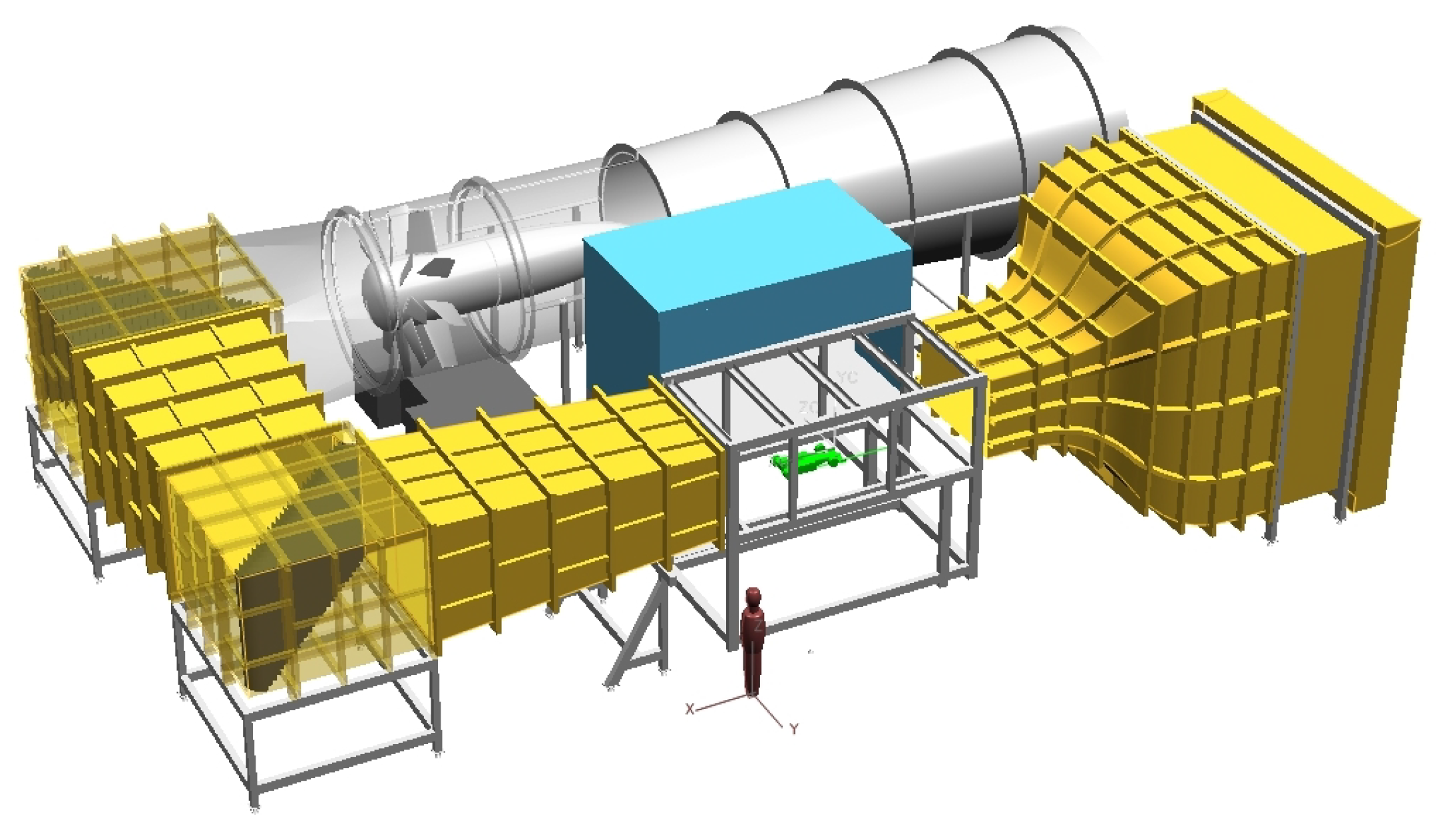
2.1. Facilities
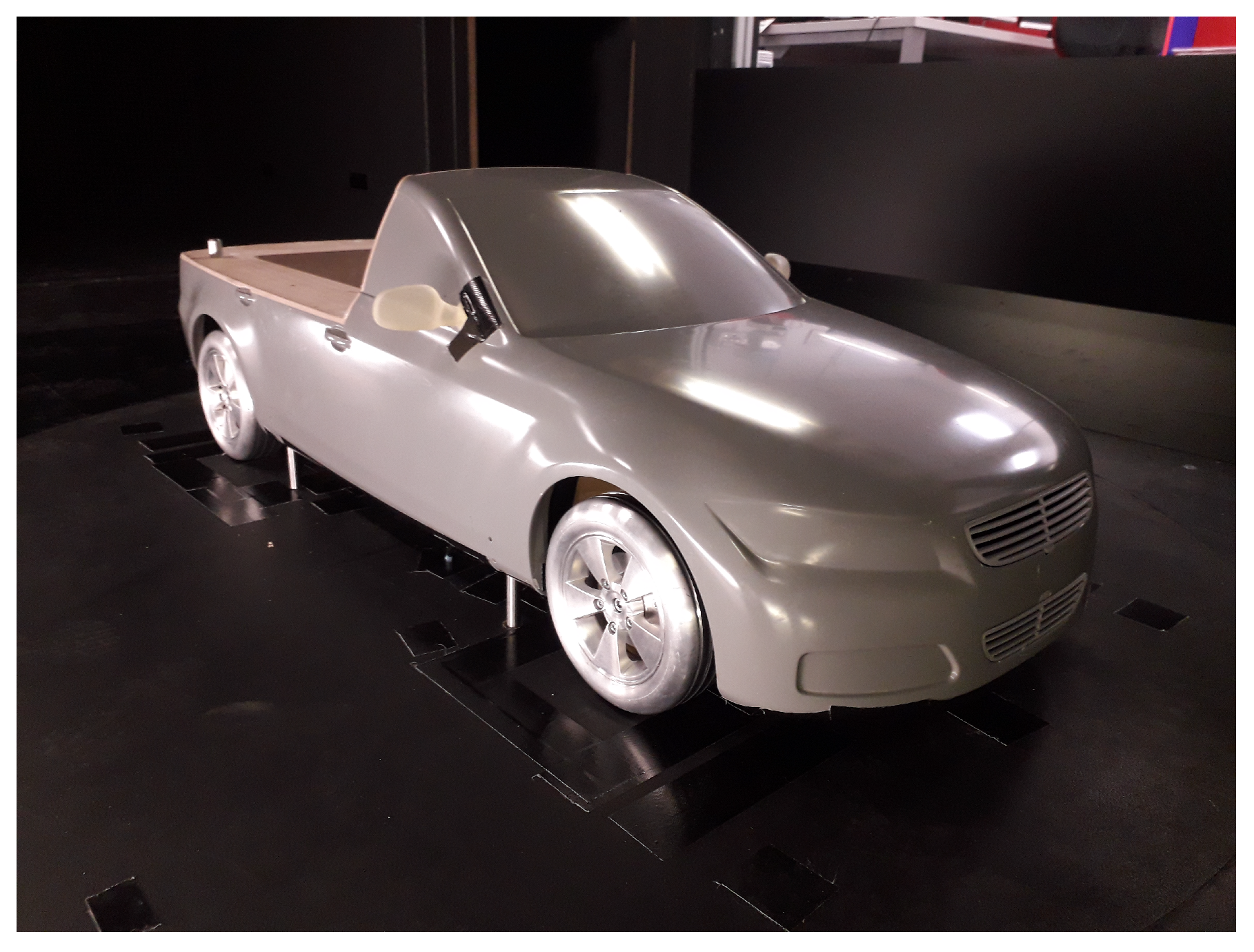
2.2. Model
2.3. Measurements
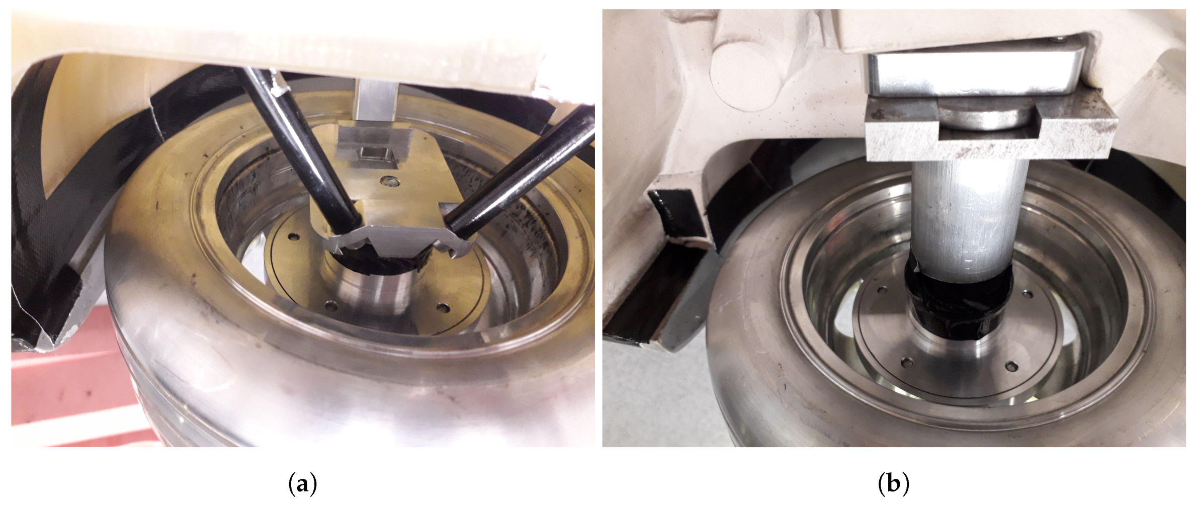
2.3.1. Force
2.3.2. Pressures
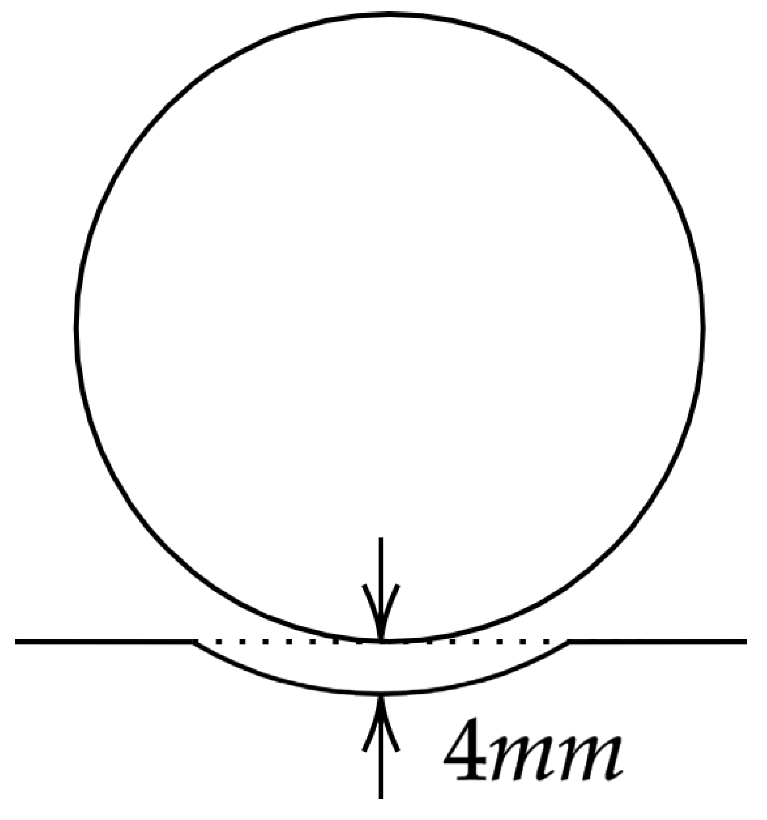
2.3.3. Velocity Field
3. Results
4. Conclusions
Author Contributions
Funding
Acknowledgments
Conflicts of Interest
Appendix A. Previous Literature Results

| Body | Wheels | Underbody | Cooling Flow | Mirrors | Tunnel | Scale (%) | Blockage (%) | Reynolds Number () | Ground Simulation | Citation | ||
|---|---|---|---|---|---|---|---|---|---|---|---|---|
| Estate | Static | Smooth | N | Y | 1.4MW—Monash | 100 | 20.7 | 8 | Static | 0.291 | - | [41] |
| Estate | Proprietry | Smooth | N | Y | AAWK—Audi | 40 | 3.15 | 5.2 | 1 Belt | 0.298 | −0.007 | [35] |
| Fast | Proprietry | Smooth | N | Y | AAWK—Audi | 40 | 3.15 | 5.2 | 1 Belt | 0.251 | 0.024 | [35] |
| Notch | Proprietry | Smooth | N | Y | AAWK—Audi | 40 | 3.15 | 5.2 | 1 Belt | 0.255 | 0.004 | [35] |
| Estate | Proprietry | Smooth | N | Y | WTA—TU Munich | 40 | 8 | 5.2 | 1 Belt | 0.299 | −0.154 | [35] |
| Fast | Proprietry | Smooth | N | Y | WTA—TU Munich | 40 | 8 | 5.2 | 1 Belt | 0.252 | −0.008 | [35] |
| Notch | Proprietry | Smooth | N | Y | WTA—TU Munich | 40 | 8 | 5.2 | 1 Belt | 0.255 | −0.028 | [35,58] |
| Fast | Proprietry | Detailed | N | Y | WTA—TU Munich | 40 | 8.3 | 4.9 | 1 Belt | 0.275 | - | [8] |
| Fast | Proprietry | Detailed | N | N | WTA—TU Munich | 40 | 8.3 | 4.9 | 1 Belt | 0.261 | - | [8] |
| Notch | Proprietry | Detailed | N | Y | WTA—TU Munich | 40 | 8.3 | 4.9 | 1 Belt | 0.277 | - | [8] |
| Notch | Proprietry | Detailed | N | N | WTA—TU Munich | 40 | 8.3 | 4.9 | 1 Belt | 0.262 | - | [8] |
| Estate | Proprietry | Detailed | N | Y | WTA—TU Munich | 40 | 8.3 | 4.9 | 1 Belt | 0.319 | - | [8] |
| Estate | Proprietry | Detailed | N | N | WTA—TU Munich | 40 | 8.3 | 4.9 | 1 Belt | 0.307 | - | [8] |
| Fast | Proprietry | Smooth | N | Y | WTA—TU Munich | 40 | 8.3 | 4.9 | 1 Belt | 0.243 | - | [8] |
| Fast | Proprietry | Smooth | N | N | WTA—TU Munich | 40 | 8.3 | 4.9 | 1 Belt | 0.227 | - | [8] |
| Notch | Proprietry | Smooth | N | Y | WTA—TU Munich | 40 | 8.3 | 4.9 | 1 Belt | 0.246 | - | [8] |
| Notch | Proprietry | Smooth | N | N | WTA—TU Munich | 40 | 8.3 | 4.9 | 1 Belt | 0.232 | - | [8] |
| Estate | Proprietry | Smooth | N | Y | WTA—TU Munich | 40 | 8.3 | 4.9 | 1 Belt | 0.292 | - | [8] |
| Estate | Proprietry | Smooth | N | N | WTA—TU Munich | 40 | 8.3 | 4.9 | 1 Belt | 0.28 | - | [8] |
| Fast | Proprietry | Detailed | N | Y | WTA—TU Munich | 40 | 8.3 | 4.9 | Static | 0.284 | - | [8] |
| Fast | Proprietry | Detailed | N | N | WTA—TU Munich | 40 | 8.3 | 4.9 | Static | 0.269 | - | [8] |
| Notch | Proprietry | Detailed | N | Y | WTA—TU Munich | 40 | 8.3 | 4.9 | Static | 0.286 | - | [8] |
| Notch | Proprietry | Detailed | N | N | WTA—TU Munich | 40 | 8.3 | 4.9 | Static | 0.271 | - | [8] |
| Estate | Proprietry | Detailed | N | Y | WTA—TU Munich | 40 | 8.3 | 4.9 | Static | 0.319 | - | [8] |
| Estate | Proprietry | Detailed | N | N | WTA—TU Munich | 40 | 8.3 | 4.9 | Static | 0.306 | - | [8] |
| Fast | Proprietry | Smooth | N | Y | WTA—TU Munich | 40 | 8.3 | 4.9 | Static | 0.254 | - | [8] |
| Fast | Proprietry | Smooth | N | N | WTA—TU Munich | 40 | 8.3 | 4.9 | Static | 0.242 | - | [8] |
| Notch | Proprietry | Smooth | N | Y | WTA—TU Munich | 40 | 8.3 | 4.9 | Static | 0.258 | - | [8] |
| Notch | Proprietry | Smooth | N | N | WTA—TU Munich | 40 | 8.3 | 4.9 | Static | 0.243 | - | [8] |
| Estate | Proprietry | Smooth | N | Y | WTA—TU Munich | 40 | 8.3 | 4.9 | Static | 0.296 | - | [8] |
| Estate | Proprietry | Smooth | N | N | WTA—TU Munich | 40 | 8.3 | 4.9 | Static | 0.283 | - | [8] |
| Notch | Static | Detailed | N | N | AWT—Ford | 100 | 10.6 | 11.8 | Static | 0.259 | 0.112 | [32] |
| Fast | Static | Detailed | N | N | AWT—Ford | 100 | 10.6 | 11.8 | Static | 0.260 | 0.130 | [32] |
| Estate | Static | Detailed | N | N | AWT—Ford | 100 | 10.6 | 11.8 | Static | 0.291 | −0.015 | [32] |
| Notch | Static | Detailed | N | N | AWT—Ford | 100 | 10.6 | ≈ | Static | 0.261 | - | [32] |
| Notch | Static | Detailed | N | N | AWT—Ford | 100 | 10.6 | ≈ | Static | 0.263 | - | [32] |
| Notch | Static | Smooth | N | N | AWT—Ford | 100 | 10.6 | 11.8 | Static | 0.233 | 0.051 | [32] |
| Fast | Static | Smooth | N | N | AWT—Ford | 100 | 10.6 | 11.8 | Static | 0.230 | 0.051 | [32] |
| Estate | Static | Smooth | N | N | AWT—Ford | 100 | 10.6 | 11.8 | Static | 0.273 | −0.087 | [32] |
| Notch | Static | Detailed | N | N | DTF—Ford | 100 | 11.3 | ≈ | Static | 0.264 | - | [32] |
| Notch | Static | Detailed | N | N | DTF—Ford | 100 | 11.3 | 11.8 | Static | 0.258 | - | [32] |
| Notch | Static | Detailed | N | N | DTF—Ford | 100 | 11.3 | ≈ | Static | 0.261 | - | [32] |
| Notch | Static | Detailed | N | N | 1.4 MW—Monash | 100 | 16.1 | ≈ | Static | 0.254 | - | [32] |
| Notch | Static | Detailed | N | N | 1.4 MW—Monash | 100 | 16.1 | 11.8 | Static | 0.253 | ≈ | [32] |
| Notch | Yes | Detailed | N | N | Tongji | 100 | 7.9 | ≈ | 5 Belt | 0.253 | - | [32] |
| Notch | Yes | Detailed | N | N | Tongji | 100 | 7.9 | 11.8 | 5 Belt | 0.244 | ≈ | [32] |
| Notch | Yes | Detailed | N | N | Tongji | 100 | 7.9 | ≈ | 5 Belt | 0.24 | - | [32] |
| Notch | Static | Detailed | N | N | Tongji | 100 | 7.9 | ≈ | Static | 0.263 | - | [32] |
| Notch | Static | Detailed | N | N | Tongji | 100 | 7.9 | 11.8 | Static | 0.265 | ≈ | [32] |
| Notch | Static | Detailed | N | N | Tongji | 100 | 7.9 | ≈ | Static | 0.265 | - | [32] |
| Notch | Yes | Detailed | N | N | PVT—Volvo | 100 | 7.8 | ≈ | 5 Belt | 0.26 | - | [32] |
| Notch | Yes | Detailed | N | N | PVT—Volvo | 100 | 7.8 | 11.8 | 5 Belt | 0.254 | ≈ | [32] |
| Notch | Yes | Detailed | N | N | PVT—Volvo | 100 | 7.8 | ≈ | 5 Belt | 0.248 | - | [32] |
| Notch | Static | Detailed | N | N | PVT—Volvo | 100 | 7.8 | ≈ | Static | 0.276 | - | [32] |
| Notch | Static | Detailed | N | N | PVT—Volvo | 100 | 7.8 | 11.8 | Static | 0.277 | ≈ | [32] |
| Notch | Static | Detailed | N | N | PVT—Volvo | 100 | 7.8 | ≈ | Static | 0.278 | - | [32] |
| Notch | Yes | Detailed | N | N | Windshear Inc. | 100 | 12.7 | ≈ | 1 Belt | 0.247 | - | [32] |
| Notch | Yes | Detailed | N | N | Windshear Inc. | 100 | 12.7 | 11.8 | 1 Belt | 0.242 | ≈ | [32] |
| Notch | Yes | Detailed | N | N | Windshear Inc. | 100 | 12.7 | ≈ | 1 Belt | 0.24 | - | [32] |
| Notch | Static | Detailed | N | N | Windshear Inc. | 100 | 12.7 | ≈ | Static | 0.259 | - | [32] |
| Notch | Static | Detailed | N | N | Windshear Inc. | 100 | 12.7 | 11.8 | Static | 0.271 | ≈ | [32] |
| Notch | Static | Detailed | N | N | Windshear Inc. | 100 | 12.7 | ≈ | Static | 0.274 | - | [32] |
| Notch | Yes | Detailed | N | Y | MWK—FKFS | 25 | - | 3.8 | 5 Belt | 0.282 | 0.073 | [42] |
| Estate | Yes | Detailed | N | Y | MWK—FKFS | 25 | - | 3.8 | 5 Belt | 0.309 | −0.041 | [42] |
| Fast | Yes | Detailed | N | Y | MWK—FKFS | 25 | - | 3.8 | 5 Belt | 0.28 | 0.09 | [42] |
| Notch | Yes | Detailed | Y | Y | MWK—FKFS | 25 | - | 3.8 | 5 Belt | 0.289 | 0.074 | [42] |
| Notch | Yes | Smooth | N | Y | MWK—FKFS | 25 | - | 3.8 | 5 Belt | 0.261 | 0.041 | [42] |
| Fast | Proprietry | Detailed | N | Y | WTA—TU Munich | 40 | 8.3 | 5.2 | 1 Belt | 0.274 | - | [7] |
| Notch | Proprietry | Detailed | N | Y | WTA—TU Munich | 40 | 8.3 | 5.2 | 1 Belt | 0.275 | - | [7] |
| Estate | Proprietry | Detailed | N | Y | WTA—TU Munich | 40 | 8.3 | 5.2 | 1 Belt | 0.314 | - | [7] |
| Fast | Proprietry | Generic | N | Y | WTA—TU Munich | 40 | 8.3 | 5.2 | 1 Belt | 0.253 | - | [7] |
| Notch | Proprietry | Generic | N | Y | WTA—TU Munich | 40 | 8.3 | 5.2 | 1 Belt | 0.257 | - | [7] |
| Estate | Proprietry | Generic | N | Y | WTA—TU Munich | 40 | 8.3 | 5.2 | 1 Belt | 0.302 | - | [7] |
| Fast | Proprietry | Smooth | N | N | WTA—TU Munich | 40 | 8.3 | 5.2 | 1 Belt | 0.228 | - | [7] |
| Notch | Proprietry | Smooth | N | N | WTA—TU Munich | 40 | 8.3 | 5.2 | 1 Belt | 0.233 | - | [7] |
| Estate | Proprietry | Smooth | N | N | WTA—TU Munich | 40 | 8.3 | 5.2 | 1 Belt | 0.28 | - | [7] |
| Fast | Proprietry | Smooth | N | Y | WTA—TU Munich | 40 | 8.3 | 5.2 | 1 Belt | 0.247 | - | [7] |
| Notch | Proprietry | Smooth | N | Y | WTA—TU Munich | 40 | 8.3 | 5.2 | 1 Belt | 0.252 | - | [7] |
| Estate | Proprietry | Smooth | N | Y | WTA—TU Munich | 40 | 8.3 | 5.2 | 1 Belt | 0.296 | - | [7] |
| Fast | Proprietry | Detailed | N | Y | WTA—TU Munich | 40 | 8.3 | 5.2 | Static | 0.272 | - | [7] |
| Notch | Proprietry | Detailed | N | Y | WTA—TU Munich | 40 | 8.3 | 5.2 | Static | 0.272 | - | [7] |
| Estate | Proprietry | Detailed | N | Y | WTA—TU Munich | 40 | 8.3 | 5.2 | Static | 0.303 | - | [7] |
| Fast | Proprietry | Generic | N | Y | WTA—TU Munich | 40 | 8.3 | 5.2 | Static | 0.257 | - | [7] |
| Notch | Proprietry | Generic | N | Y | WTA—TU Munich | 40 | 8.3 | 5.2 | Static | 0.257 | - | [7] |
| Estate | Proprietry | Generic | N | Y | WTA—TU Munich | 40 | 8.3 | 5.2 | Static | 0.292 | - | [7] |
| Fast | Proprietry | Smooth | N | N | WTA—TU Munich | 40 | 8.3 | 5.2 | Static | 0.238 | - | [7] |
| Notch | Proprietry | Smooth | N | N | WTA—TU Munich | 40 | 8.3 | 5.2 | Static | 0.24 | - | [7] |
| Estate | Proprietry | Smooth | N | N | WTA—TU Munich | 40 | 8.3 | 5.2 | Static | 0.278 | - | [7] |
| Fast | Proprietry | Smooth | N | Y | WTA—TU Munich | 40 | 8.3 | 5.2 | Static | 0.249 | - | [7] |
| Notch | Proprietry | Smooth | N | Y | WTA—TU Munich | 40 | 8.3 | 5.2 | Static | 0.251 | - | [7] |
| Estate | Proprietry | Smooth | N | Y | WTA—TU Munich | 40 | 8.3 | 5.2 | Static | 0.286 | - | [7] |
| Fast | No | Smooth | N | N | WTA—TU Munich | 40 | 8.3 | 5.2 | 1 Belt | 0.117 | −0.345 | [7,33] |
| Notch | No | Smooth | N | N | WTA—TU Munich | 40 | 8.3 | 5.2 | 1 Belt | 0.129 | −0.37 | [7,33] |
| Estate | No | Smooth | N | N | WTA—TU Munich | 40 | 8.3 | 5.2 | 1 Belt | 0.192 | −0.494 | [7,33] |
| Fast | No | Smooth | N | N | WTA—TU Munich | 40 | 8.3 | 5.2 | Static | 0.116 | −0.295 | [7,33] |
| Notch | No | Smooth | N | N | WTA—TU Munich | 40 | 8.3 | 5.2 | Static | 0.127 | −0.319 | [7,33] |
| Estate | No | Smooth | N | N | WTA—TU Munich | 40 | 8.3 | 5.2 | Static | 0.19 | −0.446 | [7,33] |
| Fast | Proprietry | Smooth | N | N | WTA—TU Munich | 40 | 8.3 | 5.2 | 1 Belt | 0.244 | −0.031 | [33] |
| Notch | Proprietry | Smooth | N | N | WTA—TU Munich | 40 | 8.3 | 5.2 | 1 Belt | 0.247 | −0.014 | [33] |
| Estate | Proprietry | Smooth | N | N | WTA—TU Munich | 40 | 8.3 | 5.2 | 1 Belt | 0.291 | −0.146 | [33] |
| Fast | Proprietry | Smooth | N | N | WTA—TU Munich | 40 | 8.3 | 5.2 | Static | 0.245 | −0.003 | [33] |
| Notch | Proprietry | Smooth | N | N | WTA—TU Munich | 40 | 8.3 | 5.2 | Static | 0.246 | 0.002 | [33] |
| Estate | Proprietry | Smooth | N | N | WTA—TU Munich | 40 | 8.3 | 5.2 | Static | 0.282 | −0.123 | [33] |
| Fast | No | Smooth | N | Y | 8x6WT—Cranfield | 35 | 10.2 | 2.1-4.2 | 1 Belt | ≈ | −0.75 −−0.84 | [46] |
| Notch | Static | Detailed | N | Y | MWK—FKFS | 25 | - | 3.2 | Static | 0.278 | - | [37] |
| Estate | Static | Detailed | N | Y | MWK—FKFS | 25 | - | 3.2 | Static | 0.303 | - | [37] |
| Fast | Static | Smooth | N | Y | MWK—TU Berlin | 25 | 5.5 | 2.8 | False floor | 0.249 | 0.057 | [38] |
| Fast | Static | Smooth | N | Y | MWK—TU Berlin | 25 | 5.4 | 3.2 | False floor | 0.258 | −0.096 | [39] |
| Notch | Static | Smooth | N | Y | MWK—TU Berlin | 25 | 5.4 | 3.2 | False floor | 0.254 | −0.107 | [39] |
| Notch | Static | Smooth | N | Y | MWK—TU Berlin | 25 | 5.4 | 3 | False floor | - | - | [40] |
| Notch | Yes | Detailed | N | Y | MWK—FKFS | 25 | - | 4.6 | 5 Belt | 0.277 | 0.059 | [34] |
| Estate | Yes | Detailed | N | Y | MWK—FKFS | 25 | - | 4.6 | 5 Belt | 0.312 | −0.059 | [34] |
| Notch | Yes | Detailed | Y | Y | MWK—FKFS | 25 | - | 4.6 | 5 Belt | 0.284 | ≈0.055 | [34] |
| Estate | Yes | Detailed | Y | Y | MWK—FKFS | 25 | - | 4.6 | 5 Belt | 0.322 | ≈−0.055 | [34] |
Appendix B. Dataset README File (V1.0)
References
- Wood, D.; Passmore, M.A.; Perry, A.K. Experimental Data for the Validation of Numerical Methods - SAE Reference Notchback Model. SAE Int. J. Passeng. Cars Mech. Syst. 2014, 7, 145–154. [Google Scholar] [CrossRef]
- Nader, A.; Islam, A.; Thornber, B. A Comparative Aerodynamic Investigation of a 20∘ SAE Notchback Model. Appl. Mech. Mater. 2016, 846, 79–84. [Google Scholar] [CrossRef]
- Törnell, J. PANS Prediction of Passenger Vehicle Flows. Master’s Thesis, Chalmers University of Technology, Göteborg, Sweden, 2016. [Google Scholar]
- Islam, A.; Thornber, B. Development and Application of a novel RANS and Implicit les Hybrid Turbulence Model for Automotive Aerodynamics. SAE Technol. Pap. 2016. [Google Scholar] [CrossRef]
- Islam, A.; Thornber, B. High-order detached-eddy simulation of external aerodynamics over an SAE notchback model. Aeronaut. J. 2017, 121, 1342–1367. [Google Scholar] [CrossRef]
- Varney, M.; Passmore, M.; Wittmeier, F.; Kuthada, T. DrivAer Experimental Aerodynamic Dataset, 2020. Available online: https://repository.lboro.ac.uk/articles/dataset/DrivAer_Experimental_Aerodynamic_Dataset/12881213 (accessed on 1 October 2020).
- Mack, S.; Indinger, T.; Adams, N.A.; Blume, S.; Unterlechner, P. The Interior Design of A 40 Scaled Drivaer Body and First Experimental Results. In Proceedings of the ASME 2012 Fluids Engineering Division SummerMeeting, American Society of Mechanical Engineers, Rio Grande, PR, USA, 8–12 July 2012. [Google Scholar]
- Heft, A.I.; Indinger, T.; Adams, N.A. Introduction of a new realistic generic car model for aerodynamic investigations. SAE Technol. Pap. 2012. [Google Scholar] [CrossRef]
- Ashton, N.; Revell, A. Comparison of RANS and des methods for the DrivAer automotive body. SAE Technol. Pap. 2015. [Google Scholar] [CrossRef]
- Jakirlic, S.; Kutej, L.; Hanssmann, D.; Basara, B.; Tropea, C. Eddy-resolving Simulations of the Notchback ’DrivAer’ Model: Influence of Underbody Geometry and Wheels Rotation on Aerodynamic Behaviour. SAE Technol. Pap. 2016. [Google Scholar] [CrossRef]
- Howell, J.; Forbes, D.; Passmore, M.; Page, G. The Effect of a Sheared Crosswind Flow on Car Aerodynamics. SAE Int. J. Passeng. Cars Mech. Syst. 2017, 10. [Google Scholar] [CrossRef]
- Jungmann, J.; Schütz, T.; Jakirlic, S.; Tropea, C. Flow past a DrivAer body in a scaled wind tunnel: Computational study by a reference to a complementary experiment. In Proceedings of the IMechE International Conference on Vehicle Aerodynamics, Coventry, UK, 21–22 September 2016. [Google Scholar]
- Peters, B.C.; Uddin, M.; Bain, J.; Curley, A.; Henry, M. Simulating DrivAer with Structured Finite Difference Overset Grids. SAE Technol. Pap. 2015. [Google Scholar] [CrossRef]
- Fields, V.; E-mail, G.; Ag, A. Online Dynamic Mode Decomposition Methods for the Investigation of Unsteady Aerodynamics of the DrivAer Model (Second Report). Int. J. Automot. Eng. 2018, 9, 72–78. [Google Scholar]
- Soares, R.F.; Garry, K.P.; Holt, J. Comparison of the Far-Field Aerodynamic Wake Development for Three DrivAer Model Configurations Using a Cost-Effective RANS Simulation. Available online: https://www.semanticscholar.org/paper/Comparison-of-the-Far-Field-Aerodynamic-Wake-for-a-Soares-Garry/b6ea51519c6d7e11262ff7455246abe6608bd7bf (accessed on 1 October 2020).
- Guilmineau, E. Numerical Simulations of Flow around a Realistic Generic Car Model. SAE Int. J. Passeng. Cars Mech. Syst. 2014, 7, 646–653. [Google Scholar] [CrossRef]
- Ashton, N.; West, A.; Lardeau, S.; Revell, A. Assessment of RANS and DES methods for realistic automotive models. Comput. Fluids 2016, 128, 1–15. [Google Scholar] [CrossRef]
- Karpouzas, G.K.; Papoutsis-Kiachagias, E.M.; Schumacher, T.; de Villiers, E.; Giannakoglou, K.C.; Othmer, C. Adjoint Optimization for Vehicle External Aerodynamics. Int. J. Automot. Eng. 2016, 7, 1–7. [Google Scholar]
- Guilmineau, E. Numerical simulations of ground simulation for a realistic generic car model. Am. Soc. Mech. Eng. Fluids Eng. Div. FEDSM 2014, 1C, 1–10. [Google Scholar]
- Ekman, P.; Larsson, T.; Virdung, T.; Karlsson, M. Accuracy and Speed for Scale-Resolving Simulations of the DrivAer Reference Model. Available online: https://www.sae.org/publications/technical-papers/content/2019-01-0639/ (accessed on 1 October 2020).
- Shaharuddin, N.H.; Ali, M.S.M.; Mansor, S.; Muhamad, S.; Salim, S.A.Z.S.; Usman, M. Flow simulations of generic vehicle model SAE type 4 and DrivAer Fastback using OpenFOAM. J. Adv. Res. Fluid Mech. Therm. Sci. 2017, 37, 18–31. [Google Scholar]
- Shaharuddin, N.H.; Ali, M.S.M.; Mansor, S.; Muhamad, S.; Zaki, S.A. Numerical study for flow over a realistic generic model, DrivAer, using URANS. J. Adv. Res. Fluid Mech. Therm. Sci. 2018, 48, 183–195. [Google Scholar]
- Yang, Z.F.; Li, S.H.; Liu, A.M.; Yu, Z.; Zeng, H.J.; Li, S.W. Simulation study on energy saving of passenger car platoons based on DrivAer model. Energy Sources A Recovery Util. Environ. Eff. 2019, 41, 3076–3084. [Google Scholar] [CrossRef]
- Scardigli, A.; Arpa, R.; Lombardi, E.; Telib, H. Aerodynamic shape optimization through mesh morphing and model order reduction. In Proceedings of the Third International Conference in Numerical and Experimental Aerodynamics of Road Vehicles and Trains, Milan, Italy, 13–15 June 2018; pp. 1–4. [Google Scholar]
- Matsumoto, D.; Haag, L.; Indinger, T. Investigation of the unsteady external and underhood airflow of the drivaer model by dynamic mode decomposition methods. Int. J. Automot. Eng. 2017, 8, 55–62. [Google Scholar] [CrossRef]
- Forbes, D.C.; Page, G.J.; Passmore, M.A.; Gaylard, A.P. A Fully Coupled, 6 Degree-of-Freedom, Aerodynamic and Vehicle Handling Crosswind Simulation using the DrivAer Model. SAE Int. J. Passeng. Cars Mech. Syst. 2016, 9, 710–722. [Google Scholar] [CrossRef]
- Cho, J.; Park, J.; Yee, K.; Kim, H.L. Comparison of Various Drag Reduction Devices and Their Aerodynamic Effects on the DrivAer Model. SAE Int. J. Passeng. Cars Mech. Syst. 2018, 11, 225–237. [Google Scholar] [CrossRef]
- Rüttgers, M.; Park, J.; You, D. Large-eddy simulation of a turbulent flow over the DrivAer fastback vehicle model. J. Wind Eng. Ind. Aerodyn. 2018, 186, 123–138. [Google Scholar]
- Good, G.L.; Annetts, I.; Quilter, S.; Cross, M.; Lewis, R. The design of systematic add-on configuration changes for the DrivAer body and their aerodynamic characteristics. In Proceedings of the IMechE International Conference on Vehicle Aerodynamics, Coventry, UK, 21–22 September 2016. [Google Scholar]
- Bonitz, S.; Broniewicz, A.; Larsson, L.; Löfdahl, L. Flow structure identification over a notchback vehicle. In Proceedings of the IMechE International Conference on Vehicle Aerodynamics, Coventry, UK, 21–22 September 2016. [Google Scholar]
- Wang, S.; Avadiar, T.; Thompson, M.C.; Burton, D. Effect of moving ground on the aerodynamics of a generic automotive model: The DrivAer-Estate. J. Wind Eng. Ind. Aerodyn. 2019, 195, 104000. [Google Scholar] [CrossRef]
- James, T.; Krueger, L.; Lentzen, M.; Woodiga, S.; Chalupa, K.; Hupertz, B.; Lewington, N. Development and Initial Testing of a Full-Scale DrivAer Generic Realistic Wind Tunnel Correlation and Calibration Model. SAE Int. J. Passeng. Cars Mech. Syst. 2018, 11, 353–367. [Google Scholar] [CrossRef]
- Miao, L.; Mack, S.; Indinger, T. Experimental and Numerical Investigation of Automotive Aerodynamics Using DrivAer Model. In Proceedings of the ASME 2015 International Design Engineering Technical Conferences and Computers and Information in Engineering Conference, Boston, MA, USA, 2–5 August 2015; p. V003T01A039. [Google Scholar]
- Wittmeier, F.; Kuthada, T. Open Grille DrivAer Model - First Results. SAE Int. J. Passeng. Cars Mech. Syst. 2015, 8, 252–260. [Google Scholar] [CrossRef]
- Collin, C.; Mack, S.; Indinger, T.; Mueller, J. A Numerical and Experimental Evaluation of Open Jet Wind Tunnel Interferences using the DrivAer Reference Model. SAE Int. J. Passeng. Cars Mech. Syst. 2016, 9, 657–679. [Google Scholar] [CrossRef]
- Stoll, D. Active Crosswind Generation and Its Effect on the Unsteady Aerodynamic Vehicle Properties Determined in an Open Jet Wind Tunnel. SAE Int. J. Passeng. Cars Mech. Syst. 2018, 11, 1–17. [Google Scholar] [CrossRef]
- Stoll, D.; Schoenleber, C.; Wittmeier, F.; Kuthada, T.; Wiedemann, J. Investigation of Aerodynamic Drag in Turbulent Flow Conditions. SAE Int. J. Passeng. Cars Mech. Syst. 2016, 9, 173–187. [Google Scholar] [CrossRef]
- Strangfeld, C.; Wieser, D.; Schmidt, H.J.; Woszidlo, R.; Nayeri, C.; Paschereit, C. Experimental study of baseline flow characteristics for the realistic car model DrivAer. SAE Technol. Pap. 2013, 2. [Google Scholar] [CrossRef]
- Wieser, D.; Schmidt, H.J.; Müller, S.; Strangfeld, C.; Nayeri, C.; Paschereit, C. Experimental Comparison of the Aerodynamic Behavior of Fastback and Notchback DrivAer Models. SAE Int. J. Passeng. Cars Mech. Syst. 2014, 7, 682–691. [Google Scholar] [CrossRef]
- Wieser, D.; Lang, H.; Nayeri, C.; Paschereit, C. Manipulation of the Aerodynamic Behavior of the DrivAer Model with Fluidic Oscillators. SAE Int. J. Passeng. Cars Mech. Syst. 2015, 8, 687–702. [Google Scholar] [CrossRef]
- Avadiar, T.; Thompson, M.C.; Sheridan, J.; Burton, D. Characterisation of the wake of the DrivAer estate vehicle. J. Wind Eng. Ind. Aerodyn. 2018, 177, 242–259. [Google Scholar] [CrossRef]
- John, M.; Buga, S.D.; Monti, I.; Kuthada, T.; Wittmeier, F.; Gray, M.; Laurent, V. Experimental and Numerical Study of the DrivAer Model Aerodynamics. Available online: https://www.sae.org/publications/technical-papers/content/2018-01-0741/ (accessed on 1 October 2020).
- Avadiar, T.; Thompson, M.C.; Sheridan, J.; Burton, D. An investigation into the influence of reduced Reynolds number in experiments on the wake of a realistic passenger vehicle. In Proceedings of the Third International Conference in Numerical and Experimental Aerodynamics of Road Vehicles and Trains, Milan, Italy, 13–15 June 2018. [Google Scholar]
- Wieser, D.; Nayeri, C.N.; Paschereit, C.O. Wake structures and surface patterns of the drivaer notchback car model under side wind conditions. Energies 2020, 13, 320. [Google Scholar] [CrossRef]
- Avadiar, T.; Thompson, M.C.; Sheridan, J.; Burton, D. The influence of reduced Reynolds number on the wake of the DrivAer estate vehicle. J. Wind Eng. Ind. Aerodyn. 2019, 188, 207–216. [Google Scholar] [CrossRef]
- Soares, R.F.; Knowles, A.; Goñalons Olives, S.; Garry, K.; Holt, J. On the Aerodynamics of an Enclosed-Wheel Racing Car: An Assessment and Proposal of Add-On Devices for a Fourth, High-Performance Configuration of the DrivAer Model. Available online: https://dspace.lib.cranfield.ac.uk/handle/1826/13163 (accessed on 1 October 2020).
- Johl, G. The Design and Performance of a 1.9mx1.3m Indraft Wind Tunnel. Ph.D. Thesis, Aeronautical and Automotive Engineering, Loughborough University, Loughborough, UK, 2010. [Google Scholar]
- DrivAer Model; Technical University of Munich: München, Germany, 2012.
- Perry, A.K.; Pavia, G.; Passmore, M.; Perry, A.K.; Passmore, M. Influence of short rear end tapers on the wake of a simplified square-back vehicle: Wake topology and rear drag. Exp. Fluids 2016, 57, 1–17. [Google Scholar] [CrossRef]
- Pavia, G.; Varney, M.; Passmore, M.; Almond, M. Three dimensional structure of the unsteady wake of an axisymmetric body. Phys. Fluids 2019, 31, 025113. [Google Scholar] [CrossRef]
- Vehicle Aerodynamics Terminology J1594-199412. Available online: https://www.sae.org/standards/content/j1594_199412/ (accessed on 1 October 2020).
- Wood, D. The Effect of Rear Geometry Changes on the Notchback Flow Field. Ph.D. Thesis, Loughborough University, Loughborough, UK, 2015. [Google Scholar]
- Adrian, L.; Adrian, R.J.; Westerweel, J. Particle Image Velocimetry; Cambridge Aerospace Series; Cambridge University Press: Cambridge, UK, 2011. [Google Scholar]
- Overmars, E.F.J.; Warncke, N.G.W.; Poelma, C.; Westerweel, J. Bias errors in PIV: The pixel locking effect revisited. In Proceedings of the 15th International. Symposium Applications Laser Techniques to Fluid Mechanics, Lisbon, Portugal, 5–8 July 2010; pp. 5–8. [Google Scholar]
- Littlewood, R. Novel Methods of Drag Reduction for Squareback Road Vehicles. Ph.D. Thesis, Aeronautical and Automotive Engineering, Loughborough University, Loughborough, UK, 2013. [Google Scholar]
- Passmore, M.; Spencer, A.; Wood, D.; Jowsey, L. The Application of Particle Image Velocimetry in Automotive Aerodynamics. SAE Technol. Pap. 2010, 2. [Google Scholar] [CrossRef]
- Varney, M. Base Drag Reduction for Squareback Road Vehicles. Ph.D. Thesis, Loughborough University, Loughborough, UK, 2020. [Google Scholar]
- Peichl, M.; Mack, S.; Indinger, T.; Decker, F. Numerical Investigation of the Flow Around a Generic Car Using Dynamic Mode Decomposition. In Proceedings of the Fluids Engineering Division Summer Meeting, Chicago, IL, USA, 3–7 August 2014; pp. 1–8. [Google Scholar]


| Plane | Camera 1 | Camera 2 |
|---|---|---|
| m, Stagnation | − | |
| m | ||
| m | ||
| m, Centreline | ||
| m | ||
| m | ||
| m | ||
| m |
| Plane | Estate | Notch | Fast |
|---|---|---|---|
| m, Stagnation | 21 | 21 | 21 |
| m | 31 | 29 | 29 |
| m | 31 | 29 | 29 |
| m, Centreline | 29 | 31 | 31 |
| m | 31 | 29 | 29 |
| m | 31 | 29 | 29 |
| m | 17 | 29 | 29 |
| m | 29 | 29 | 29 |
| Estateback | Fastback | Notchback | |
|---|---|---|---|
| 0.334 | 0.311 | 0.312 | |
| 0.001 | 0.002 | 0.002 | |
| −0.022 | 0.106 | 0.095 | |
| 0.011 | 0.004 | 0.005 | |
| −0.032 | 0.007 | 0.011 | |
| 0.003 | 0.002 | 0.003 | |
| 0.010 | 0.099 | 0.084 | |
| 0.009 | 0.002 | 0.002 |
Publisher’s Note: MDPI stays neutral with regard to jurisdictional claims in published maps and institutional affiliations. |
© 2020 by the authors. Licensee MDPI, Basel, Switzerland. This article is an open access article distributed under the terms and conditions of the Creative Commons Attribution (CC BY) license (http://creativecommons.org/licenses/by/4.0/).
Share and Cite
Varney, M.; Passmore, M.; Wittmeier, F.; Kuthada, T. Experimental Data for the Validation of Numerical Methods: DrivAer Model. Fluids 2020, 5, 236. https://doi.org/10.3390/fluids5040236
Varney M, Passmore M, Wittmeier F, Kuthada T. Experimental Data for the Validation of Numerical Methods: DrivAer Model. Fluids. 2020; 5(4):236. https://doi.org/10.3390/fluids5040236
Chicago/Turabian StyleVarney, Max, Martin Passmore, Felix Wittmeier, and Timo Kuthada. 2020. "Experimental Data for the Validation of Numerical Methods: DrivAer Model" Fluids 5, no. 4: 236. https://doi.org/10.3390/fluids5040236
APA StyleVarney, M., Passmore, M., Wittmeier, F., & Kuthada, T. (2020). Experimental Data for the Validation of Numerical Methods: DrivAer Model. Fluids, 5(4), 236. https://doi.org/10.3390/fluids5040236