Overview of Void Fraction Measurement Techniques, Databases and Correlations for Two-Phase Flow in Small Diameter Channels

Abstract
1. Introduction
2. Void Fraction Measurement Techniques
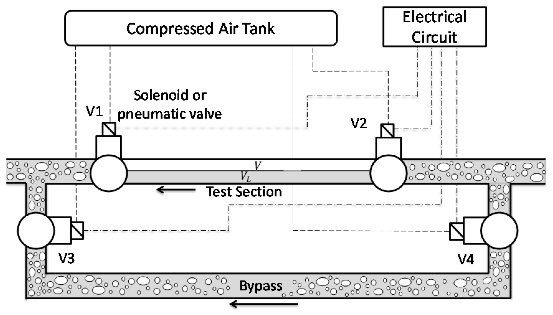
2.1. Quick-Closing Valves
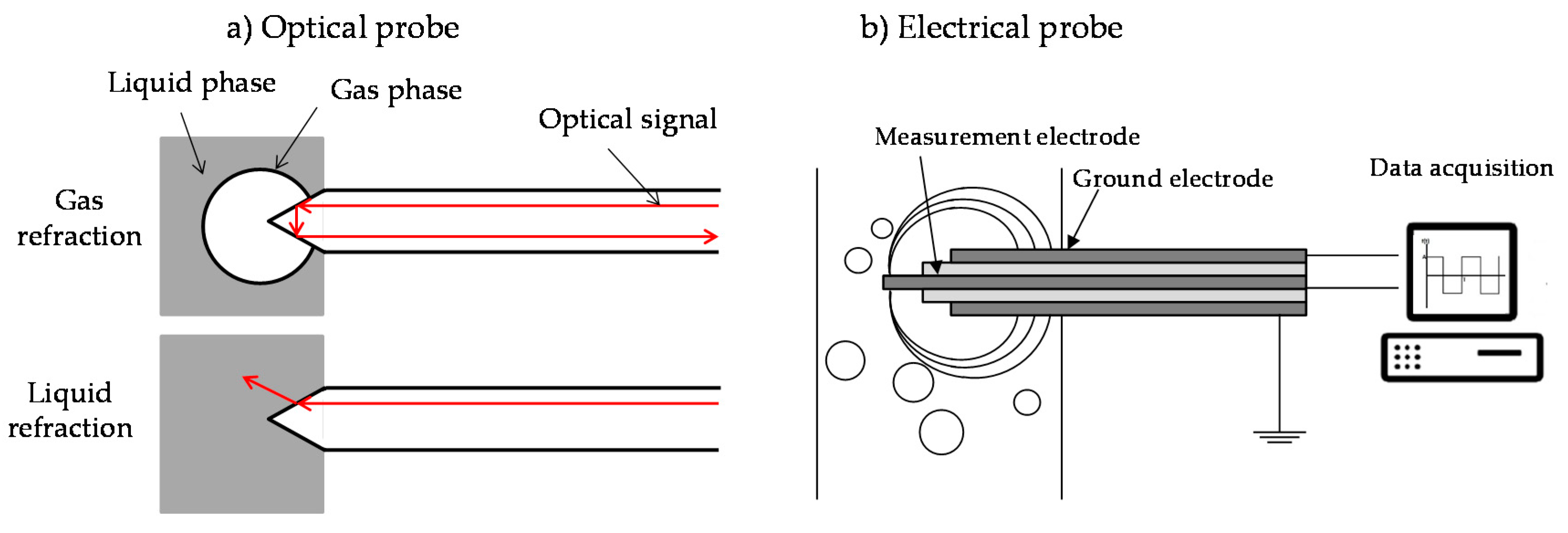
2.2. Local Measurements (Needle Probe)
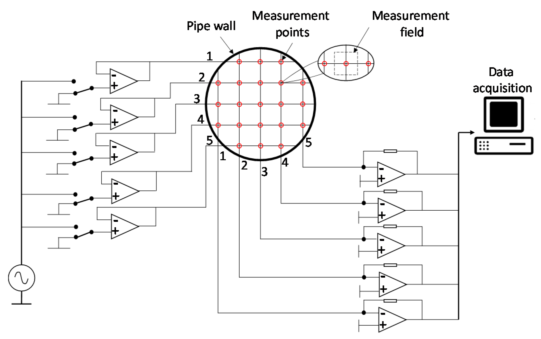
2.3. Wire-Mesh Sensor
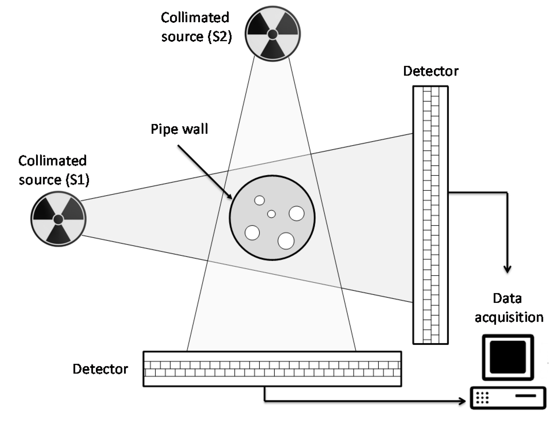
2.4. Hard-Field Tomography
2.5. Electrical Impedance Tomography
2.6. Photographic Image Technique
2.7. PIV
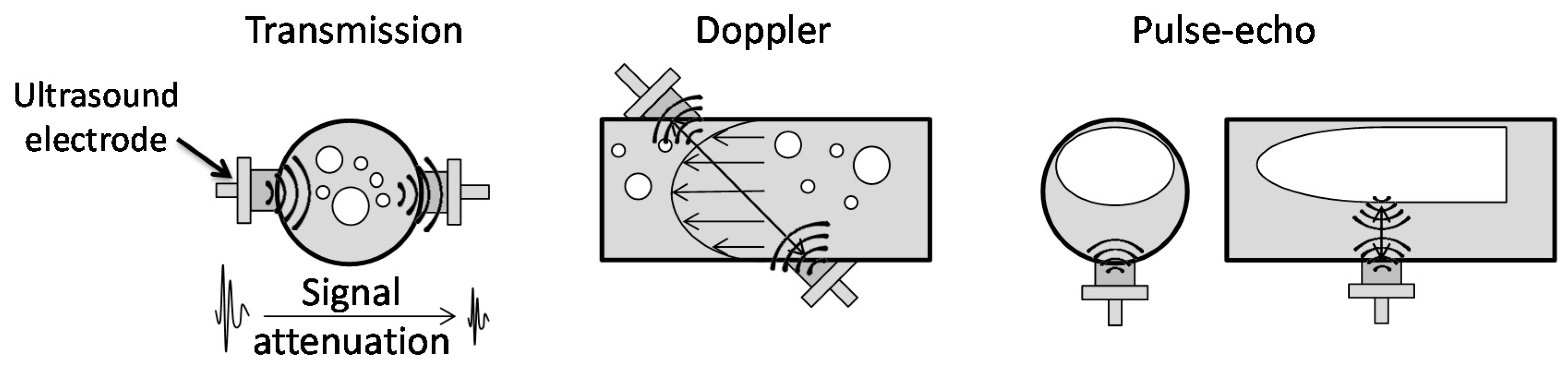
2.8. Ultrasound
2.9. Pressure Drop
2.10. Methods Comparison
- -
- keep low uncertainty
- -
- be capable of measure superficial or volumetric void fraction
- -
- not intrusive
- -
- able to measure instantaneous void fraction
3. Database
4. Void Fraction Correlations
4.1. Correlation Description
4.2. New Correlation
4.3. Results
5. Conclusions
- -
- In total, 18 measurement techniques for two-phase void fraction methods have been identified in the literature, classified in four main groups according to their measurement principle (mechanical, optical, electrical and ionizing radiation) and evaluated for their suitability for microchannel measurements.
- -
- Optical void fraction measurement techniques seem to aggregate most of the characteristics needed for high quality void fraction measurements in microchannels, allowing further reduction in channel diameter with lower cost and lower uncertainty compared to other techniques.
- -
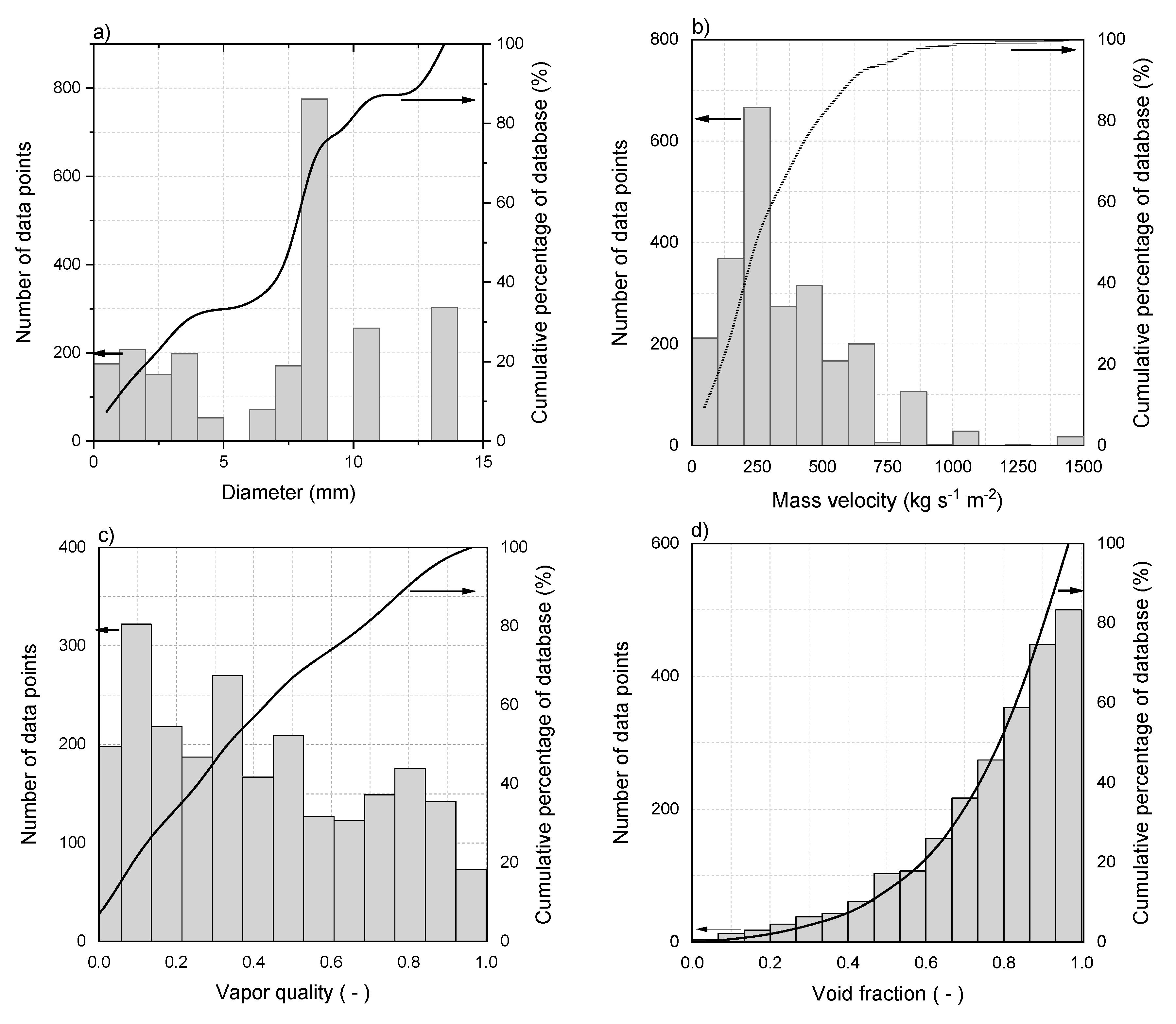
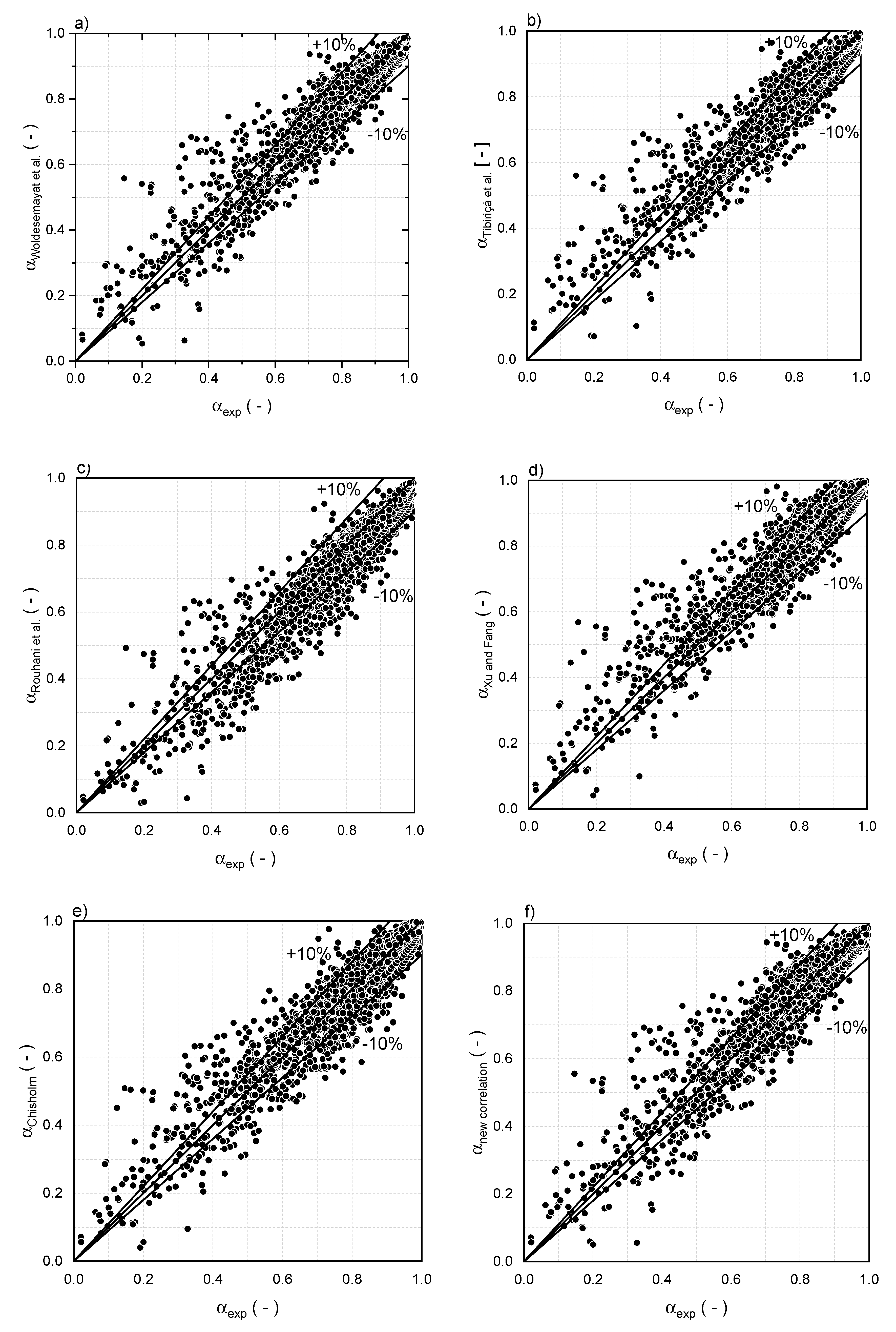
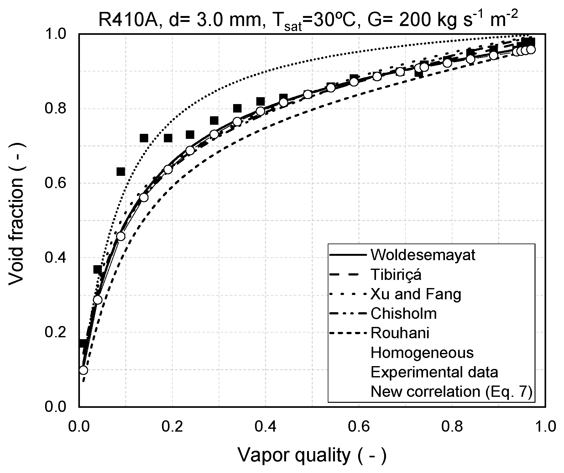
- A large void fraction database consisting of diabatic and adiabatic experimental data from the literature has been obtained for small-diameter channels (0.5 < D < 13.84 mm). This database was used for comparing well know void fraction correlations from literature against new proposed ones.
- -
- A new drift flux void fraction correlation was numerically adjusted with microchannel database containing 731 datapoints (0.5 < D < 3.0 mm) to test if predictions could be further improved. The new correlation could best predicted microchannel database and also the complete small channel diameter database of 2361 datapoints (0.5 < D < 13.84 mm) with mean absolute error of 7.9%. From the observed performance of the new correlation it can be concluded that the optimization of void fraction correlations for small scale diameters channels has not yet reached the limit and there is still space for improvement for new correlations, mainly in microchannels conditions.
Author Contributions
Funding
Acknowledgments
Conflicts of Interest
References
- Tibiriçá, C.B.; Ribatski, G. Flow boiling phenomenological differences between micro-and macroscale channels. Heat Transf. Eng. 2015, 36, 937–942. [Google Scholar] [CrossRef]
- Tibiriçá, C.B.; Rocha, D.M.; Sueth, I.L.S., Jr.; Bochio, G.; Shimizu, G.K.K.; Barbosa, M.C.; dos Santos Ferreira, S. A complete set of simple and optimized correlations for microchannel flow boiling and two-phase flow applications. Appl. Therm. Eng. 2017, 126, 774–795. [Google Scholar] [CrossRef]
- Tibirica, C.B.; Ribatski, G. Flow boiling in micro-scale channels–Synthesized literature review. Int. J. Refrig. 2013, 36, 301–324. [Google Scholar] [CrossRef]
- Chexal, B.; Horowitz, J.; Lellouche, G.S. An assessment of eight void fraction models. Nucl. Eng. Des. 1991, 126, 71–88. [Google Scholar] [CrossRef]
- Woldesemayat, M.A.; Ghajar, A.J. Comparison of void fraction correlations for different flow patterns in horizontal and upward inclined pipes. Int. J. Multiph. Flow 2007, 33, 347–370. [Google Scholar] [CrossRef]
- Cioncolini, A.; Thome, J.R. Void fraction prediction in annular two-phase flow. Int. J. Multiph. Flow 2012, 43, 72–84. [Google Scholar] [CrossRef]
- Lockhart, R.W.; Martinelli, R.C. Proposed correlation of data for isothermal two-phase, two-component flow in pipes. Chem. Eng. Prog 1949, 45, 39–48. [Google Scholar]
- Xu, Y.; Fang, X. Correlations of void fraction for two-phase refrigerant flow in pipes. Appl. Therm. Eng. 2014, 64, 242–251. [Google Scholar] [CrossRef]
- Jin, G.; Yan, C.; Sun, L.; Xing, D.; Zhou, B. Void fraction of dispersed bubbly flow in a narrow rectangular channel under rolling conditions. Prog. Nucl. Energy 2014, 70, 256–265. [Google Scholar] [CrossRef]
- Hashizume, K. Flow pattern, void fraction and pressure drop of refrigerant two-phase flow in a horizontal pipe—I. Experimental data. Int. J. Multiph. Flow 1983, 9, 399–410. [Google Scholar] [CrossRef]
- Schrage, D.S.; Hsu, J.T.; Jensen, M.K. Two-phase pressure drop in vertical crossflow across a horizontal tube bundle. Aiche J. 1988, 34, 107–115. [Google Scholar] [CrossRef]
- Xu, G.P.; Tso, C.P.; Tou, K.W. Hydrodynamics of two-phase flow in vertical up and down-flow across a horizontal tube bundle. Int. J. Multiph. Flow 1998, 24, 1317–1342. [Google Scholar] [CrossRef]
- Wilson, M.J.; Newell, T.A.; Chato, J.C. Experimental Investigation of Void Fraction during Horizontal Flow in Larger Diameter Refrigeration Applications; ACRC Technical Report 140; College of Engineering, University of Illinois at Urbana-Champaign: Urbana, IL, USA, 1998. [Google Scholar]
- Yashar, D.A.; Newell, T.A.; Chato, J.C. Experimental Investigation of Void Fraction during Horizontal Flow in Smaller Diameter Refrigeration Applications; ACRC Project 74; College of Engineering, University of Illinois at Urbana-Champaign: Urbana, IL, USA, 1998. [Google Scholar]
- Koyama, S.; Lee, J.; Yonemoto, R. An investigation on void fraction of vapor–liquid two-phase flow for smooth and microfin tubes with R134a at adiabatic condition. Int. J. Multiph. Flow 2004, 30, 291–310. [Google Scholar] [CrossRef]
- Srisomba, R.; Mahian, O.; Dalkilic, A.S.; Wongwises, S. Measurement of the void fraction of R-134a flowing through a horizontal tube. Int. Commun. Heat Mass Transf. 2014, 56, 8–14. [Google Scholar] [CrossRef]
- Zheng, Y.; Zhang, Q. Simultaneous measurement of gas and solid holdups in multiphase systems using ultrasonic technique. Chem. Eng. Sci. 2004, 59, 3505–3514. [Google Scholar] [CrossRef]
- Murakawa, H.; Kikura, H.; Aritomi, M. Application of ultrasonic Doppler method for bubbly flow measurement using two ultrasonic frequencies. Exp. Therm. Fluid Sci. 2005, 29, 843–850. [Google Scholar] [CrossRef]
- Vasconcelos, A.M.; Carvalho, R.D.M.; Venturini, O.J.; França, F.A. The use of the ultrasonic technique for void fraction measurements in air-water bubbly flows. In Proceedings of the 11th Brazilian Congress of Thermal Sciences and Engineering, Curitiba, Brazil, 5–8 December 2006. [Google Scholar]
- Jia, J.; Babatunde, A.; Wang, M. Void fraction measurement of gas–liquid two-phase flow from differential pressure. Flow Meas. Instrum. 2015, 41, 75–80. [Google Scholar] [CrossRef]
- Revellin, R.; Dupont, V.; Ursenbacher, T.; Thome, J.R.; Zun, I. Characterization of diabatic two-phase flows in microchannels: Flow parameter results for r-134a in a 0.5 mm channel. Int. J. Multiph. Flow 2006, 32, 755–774. [Google Scholar] [CrossRef]
- Sempértegui-Tapia, D.; De Oliveira Alves, J.; Ribatski, G. Two-phase flow characteristics during convective boiling of halocarbon refrigerants inside horizontal small-diameter tubes. Heat Transf. Eng. 2013, 34, 1073–1087. [Google Scholar] [CrossRef]
- Harada, K.; Murakami, M.; Ishii, T. PIV measurements for flow pattern and void fraction in cavitating flows of He II and He I. Cryogenics 2006, 46, 648–657. [Google Scholar] [CrossRef]
- Dowlati, R.; Kawaji, M.; Chisholm, D.; Chan, A.M. Void fraction prediction in two-phase flow across a tube bundle. AI Ch. E. J. 1992, 38, 619–622. [Google Scholar] [CrossRef]
- Kendoush, A.A.; Sarkis, Z.A. Void fraction measurement by X-ray absorption. Exp. Therm. Fluid Sci. 2002, 25, 615–621. [Google Scholar] [CrossRef]
- Mishima, K.; Hibiki, T. Some characteristics of air-water two-phase flow in small diameter vertical tubes. Int. J. Multiph. Flow 1996, 22, 703–712. [Google Scholar] [CrossRef]
- Portillo, G.; Shedd, T.A.; Lehrer, K.H. Void fraction measurement in minichannels with in- situ calibration. In Proceedings of the International Refrigeration and Air Conditioning Conference; University of Wisconsin-Madison, Department of Mechanical Engineering: Madison, WI, USA, 2008. [Google Scholar]
- Paranjape, S.; Ritchey, S.N.; Garimella, S.V. Electrical impedance-based void fraction measurement and flow regime identification in microchannel flows under adiabatic conditions. Int. J. Multiph. Flow 2012, 42, 175–183. [Google Scholar] [CrossRef]
- Shedd, T.A. Void Fraction and Pressure Drop Measurements for Refrigerant r410a Flows in Small Diameter Tubes; Technical Report 20110-01; University of Wisconsin: Madison, WI, USA, 2012. [Google Scholar]
- Olivier, S.P.; Meyer, J.P.; De Paepe, M.; De Kerpel, K. The influence of inclination angle on void fraction and heat transfer during condensation inside a smooth tube. Int. J. Multiph. Flow 2016, 80, 1–14. [Google Scholar] [CrossRef]
- De Kerpel, K.; Ameel, B.; De Schampheleire, S.; T’Joen, C.; Canière, H.; De Paepe, M. Calibration of a capacitive void fraction sensor for small diameter tubes based on capacitive signal features. Appl. Therm. Eng. 2014, 63, 77–83. [Google Scholar] [CrossRef]
- Barreto, E.X.; Oliveira, J.L.G.; Passos, J.C. Frictional pressure drop and void fraction analysis in air–water two-phase flow in a microchannel. Int. J. Multiph. Flow 2015, 72, 1–10. [Google Scholar] [CrossRef]
- Zhou, Y.; Chang, H.; Lv, Y. Gas-liquid two-phase flow in a horizontal channel under nonlinear oscillation: Flow regime, frictional pressure drop and void fraction. Exp. Therm. Fluid Sci. 2019, 109, 109852. [Google Scholar] [CrossRef]
- Huang, S.; Zhang, X.; Wang, D.; Lin, Z. Equivalent water layer height (EWLH) measurement by a single-wire capacitance probe in gas–liquid flows. Int. J. Multiph. Flow 2008, 34, 809–818. [Google Scholar] [CrossRef]
- He, D.; Chen, S.; Bai, B. Void fraction measurement of stratified gas-liquid flow based on multi-wire capacitance probe. Exp. Therm. Fluid Sci. 2019, 102, 61–73. [Google Scholar] [CrossRef]
- Netto, J.F.; Fabre, J.; Peresson, L. Shape of long bubbles in horizontal slug flow. Int. J. Multiph. Flow 1999, 25, 1129–1160. [Google Scholar] [CrossRef]
- Oddie, G.; Shi, H.; Durlofsky, L.J.; Aziz, K.; Pfeffer, B.; Holmes, J.A. Experimental study of two and three phase flows in large diameter inclined pipes. Int. J. Multiph. Flow 2003, 29, 527–558. [Google Scholar] [CrossRef]
- Morris, D.; Teyssedou, A.; Lapierre, J.; Tapucu, A. Optical fiber probe to measure local void fraction profiles. Appl. Opt. 1987, 26, 4660–4664. [Google Scholar] [CrossRef] [PubMed]
- Graindorge, P.; Le Boudec, G.; Meyet, D.; Arditty, H.J. High bandwidth two-phase flow void fraction fiber optic sensor. In Fiber Optic Sensors I. Int. Soc. Opt. Photonics 1986, 586, 211–215. [Google Scholar]
- Spindler, K.; Bierer, M.; Lorenz, G.; Erhard, A.; Hahne, E. Measurements in vertical gas-liquid two-phase flows using an optical fiber probe. In Proceedings of the 1st World Conference on Experimental Heat Transfer, Fluid Mechanics and Thermodynamics, Dubrovnik, Croatia, 4–9 September 1988; pp. 348–357. [Google Scholar]
- Danel, F. Local measurement in two-phase flow: Recent optical probe design developments. Houille Blanche 1978, 351–355. [Google Scholar] [CrossRef]
- Murzyn, F.; Mouazé, D.; Chaplin, J.R. Optical fiber probe measurements of bubbly flow in hydraulic jumps. Int. J. Multiph. Flow 2005, 31, 141–154. [Google Scholar] [CrossRef]
- Da Silva, M.J.; Schleicher, E.; Hampel, U. A novel needle probe based on high-speed complex permittivity measurements for investigation of dynamic fluid flows. IEEE Trans. Instrum. Meas. 2007, 56, 1249–1256. [Google Scholar] [CrossRef]
- Cartellier, A.; Achard, J.L. Local phase detection probes in fluid/fluid two-phase flows. Rev. Sci. Instrum. 1991, 62, 279–303. [Google Scholar] [CrossRef]
- Da Silva, M.J. Instrumentação em Escoamentos Multifásicos. In Proceedings of the 4th EBEM, São Paulo, Brazil; 27–31 March 2017; Escola Brasileira de Escoamento Multifásico: São Paulo, Brazil, 2017. [Google Scholar]
- Prasser, H.M.; Böttger, A.; Zschau, J. A new electrode-mesh tomograph for gas–liquid flows. Flow Meas. Instrum. 1998, 9, 111–119. [Google Scholar] [CrossRef]
- Da Silva, M.J.; Schleicher, E.; Hampel, U. Capacitance wire-mesh sensor for fast measurement of phase fraction distributions. Meas. Sci. Technol. 2007, 18, 2245–2251. [Google Scholar] [CrossRef]
- Pietruske, H.; Prasser, H.M. Wire-mesh sensors for high-resolving two-phase flow studies at high pressures and temperatures. Flow Meas. Instrum. 2007, 18, 87–94. [Google Scholar] [CrossRef]
- Manera, A.; Prasser, H.M.; Lucas, D.; Van Der Hagen, T.H.J.J. Three-dimensional flow pattern visualization and bubble size distributions in stationary and transient upward flashing flow. Int. J. Multiph. Flow 2006, 32, 996–1016. [Google Scholar] [CrossRef]
- Peña, H.V.; Rodriguez, O.M.H. Applications of wire-mesh sensors in multiphase flows. Flow Meas. Instrum. 2015, 45, 255–273. [Google Scholar] [CrossRef]
- Yang, W.Q.; Spink, D.M.; York, T.A.; McCann, H.J.M.S. An image-reconstruction algorithm based on Landweber’s iteration method for electrical-capacitance tomography. Meas. Sci. Technol. 1999, 10, 1065. [Google Scholar] [CrossRef]
- Yang, W.Q.; Peng, L. Image reconstruction algorithms for electrical capacitance tomography. Meas. Sci. Technol. 2002, 14, R1–R13. [Google Scholar] [CrossRef]
- Widyatama, A.; Dinaryanto, O. The development of image processing technique to study the interfacial behavior of air-water slug two-phase flow in horizontal pipes. Flow Meas. Instrum. 2018, 59, 168–180. [Google Scholar] [CrossRef]
- Wojtan, L.; Ursenbacher, T.; Thome, J.R. Interfacial measurements in stratified types of flow. Part II: Measurements for R-22 and R-410A. Int. J. Multiph. Flow 2004, 30, 125–137. [Google Scholar] [CrossRef]
- Povolny, A.; Kikura, H.; Ihara, T. Ultrasound pulse-echo coupled with a tracking technique for simultaneous measurement of multiple bubbles. Sensors 2018, 18, 1327. [Google Scholar] [CrossRef]
- Aritomi, M.; Zhou, S.; Takeda, Y.; Nakamura, H.; Kukita, Y. Measurement of Bubbly Flows in Vertical Channels Using Ultrasonic Velocity Profile Monitor; International Atomic Energy Agency (IAEA): Vienna, Austria, 1998. [Google Scholar]
- Wallis, G.B. Use of the Reynolds Flux Concept for Analysing One-Dimensional Two-Phase Flow. Int. J. Heat Mass Transf. 1969, 11, 445–458. [Google Scholar] [CrossRef]
- Tang, C.; Heindel, T.J. Similitude analysis for gas-liquid-fiber flows in co-current bubble columns. In Proceedings of the Fluids Engineering Division Summer Meeting, Miami, FL, USA, 17–20 July 2006; Volume 47500, pp. 1787–1798. [Google Scholar]
- Keinath, B.L. Void Fraction, Pressure Drop, and Heat Transfer in High Pressure Condensing Flows through Microchannels. Ph.D. Thesis, Georgia Institute of Technology, Atlanta, GA, USA, 2012. [Google Scholar]
- Kandlikar, S.G. Fundamental issues related to flow boiling in minichannels and microchannels. Exp. Therm. Fluid Sci. 2002, 26, 389–407. [Google Scholar] [CrossRef]
- Lips, S.; Meyer, J.P. Experimental study of convective condensation in an inclined smooth tube. Part I: Inclination effect on flow pattern and heat transfer coefficient. Int. J. Heat Mass Transf. 2012, 55, 395–404. [Google Scholar] [CrossRef]
- Milkie, J.A.; Garimella, S.; Macdonald, M.P. Flow regimes and void fractions during condensation of hydrocarbons in horizontal smooth tubes. Int. J. Heat Mass Transf. 2016, 92, 252–267. [Google Scholar] [CrossRef]
- Wojtan, L. Experimental and Analytical Investigation of Void Fraction and Heat Transfer during Evaporation in Horizontal Tubes. Ph.D. Thesis, Ecole Polytechnique Federale de Lausanne (EPFL), Lausanne, Switzerland, 2004. [Google Scholar]
- Canière, H. Flow Pattern Mapping of Horizontal Evaporating Refrigerant Flow Based on Capacitive Void Fraction Measurements. Ph.D. Thesis, Ghent University, Ghent, Belgium, 2009. [Google Scholar]
- Graham, D.M. Experimental Investigation of Void Fraction during Refrigerant Condensation; Technical Report ACRC Project 74; College of Engineering, University of Illinois at Urbana-Champaign: Urbana, IL, USA, 1997. [Google Scholar]
- Kopke, H.R. Experimental Investigation of Void Fraction during Refrigerant Condensation in Horizontal Tubes; Air Conditioning and Refrigeration Center, College of Engineering, University of Illinois at Urbana-Champaign: Urbana, IL, USA, 1998. [Google Scholar]
- Hughmark, G.A. Holdup and heat transfer in horizontal slug gas-liquid flow. Chem. Eng. Sci. 1965, 20, 1007–1010. [Google Scholar] [CrossRef]
- Rouhani, S.Z.; Axelsson, E. Calculation of void volume fraction in the subcooled and quality boiling regions. Int. J. Heat Mass Transf. 1970, 13, 383–393. [Google Scholar] [CrossRef]
- Zuber, N.; Findlay, J. Average volumetric concentration in two-phase flow systems. J. Heat Transf. 1965, 87, 453–468. [Google Scholar] [CrossRef]
- Dix, G.E. Vapor Void Fractions for Forced Convection with Subcooled Boiling at Low Flow Rates. Ph.D. Thesis, University of California, Berkeley, CA, USA, 1971. [Google Scholar]
- Chisholm, D. Pressure gradients due to friction during the flow of evaporating two-phase mixtures in smooth tubes and channels. Int. J. Heat Mass Transf. 1973, 16, 347–358. [Google Scholar] [CrossRef]
- Domanski, P.A.; Didion, D. Computer Modeling of the Vapor Compression Cycle with Constant Flow Area Expansion Device; National Institute of Standards and Technology (NIST): Washington, DC, USA, 1983. [Google Scholar]
- Spedding, P.L.; Chen, J.J.J. Holdup in two phase flow. Int. J. Multiph. Flow 1984, 10, 307–339. [Google Scholar] [CrossRef]
- Kariyasaki, A.; Fukano, T.; Kagawa, M. Characteristics of Time Varying Void Fraction in Isothermal Air-Water Concurrent Flow in a Horizontal Capillary Tube. In Proceedings of the 1991 ASME JSME Thermal Engineering Joint Conference, Reno, NV, USA, 17–22 March 1991. [Google Scholar]
- Graham, D.M.; Kopke, H.R.; Wilson, M.J.; Yashar, D.A.; Chato, J.C.; Newell, T.A. An Investigation of Void Fraction in the Stratified/Annular Flow Regions in Smooth, Horizontal Tubes; Air Conditioning and Refrigeration Center, College of Engineering, University of Illinois at Urbana-Champaign: Urbana, IL, USA, 1999. [Google Scholar]
- Niño, V.G.; Hrnjak, P.S.; Newell, T.A. Characterization of Two-Phase Flow in Microchannels; Air Conditioning and Refrigeration Center, College of Engineering, University of Illinois at Urbana-Champaign: Urbana, IL, USA, 2002. [Google Scholar]
- Kawahara, A.; Sadatomi, M.; Okayama, K.; Kawaji, M.; Chung, P.Y. Effects of channel diameter and liquid properties on void fraction in adiabatic two-phase flow through microchannels. Heat Transf. Eng. 2005, 26, 13–19. [Google Scholar] [CrossRef]
- Zhang, W.; Hibiki, T.; Mishima, K. Correlations of two-phase frictional pressure drop and void fraction in mini-channel. Int. J. Heat Mass Transf. 2010, 53, 453–465. [Google Scholar] [CrossRef]
- Kanizawa, F.T.; Ribatski, G. Void fraction predictive method based on the minimum kinetic energy. J. Braz. Soc. Mech. Sci. Eng. 2016, 38, 209–225. [Google Scholar] [CrossRef]
- Karayiannis, T.G.; Mahmoud, M.M. Flow boiling in microchannels: Fundamentals and applications. Appl. Therm. Eng. 2017, 115, 1372–1397. [Google Scholar] [CrossRef]


| Principle | Technique | Authors | D [mm] | Fluid | Type |
|---|---|---|---|---|---|
| Mechanical | Quick-closing valves | Hashizume [10] | 10.0 | R12; R22 | Evap. |
| Schrage et al. [11] | 7.94 | Water-air | Adiab. | ||
| Xu et al. [12] | 9.79 | Water-air | Adiab. | ||
| Wilson [13] | 6.12 | R134a; R410A | Evap. | ||
| Yashar et al. [14] | 4.26 | R410A | Evap. | ||
| Koyama et al. [15] | 7.52 | R134a | Adiab. | ||
| Srisomba et al. [16] | 8.0 | R134a | Adiab. | ||
| Ultrasound | Zheng and Zhang [17] | 76.0 | Water | Adiab. | |
| Murakawa et al. [18] | 50.0 | Water (with nylon)-air | Adiab. | ||
| Vasconcelos et al. [19] | 54.0 | Water-air | Adiab. | ||
| Pressure drop | Jia et al. [20] | 50.0 | Water-air | Adiab. | |
| Optical | Light | Revellin et al. [21] | 0.5 | R134a | Evap. |
| Laser | Sempértegui-Tapia et al. [22] | 1.1; 2.32 | R134a; R245fa | Adiab. | |
| Particle Image Velocimetry (PIV) | Harada and Murakami [23] | n/d | He II; He I | n/d | |
| Ionizing radiation | Gamma-ray radiation | Dowlati et al. [24] | 12.7 | Water-air | Adiab. |
| X-ray radiation | Kendoush and Sarkis [25] | 28.0; 36.0 | Water-air | Adiab. Diab. | |
| Neutron emission | Mishima and Hibiki [26] | 1.05 | Water-air | n/d | |
| Electrical | Capacitive (ring sensor) | Portillo et al. [27] | 3.0 | R410A | Evap. |
| Impedance | Paranjape et al. [28] | 0.78 | Water-air | Adiab. | |
| Capacitive (Annular sensor) | Shedd [29] | 0.508 | R410A | Cond. | |
| Olivier et al. [30] | 8.38 | R134a | Cond. | ||
| Capacitive (concave sensor) | De Kerpel et al. [31] | 8.0 | R134a, R410A | Adiab. | |
| Resistive | Barreto et al. [32] | 1.2 | Water-air | Adiab. | |
| Capacitively coupled contactless conductivity detection () | Zhou [33] | 2.8; 3.9 | Water-nitrogen | Adiab. | |
| Single-wire capacitance probe | Huang et al. [34] | 29 | Water-air | Adiab. | |
| Multi-wire capacitance probe | He et al. [35] | 50 | Water-air | Adiab. | |
| Netto and Peresson [36] | 53 | Water-air | Adiab. |
| Technique | Spatial Resolution | Temporal Resolution | Costs | Observation |
|---|---|---|---|---|
| Quick-closing valve | Good | No | Low | Intrusive, microchannel |
| Needle probes (electrical, optical) | No | Good | Low | Intrusive, local measurement |
| Ultrasound probe | No | High | Medium | Measures average void fraction |
| Optical (PIV, LDA, videometry) | High | High | Medium | Low gas fraction |
| Hard-field tomography (X-ray, , PET, MRI) | Good | Low | High | Radiation protection |
| Soft-field (EIT, ECT, ERT) | Low | High | Low | Nonlinear |
| Wire-mesh sensor | High | High | Low | Intrusive |
| Authors | Technique | D [mm]/Geometry | Fluid | Type/Orientation | Data Points | Uncertainty |
|---|---|---|---|---|---|---|
| Shedd [29] | Capacitive sensor | 0.508, 1.19, 2.92/C | R410A | Cond./H | 444 | 5% |
| Revellin et al. [21] | Light | 0.5/C | R134a | Evap./H | 10 | n/d |
| Portillo et al. [27] | Capacitive sensor | 3.0/C | R410A | Evap./H | 64 | n/d |
| Keinath [59] | Image | 0.51, 1.0.3.0/C | R404A | Cond./H | 176 | 2–30.6% |
| Barreto et al. [32] | Resistive sensor | 1.2/C | Air-water | Adiab./V | 37 | 5% |
| Authors | Technique | D [mm]/Geometry | Fluid | Type/Orientation | Data Points | Uncertainty |
|---|---|---|---|---|---|---|
| Yashar et al. [14] | Quick-closing valves | 4.26, 7.25, 7.26/C | R134a, R410A | Evap. Adiab./H | 57 | 0.3% |
| Srisomba et al. [16] | Quick-closing valves | 8.0/C | R134a | Adiab./H | 117 | 1.2% |
| Lips and Meyer [61] | Pressure drop | 8.38/C | R134a | Cond./−90° to 90° | 6 | n/d |
| Milkie et al. [62] | Image | 7.0/C | Propane | Cond./H | 83 | n/d |
| Olivier et al. [30] | Capacitive sensor | 8.38/C | R134a | Cond./−90° to 90° | 23 | 2% |
| Hashizume [10] | Quick-closing valves | 10.0/C | R12, R22 | Evap./H | 256 | n/d |
| Wilson [13] | Quick-closing valves | 6.12, 8.89/C | Propane | Cond./H | 94 | 0.3–5.0% |
| Wojtan [63] | Image | 8.0, 13.84/C | R22, R410A | Evap./H | 328 | 1.0–3.0% |
| De Kerpel et al. [31]. | Capacitive sensor | 8.0/C | R134a, R410A | Adiab./H | 270 | 1.3% |
| Canière [64] | Capacitive sensor | 8.0/C | R134a, R410A | Evap./H | 279 | 10% |
| Graham [65] | Quick-closing valves | 7.04/C | R134a, R410A | Cond./H | 40 | n/d |
| Kopke [66] | Quick-closing valves | 6.04, 7.04/C | R134a, R410A | Cond. Adiab. Evap./H | 44 | 10% |
| Koyama et al. [15] | Quick-closing valves | 7.52/C | R134a | Adiab./H | 28 | 0.7–6.2% |
| Diameter/Condition | R134a | R404A | R410A | Propane | R12 | R22 | Air-Water | |
|---|---|---|---|---|---|---|---|---|
| d < 3.0 mm | Data points | 10 | 176 | 508 | n/d | n/d | n/d | 37 |
| % | 1.37 | 69.49 | 24.08 | n/d | n/d | n/d | 5.06 | |
| d > 3.0 mm | Data points | 477 | n/d | 549 | 117 | 104 | 323 | n/d |
| % | 29.26 | n/d | 33.68 | 10.86 | 6.38 | 19.82 | n/d | |
| All database | Data points | 487 | 176 | 1057 | 177 | 104 | 323 | 37 |
| % | 20.62 | 7.45 | 44.77 | 7.50 | 4.41 | 13.68 | 1.57 | |
| Model Type | Authors | Correlation | Comments |
|---|---|---|---|
| Homogeneous | Homogeneous | ||
| Slip ratio | Lockhart and Martinelli [7] | Based on air-water flowing in 1.5 < d < 25.8 mm horizontal tube. | |
| Chisholm [71] | Derived a slip model for annular flow based on the homogeneous model with approximately equal frictional pressure drop in both phases | ||
| Spedding and Chen [73] | Based on air-water upward and downward inclined flow orientation. | ||
| Xu and Fang [8] | Based on 1574 data points. 0.5 < d < 10 mm; 40 < G < 1000 kg s−1 m−2; R11, R12, R134a and R410A | ||
| Tibiriçá et al. [2] | Based on 1433 data points for horizontal flow. 0.508 < d < 13.84 mm; 40 < G < 1000 kg s−1 m−2; R22, R134a, R404A and R410A. | ||
| Drif flux | Hughmark [67] | ||
| Rouhani and Axelsson [68] | Correlation adjusted based on Zuber and Findlay [67] drift flux model | ||
| Dix [70] | |||
| Woldesemayat and Ghajar [5] | Based on 2845 data points for horizontal, vertical, and inclined flow for 12.7 < d < 102.26 mm flowing natural gas-water, air-water and air-kerosene | ||
| Zhang [78] | Based in air-water flowing in 0.2 < d < 4.9 mm at atmospheric pressure. | ||
| Kawahara et al. [77] | , For | Based on homogeneous void fraction model. The coefficients were adjusted for horizontal flow, 0.05 < d < 0.25 mm, water-nitrogen and ethanol/water-nitrogen | |
| Miscellaneous | Wallis [57] | , | Based on Lockhart and Matinelli [7] multipliers. 1.5 < d < 25.8 mm |
| Domanski and Didion [72] | Based on Wallis [57] correlation | ||
| Kariyasaki et al. [74] | Based on tests with air-water in isothermal ducts with 1.0 < d < 4.9 mm; and are constants dependents of the tube diameter. | ||
| Graham [75] | , | Based on 40 data points for horizontal flow. d = 7.04 mm; 75 < G < 450 kg s−1 m−2; R134a and R410A | |
| Nino [76] | , | Based on 6 and 14 port-microchannel with hydraulic diameter of 1.58 and 1.02 mm, respectively, for horizontal flow. 50 < G < 300 kg s−1 m−2; air-water, R134a and R410A. | |
| Shedd [29] | Based on 444 data points for horizontal flow. 0.508 < d < 2.92 mm; 200 < G < 800 kg s−1 m−2; R410A | ||
| Cioncolini and Thome [6] | , | Based on 2673 data points, where 94.3% of the data are for horizontal flow. 1.05 < d < 45.5 mm; 22 < G < 3420 kg s−1 m−2; water-steam, R410A, water-air, water-argon, water-nitrogen, water-alcohol-air, alcohol-air and kerosene-air | |
| Kanizawa et al. [79] | Based on the principle of minimum kinetic energy. The coefficients were adjusted based on database for horizontal and vertical upward flows. 0.5 < d < 89 mm; 37 < G < 4500 kg s−1 m−2; R12, R22, R134a, R410A, air-water, air-kerosene and air-glycerin |
| Ahors | (%) | λ10% (%) |
|---|---|---|
| Homogeneous | 15.91 | 51.35 |
| Lockhart and Martinelli [7] | 14.89 | 66.65 |
| Hughmark [67] | 12.51 | 45.05 |
| Wallis [57] | 16.03 | 68.64 |
| Rouhani and Axelsson [68] | 8.88 | 76.08 |
| Dix [70] | 11.44 | 63.02 |
| Chisholm [71] | 8.28 | 78.57 |
| Domanski and Didion [72] | 15.36 | 68.81 |
| Spedding and Chen [73] | 15.31 | 39.77 |
| Kariyasaki et al. [74] | 15.70 | 29.75 |
| Graham [75] | 11.08 | 76.54 |
| Nino [76] | 29.44 | 55.49 |
| Kawahara et al. [77] | 44.45 | 11.83 |
| Woldesemayat and Ghajar [5] | 7.98 | 81.11. |
| Zhang [78] | 13.05 | 43.66 |
| Shedd [29] | 13.57 | 62.76 |
| Cioncolini and Thome [6] | 13.37 | 66.57 |
| Xu and Fang [8] | 8.22 | 80.60 |
| Kanizawa et al. [79] | 9.23 | 82.54 |
| Tibiriçá et al. [2] | 8.16 | 82.67 |
| New correlation (Equation (7)) | 7.90 | 79.46 |
| Authors | (%) | λ10% (%) |
|---|---|---|
| Homogeneous | 16.47 | 46.75 |
| Lockhart and Martinelli [7] | 11.70 | 67.48 |
| Hughmark [67] | 11.70 | 49.69 |
| Wallis [57] | 11.83 | 70.60 |
| Rouhani and Axelsson [68] | 8.15 | 80.31 |
| Dix [70] | 10.99 | 65.28 |
| Chisholm [71] | 7.16 | 84.05 |
| Domanski and Didion [72] | 11.66 | 70.18 |
| Spedding and Chen [73] | 12.82 | 48.04 |
| Kariyasaki et al. [74] | 14.93 | 33.19 |
| Graham [75] | 7.14 | 81.96 |
| Nino [76] | 20.61 | 61.59 |
| Kawahara et al. [77] | 40.06 | 14.91 |
| Woldesemayat and Ghajar [5] | 6.78 | 84.29 |
| Zng [78] | 11.70 | 49.69. |
| Shedd [29] | 13.75 | 60.98 |
| Cioncolini and Thome [6] | 11.65 | 66.07 |
| Xu and Fang [8] | 7.22 | 83.62 |
| Kanizawa et al. [79] | 6.99 | 86.56 |
| Tibiriçá et al. [2] | 6.47 | 85.83 |
| New correlation (Equation (7)) | 7.04 | 81.78 |
| Authors | (%) | λ10% (%) |
|---|---|---|
| Homogeneous | 14.66 | 61.55 |
| Lockhart and Martinelli [7] | 21.95 | 64.84 |
| Hughmark [67] | 14.29 | 34.78 |
| Wallis [57] | 25.35 | 65.49 |
| Rouhani and Axelsson [68] | 10.50 | 66.71 |
| Dix [70] | 12.41 | 58.02 |
| Chisholm [71] | 10.76 | 66.44 |
| Domanski and Didion [72] | 23.53 | 65.76 |
| Spedding and Chen [73] | 20.82 | 65.76 |
| Kariyasaki et al. [74] | 17.42 | 22.15 |
| Graham [75] | 19.80 | 64.54 |
| Nino [76] | 48.99 | 41.98 |
| Kawahara et al. [77] | 54.16 | 5.03 |
| Woldesemayat and Ghajar [5] | 10.63 | 74.05 |
| Zhang [78] | 16.04 | 30.30 |
| Shedd [29] | 13.16 | 66.71 |
| Cioncolini and Thome [6] | 17.18 | 67.66 |
| Xu and Fang [8] | 10.43 | 73.91 |
| Kanizawa et al. [79] | 14.17 | 73.64 |
| Tibiriçá et al. [2] | 11.92 | 75.68 |
| New correlation (Equation (7)) | 9.80 | 74.32 |
| Authors | (%) |
|---|---|
| Shedd [29] | 6.98 |
| Revellin et al. [21] | 4.75 |
| Portillo et al. [27] | 9.55 |
| Keinath [59] | 16.17 |
| Barreto et al. [32] | 14.95 |
| Authors | (%) |
|---|---|
| Yashar et al. [14] | 2.41 |
| Srisomba et al. [16] | 18.37 |
| Lips and Meyer [61] | 3.64 |
| Milkie et al. [62] | 6.87 |
| Olivier et al. [30] | 1.94 |
| Hashizume [10] | 5.16 |
| Wilson [13] | 3.75 |
| Wojtan [63] | 7.96 |
| De Kerpel et al. [31]. | 2.70 |
| Canière [64] | 6.06 |
| Graham [65] | 6.42 |
| Kopke [66] | 10.06 |
| Koyama et al. [15] | 6.05 |
Publisher’s Note: MDPI stays neutral with regard to jurisdictional claims in published maps and institutional affiliations. |
© 2020 by the authors. Licensee MDPI, Basel, Switzerland. This article is an open access article distributed under the terms and conditions of the Creative Commons Attribution (CC BY) license (http://creativecommons.org/licenses/by/4.0/).
Share and Cite
Gardenghi, Á.R.; Filho, E.d.S.; Chagas, D.G.; Scagnolatto, G.; Oliveira, R.M.; Tibiriçá, C.B. Overview of Void Fraction Measurement Techniques, Databases and Correlations for Two-Phase Flow in Small Diameter Channels. Fluids 2020, 5, 216. https://doi.org/10.3390/fluids5040216
Gardenghi ÁR, Filho EdS, Chagas DG, Scagnolatto G, Oliveira RM, Tibiriçá CB. Overview of Void Fraction Measurement Techniques, Databases and Correlations for Two-Phase Flow in Small Diameter Channels. Fluids. 2020; 5(4):216. https://doi.org/10.3390/fluids5040216
Chicago/Turabian StyleGardenghi, Álvaro Roberto, Erivelto dos Santos Filho, Daniel Gregório Chagas, Guilherme Scagnolatto, Rodrigo Monteiro Oliveira, and Cristiano Bigonha Tibiriçá. 2020. "Overview of Void Fraction Measurement Techniques, Databases and Correlations for Two-Phase Flow in Small Diameter Channels" Fluids 5, no. 4: 216. https://doi.org/10.3390/fluids5040216
APA StyleGardenghi, Á. R., Filho, E. d. S., Chagas, D. G., Scagnolatto, G., Oliveira, R. M., & Tibiriçá, C. B. (2020). Overview of Void Fraction Measurement Techniques, Databases and Correlations for Two-Phase Flow in Small Diameter Channels. Fluids, 5(4), 216. https://doi.org/10.3390/fluids5040216