Assessment and Prediction of Air Entrainment and Geyser Formation in a Bottom Outlet: Field Observations and CFD Simulation

Abstract

Air entrainment at the intake of a bottom outlet often gives rise to air pockets in its conduit and formation of geysers. The outlet in question comprises a bulkhead gate, gate shaft, horizontal conduit, and exit. Operations show that it suffers from appreciable flow fluctuations and blowouts in the tailwater, which leads to gate operation restrictions. For the purpose of understanding the hydraulic phenomenon, both prototype discharge tests and three-dimensional computational fluid dynamics (CFD) modeling of two-phase flows are performed. The operational focus of the facility are small and large gate openings. The CFD results reveal that, with air entrained in the gate shaft, continual breakup and coalescence of air bubbles in the conduit typify the flow. At small openings below 1 meter, the air–water flow is characterized by either distinct blowouts of regular frequency or continuous air release. In terms of geyser behaviors inclusive of frequency, the agreement is good between field and numerical studies. At large openings, the gate becomes fully submerged, and the flow is discharged without air entrainment and blowouts. The paper showcases the air–water flow features in a typical bottom outlet layout in Sweden, which is intended to serve as an illustration of the study procedure for other similar outlets.

1. Introduction

A plunging jet often occurs in civil facilities like hydropower, irrigation, water treatment, and urban sewerage. When the water plunges with high velocity into a receiving pool, air gets entrained into the water, which is ascribable to the churn-turbulent mixing associated with water-surface irregularities, overturning and overlapping of water bodies at the impact location [1,2,3,4]. Often, the pool is confined by lateral boundaries, which augments the water-surface fluctuations and enhances the turbulent mixing [5,6,7]. Using a shadowgraph technique, Di Nunno et al. [8] address the deformation of air bubbles near a plunging jet. Some machine learning algorithms are developed for the prediction of air bubble shape and size. The study provides a promising approach in the study of air–water flow issues. General descriptions of air entrainment at free-surface intakes of spillway structures are found in [9,10]. When the water–air mixture flows into a horizontal conduit, the entrained air rises and adheres to the top of the conduit. The air bubbles may accumulate and form air pockets of appreciable size.

Geysers, or air blowouts as they are often called, are a phenomenon that occurs from a conduit under dynamic hydraulic conditions. The prerequisite is the entrapment of air in the moving conduit water. For a constant cross section of a straight conduit, the movement of air pockets mainly depends on the conduit slope and changes in the surrounding pressure and flow velocity [11,12,13]. When the pockets move in the flow direction (e.g., due to the augmentation in flow discharge), they approach the downstream end and blow out in the tailwater. With movements against the flow, they blow out upstream (called blowback).

A geyser occurs when a pipe is exposed to free water surface. The formation of air pockets in the pipelines is in itself a subject of many studies due to its profound engineering implications. Zhou and Liu [14] experimentally investigate the effect of air pockets during rapid filling of a partially full pipe with a dead end. The time series of flow pressure and air–water phase evolution are synchronously recorded to illustrate their relationship. They show that, at the same air volume, little or absence of tailwater results in large pressure surge; the flow pressure fluctuates dramatically with large entrapped air volume. For the operation of pipelines, Balacco et al. [15] and Coronado-Hernández et al. [16] examine, in the presence of air valves, the emptying procedure that gives rise to subatmospheric pressure caused by air pockets. For the purpose of reducing the risk of conduit collapse, they analyze, by both experiments and numerical modeling, the air–water flows and evaluate the function of different air valves. Balacco et al. [17] analyze transients and predict the resulting pressure surge in an undulating water supply pipeline, in which a sequence of ascending and descending formations exists. An experimental procedure is developed to examine pressure surges during filling of a partially empty conduit. They show that the expulsion of air bubbles within the water column generates water hammer but has an insignificant effect on the transients.

As a result of the release of entrapped air from a horizontal pipe, geyser formation in a vertical or sloping riser draws the attention of many researchers. A partial review is made by Cong et al. [18] and Chan et al. [19]. With the aim of unraveling the formation mechanism, they present both experimental and numerical investigations. The air pocket pressure is significantly higher than the hydrostatic value, resulting in the rapid acceleration of air and water and the jetting out of air–water mixture. They show that geysers are more likely to occur for small risers and large air volumes. Leon et al. [20] and Leon [21] report laboratory experiments of violent geysers in a vertical shaft. Within a time frame of a few seconds, each geyser is composed of a few consecutive violent eruptions with heights that may exceed 30 m. Different from air pockets that are driven by the buoyant force, their studies point out that the rapidly changing pressure gradient incident to the first weak eruption is the dominant mechanism that drives the entire geyser formation. Chegini and Leon [22] perform numerical simulations of field-scale geysers in drop shafts of storm sewer systems. The governing equations are based on compressible two-phase air–water flow formulations in both two and three dimensions. Their results suggest that the compressibility of trapped air plays an essential role in the formation of geysers. Some best-practice criteria for performing numerical simulations of geysers are also presented. Other examples of air entrainment and geysers are found in engineering applications, such as storm sewers and urban water supply systems [23,24].

In hydropower discharge structures, Falvey [25] reports explosive air blowbacks observed in the morning glory spillway at the Owyhee Dam, USA. The air entrainment depends on the type of inflow into the shaft and the water levels in it. Under certain hydraulic conditions, presumably when the flow discharge declines, air pockets in the conduit travel against the flow and blow out from the intake. Villegas [26] writes about the violent accidents at the intake tower of the Guatape Stage I project. Caused by strong vortices, air is drawn into the cylindrical intake. The amount of air is augmented by the partial obstruction of the trash racks. The resulting blowouts, in the form of violent upsurges of water–air mixture, destroy the trash racks, cylindrical gate, overhead crane, and even the concrete structure.

Bosman et al. [27] address the blowback behavior of the bottom outlet at the Berg River Dam, South Africa. The outlet is controlled by a bulkhead emergency gate at the intake and a radial gate at the downstream end. The conduit includes an air vent behind the emergency gate, for the purpose of supplying air to the flow to counteract the negative pressures during the gate operation. Contrary to the intention, large volumes of air are expelled into the vent and blow out. Their study shows that the air blowout is attributed to the appreciable reduction in a cross section at the radial gate, leading to a pressurized conduit flow when the emergency gate closes.

In Norway, many pressurized tunnels are long, often connected to secondary brook intakes. Bhatia [11] summarizes practical cases and explains the reasons why air explosions occur. Improper intake design may cause air accumulation and eventually lead to blowouts at the intakes, giving rise to pressure fluctuations and operation instability. With this as background, Skoglund et al. [28] examine air entrainment and accumulation in hydropower tunnels.

Keller et al. [29] and Sigg et al. [30] study the de-aeration of a diversion tunnel in the Kárahnjúkar hydroelectric scheme, Iceland. Due to varying reservoir water-level elevations, a tunnel from a secondary intake is subjected to a transition from free-surface to pressurized flow. To avoid unfavorable flow conditions, the air entrained into the pressurized flow must be removed. A similar study is made by Wickenhäuser and Minor [31].

Simulations in 3D are performed of two-phase flows in a conduit with its bulkhead gate opened from the closed position [32]. With a moving mesh following the gate movement, the effects of initial conduit water levels on the degree of air entrainment in the gate shaft are compared. A higher water stage contributes to an effective reduction in air entrainment. However, air entrainment remains even when the conduit is fully prefilled with water.

In Sweden, a survey is made of past operation experiences from 38 low-level bottom outlets [33]. Eight out of nine major concerns are apparently attributed to air entrainment, which is associated with the lifting of the intake gates or changes in flow discharge. The entrained air leads to unacceptable flow fluctuations in the system. For safety reasons, some outlets are abandoned. However, many other outlets are the only alternatives for emptying the reservoir when necessary, which means that countermeasures must be taken so as to reopen them for water release.

In the study, the bottom outlet examined features a typical longitudinal layout. In Sweden and many other countries, it is common that a bottom outlet runs beneath an embankment dam, especially in dams that were constructed before the 1980s. The intake is either a low-level gated opening, a morning-glory-type overflow weir (gated or ungated), or their combination. The gate shaft is followed by a horizontal tunnel, the length of which mainly depends on the dam height. The tunnel exit is either submerged in the tailwater or exposed to air [9,10,11,25,33]. Air entrainment and geyser formation are often inevitable in this type of arrangement.

With the aim of understanding the features of air–water flows and reducing operational risks, both prototype discharge tests and three-dimensional computational fluid dynamics (CFD) simulations of two-phase flows are performed. The purposes of the study are (1) to evaluate the extent of air entrainment through prototype tests, (2) to see whether CFD modeling quantitatively reproduces the hydraulic phenomenon observed in the field tests, (3) to identify major flow scenarios in terms of gate openings, (4) to estimate the volume of the trapped air as it is otherwise by other means difficult to quantify, and (5) to provide a basis for countermeasures and structural changes. The study also aims to provide a reference for understanding air entrainment in similar outlet layouts.

2. Bottom Outlet Layout

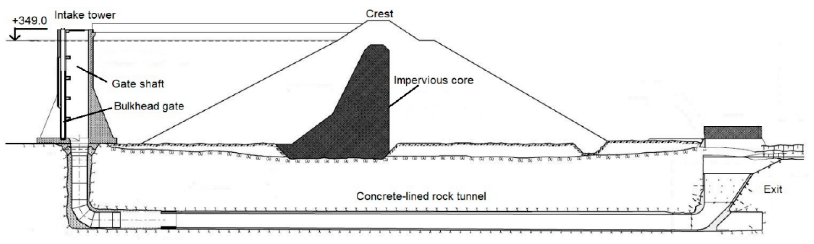
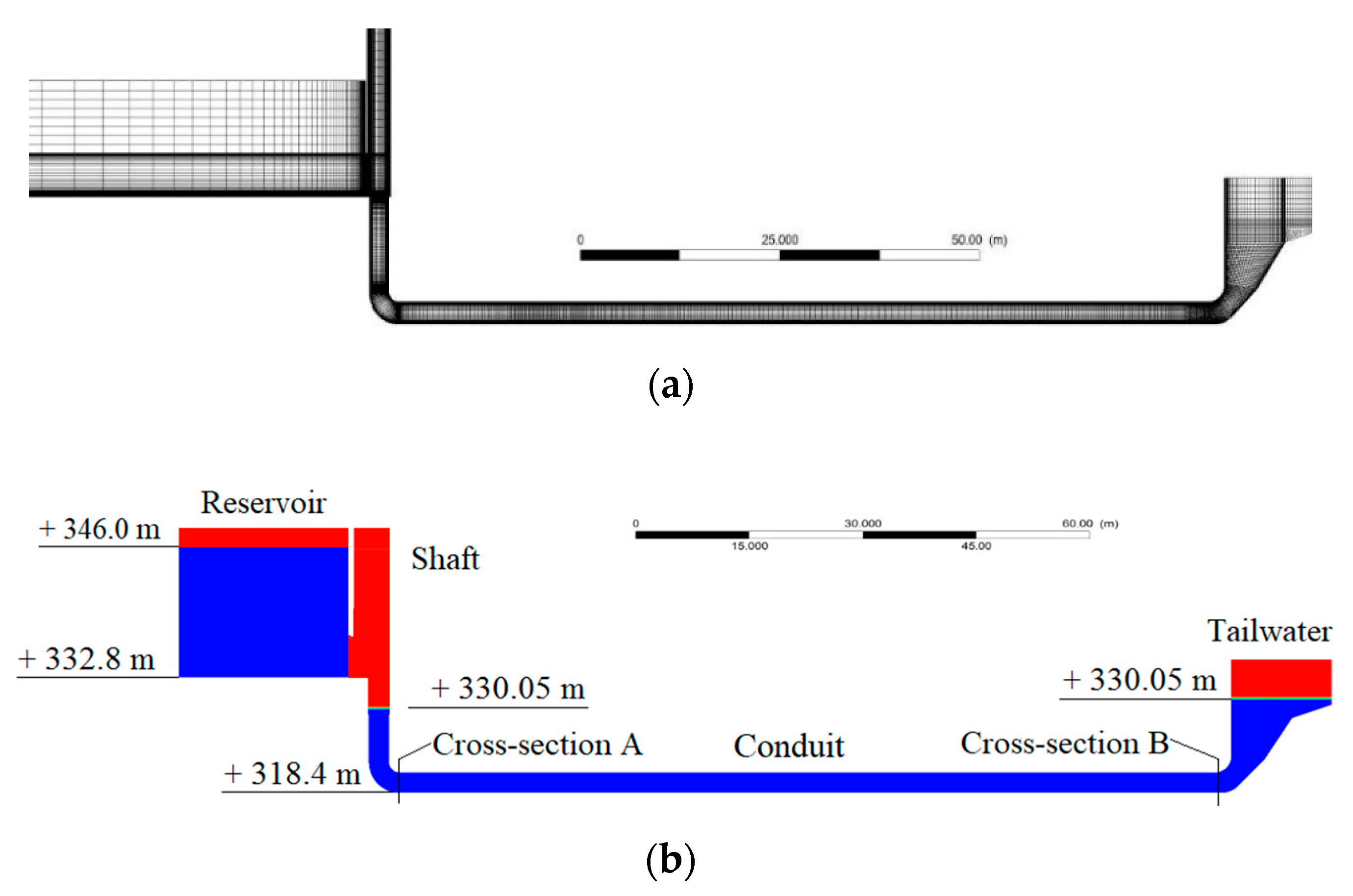
The hydropower scheme in question was commissioned in 1956. Two major embankment dams form the reservoir. Their maximum structural heights are 25 and 22 m. According to the dam safety legislation, both belong to a high-hazard class. The full reservoir water level (FRWL) is +349.00 m, at which the water-surface area is ~16 km². The power plant is of pumped-storage type and is located underground in a bedrock, with its intake in the reservoir bottom. A 6 km long rock tunnel conveys the water to the powerhouse. A long tailrace tunnel then discharges the water into the river.

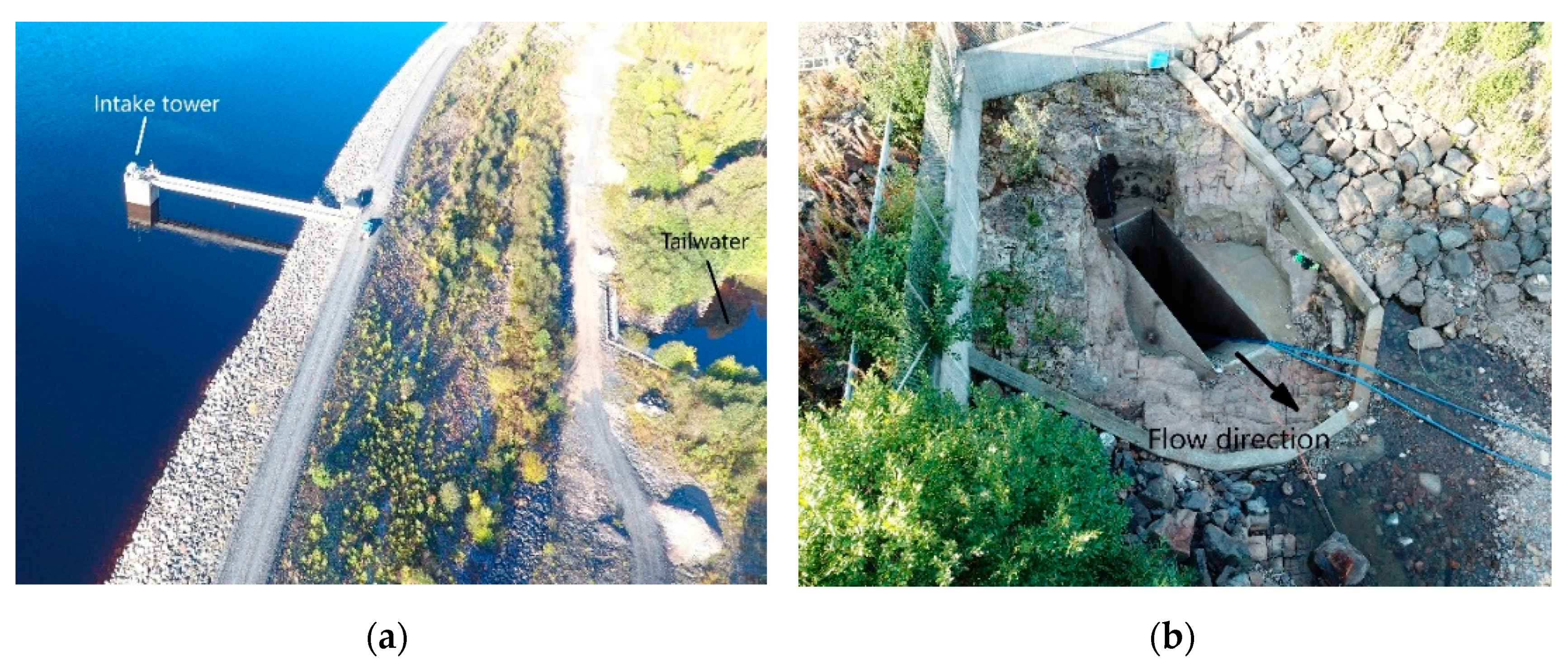
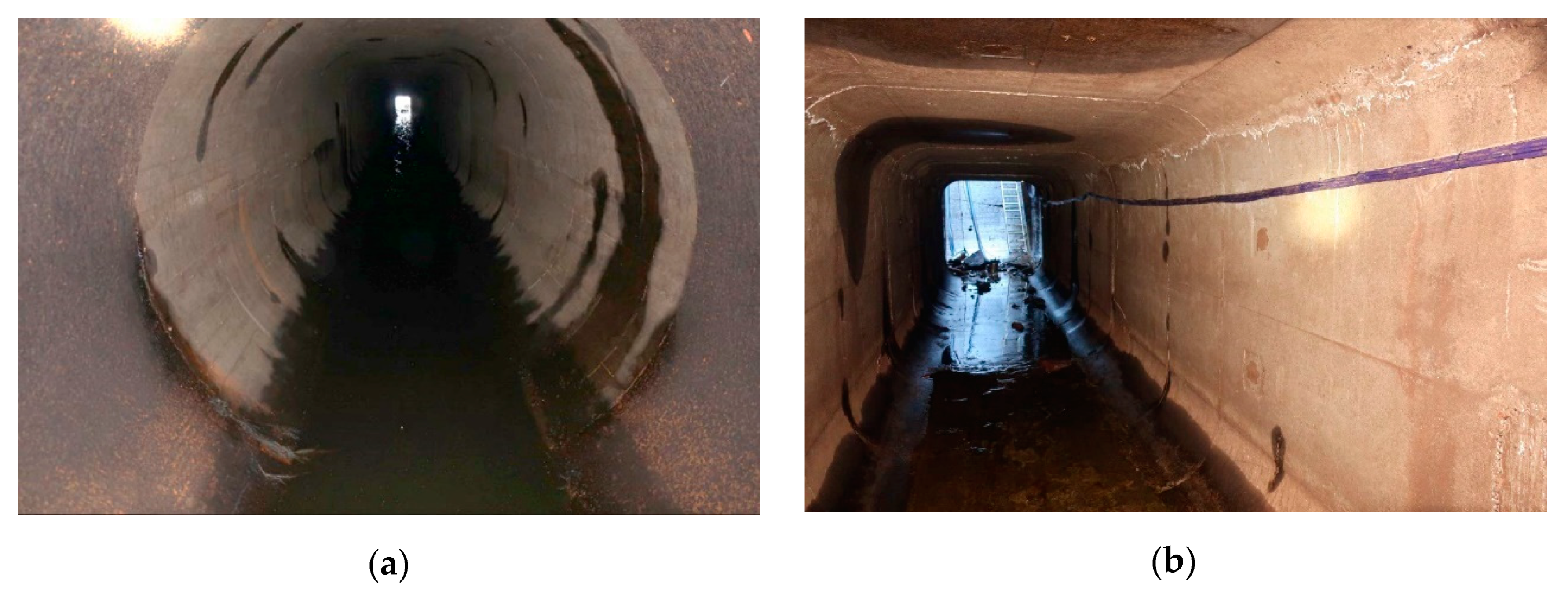
The facility has a bottom outlet for flood discharge. It is composed of an intake tower with a gate shaft, a submerged bulkhead gate, a 90° double-miter bend, a horizontal conduit, and a tailwater exit submerged even at low flow discharges. Figure 1 shows the location of the intake tower in relation to one of the embankment dams and the conduit exit when emptied of water. Figure 2 illustrates the longitudinal profile of the outlet.

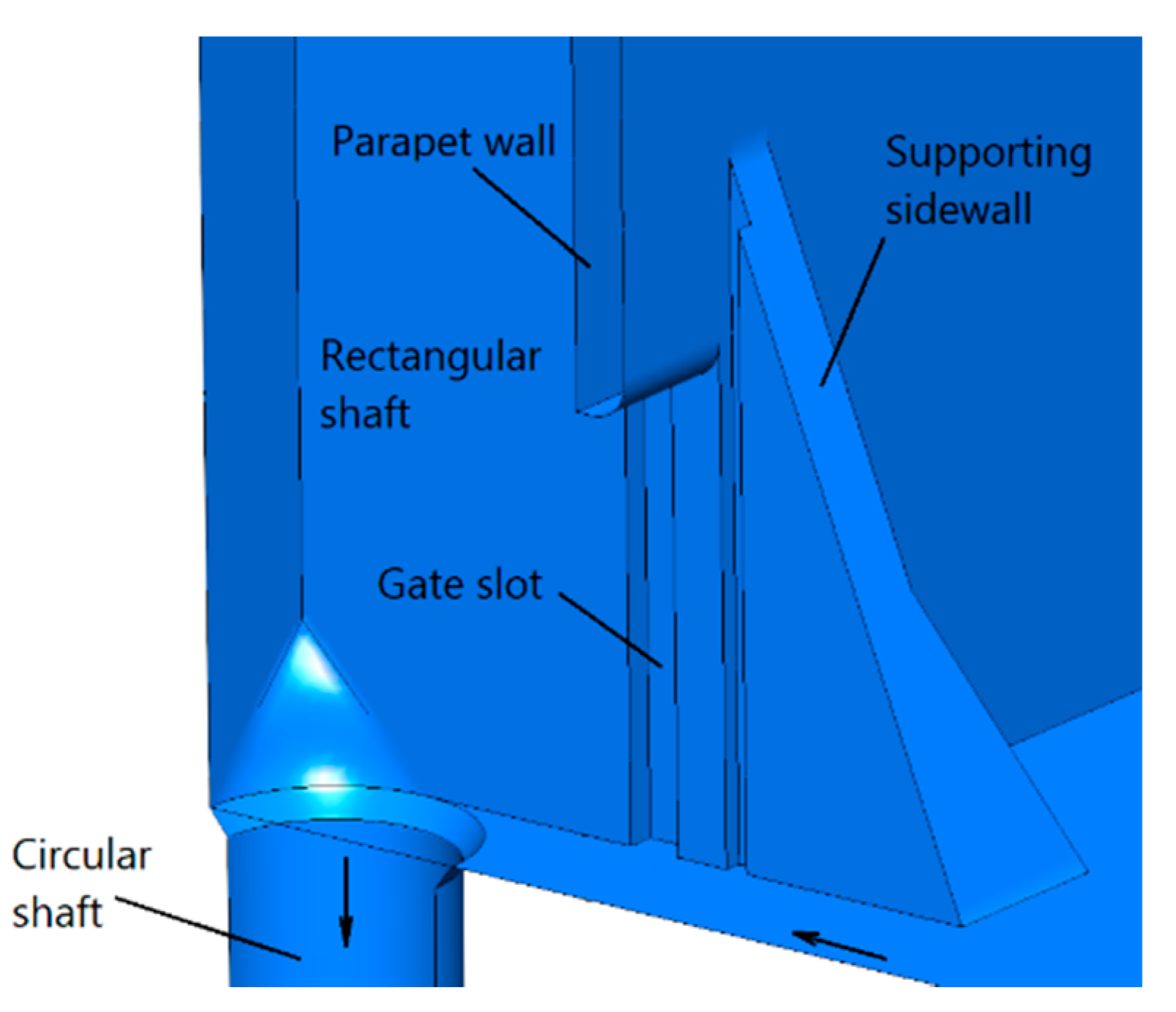
Figure 3 shows the arrangement at the gate and the transition of the gate shaft in the cross section. Upstream on each side, there exists a supporting wall. The bulkhead gate’s width is a = 3.05 m; its full opening height is h_max = 5.00 m. The gate threshold is at elevation Z₀ = +332.80 m, above which the shaft is square in the cross section (3.05 × 3.05 m, area 9.30 m²) and below which it is circular (diameter 2.55 m, area 5.11 m²). The square shaft is open to the atmosphere. From the gate threshold to the conduit bottom (elevation +321.40 m), the circular shaft is 11.40 m high.

The 90° miter bend is formed with a circular steel pipe (diameter 2.55 m), which is followed by a 13.50 m circular section of concrete lining of the same diameter (Figure 4a). The main conduit is 80.00 m long and has a rectangular cross section with four rounded corners (2.55 m in width, 2.55 m in height, area 6.32 m²) (Figure 4b). There is an 8.00 m streamlined transition between the two types of cross section; its lining is made of cast iron. The bottom elevation is the same throughout the conduit (i.e., +321.40 m, 27.60 m below the FRWL). The typical tailwater level is around +330.00 m, which is almost independent of the flow discharge. This means that the exit is submerged.

3. Field Tests and Observations

During the past decades, the use of the bottom outlet has been limited, which is mainly ascribed to safety concerns related to air entrainment and flow fluctuations. Even potential flooding and scouring of the roadways downstream play a role. The bulkhead gate is old and heavy. Due to structural deformations, significant frictional forces are also present along the gate slots. Its opening speed is dependent on several factors, such as dead weight, friction, drive system, and power supply. The gate is operated with a wire rope hoist and alternating current (AC). Limited by the hoisting capacity, the gate operates very slowly, often with a number of long stops.

The most recent field tests were performed in autumn 2018. The reservoir water level was Z₁ ≈ +346.00 m (3.00 m below the FRWL). The conduit and its exit were submerged, with the tailwater level Z₂ ≈ +330.00 m. The main purpose was to document and evaluate flow pulsations in the shaft and air blowouts at the conduit exit. Dynamic water pressures acting upon the conduit were also monitored, and the gate hoisting system was tested.

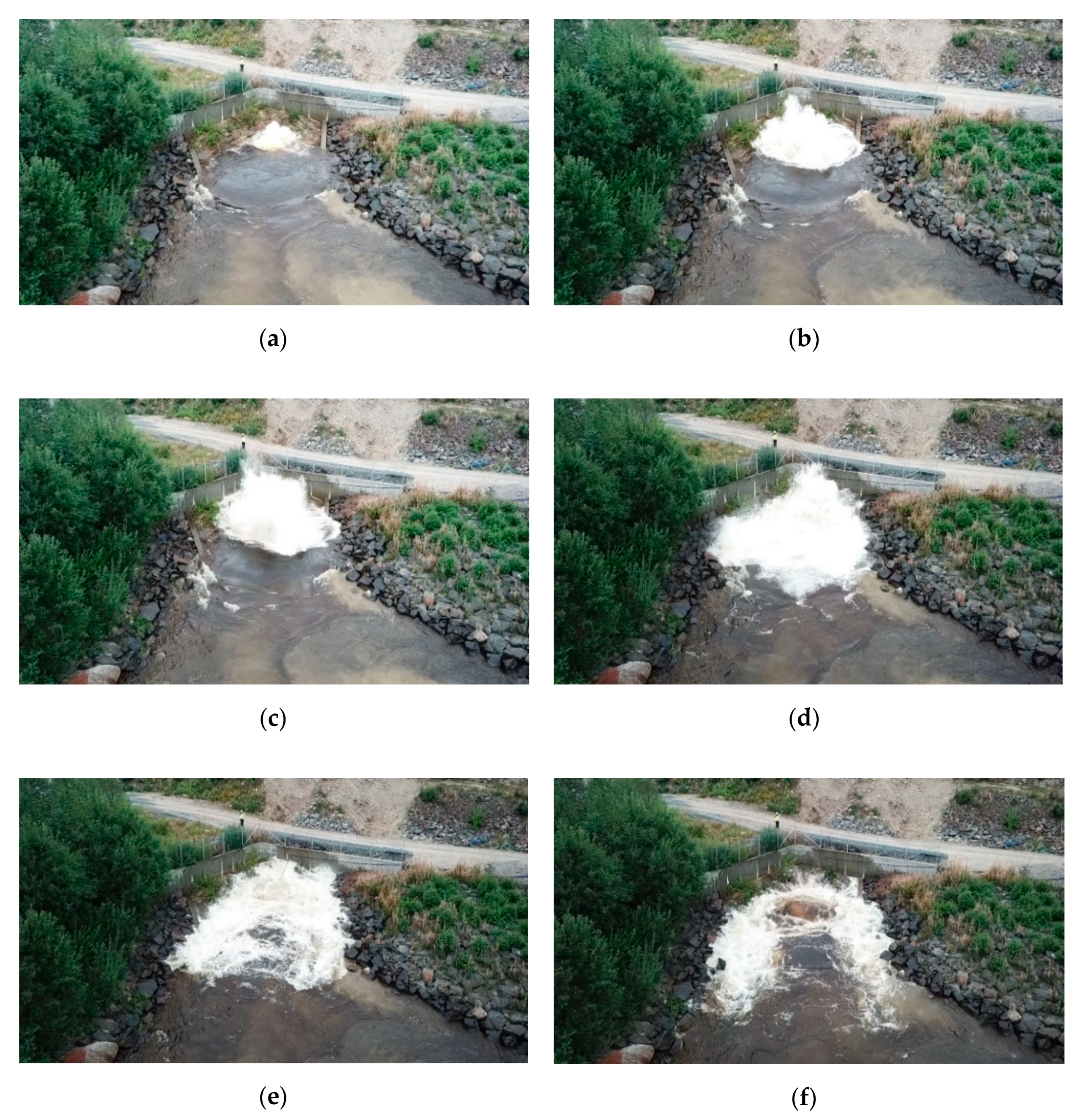
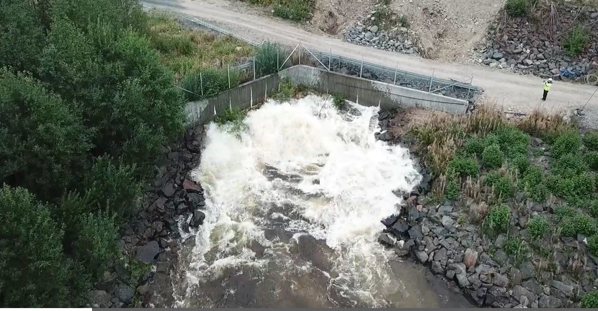
Let h (m) and Q (m³/s) denote gate-opening height and water discharge, respectively. The bulkhead gate was first opened and kept at h = 0.30 m, corresponding to Q ≈ 10 m³/s. Distinct blowouts of air and water mixture occurred at intervals at the tunnel exit. The frequency was estimated at T = 30–35 s; the blowout itself lasted 8–10 s. Figure 5 shows its sequence during the blowouts. The blowout height was not measured in the tests, but was estimated to be as high as 4.0–5.0 m. The occurrence was obviously due to the entrained air in the gate shaft, which was carried into the horizontal conduit, in which no de-aeration structure existed. This was consistent with previous observations around this gate opening.

The gate was then opened to h = 0.40 m. The discharge was estimated to be Q ≈ 14 m³/s. It was observed that this opening generated more entrained air from the shaft into the conduit, with higher, more powerful distinguishable upsurges of blowouts. At h = 0.50 m and Q ≈ 16 m³/s, it seemed that the blowouts became almost continuous and had somewhat longer durations. The resulting major upsurges, though occurring at a lower frequency, became even higher. The gate was then lifted to h = 0.80 m and Q ≈ 25 m³/s. The blowouts became lower than h ≈ 0.30 m. No distinct blowouts were observed, and the air was released almost continuously, with some minor fluctuations. The field tests were terminated at this opening. Safety concerns about both the gate operation and the discharge capacity of the downstream channel limited further discharges. There are, however, no records available with regard to its operation at large gate openings. It is therefore up to CFD modeling to demonstrate the extent of air entrainment and geysers at larger gate openings.

4. Numerical Simulations

The major concerns involved in the bottom outlet include discharge capacity, flow and pressure fluctuations, and amount of entrained air in the conduit that is eventually released as geysers. In a physical model, as known, air entrainment is not correctly reproduced due to the scale effects [34,35,36,37]. CFD simulations of the air–water flows for the outlet were therefore performed.

The two-phase model used is based on the Volume of Fluid (VOF) method, in which two fluids share a set of momentum equations, and the VOF is calculated in each cell throughout the domain [34]. Let α_w denote the fraction of water and α_a the fraction of air. For a given cell, α_w + α_a = 1.0. In the model, a surface-tracking technique is applied to a fixed Eulerian mesh. To solve free-surface turbulent flow issues with air entrainment, the VOF model is a commonly used approach. For more description of the model and its applications, one is referred to [38,39,40,41,42,43,44,45,46,47].

Figure 6a shows the computational domain with a grid (cut through the outlet center plane). The reservoir included covers an area with a 50 m radius around the intake tower. A sufficiently large area is included for the tailwater. Any CFD modeling must guarantee that its solution is grid independent. The American Society of Mechanical Engineers’ (ASME) editorial policy statement provides guidelines for the estimation of discretization errors, in which the grid convergence index (GCI) helps check the grid convergence [48,49]. To realize this, a relatively coarse grid is first generated, which is then refined twice, both globally and locally, to satisfy the criterion. The total number of cells finally adopted amounts to 960,000. A higher mesh density is given to areas around the gate, the lower part of the shaft, the upper part along the conduit, and the conduit exit where the geysers occur.

Near-wall cells should be fine enough to reasonably reproduce the boundary layer flow, which is usually judged from the dimensionless parameter of wall distance y⁺ = u_τd/υ, where υ (m²/s) = water kinematic viscosity, u_τ (m/s) = shear velocity, and d (m) = distance from the first cell’s centroid to the wall boundary. The value of y⁺ should be between 10 and 100. In the study, y⁺ is within the range 15−45. The enhanced wall function is also activated for the viscous layer.

Figure 6b shows the boundary conditions. The reservoir and tailwater levels are related to each other, set at Z₁ = +346.00 and Z₂ = +330.05 m, respectively, which are almost the same as during the field tests. In the reservoir, the domain is surrounded by water on the left, right, and upstream sides. Each side is vertically defined by two boundaries. The water part is given as a pressure inlet with hydrostatic pressure. The air part above the water surface, inclusive of the domain’s top boundary, is specified as a pressure inlet at the atmospheric pressure, allowing free two-way air flow across it. The tailrace water level is specified as a pressure outlet with the hydrostatic pressure.

It is pointed out that the aged gate is often opened for a period of half an hour, with several intermittent stops. It is numerically unaffordable to follow the opening process in the field. In the simulations, the gate is instead opened instantaneously from its closed position to a designated height. A transient flow of water and air in the waterway is thus simulated. For each time step, a fully implicit numerical scheme is used, in which the iterative convergence is checked. There is no stability criterion that governs the choice of time steps. However, it is usually set at least one order of magnitude smaller than the smallest time constant of the system. A common way to judge its choice is to count the number of iterations to a converged solution. About 5–10 iterations per time step are ideal. The iterative convergence is achieved with a decrease by at least three orders of magnitude in the normalized residuals. In terms of domain size, grid generation, turbulence model, boundary conditions, convergence, and so forth, the numerical modeling follows the best-practice guidelines for two-phase flow simulations [50,51].

5. CFD Results and Discussions

The field tests indicate that the amount of entrained air is closely dependent on the extent to which the bulkhead gate is opened. In the CFD simulations, four typical cases are examined (i.e., h = 0.45, 0.80, 3.00, and 5.00 m). Two cross sections, A and B, are chosen to monitor variations in the air–water flow. Section A is at the beginning of the horizontal conduit, and B at its end (Figure 6b). Intrinsically, the changes at section B reflect the geyser formation.

5.1. Process of Air Entrainment and Conveyance

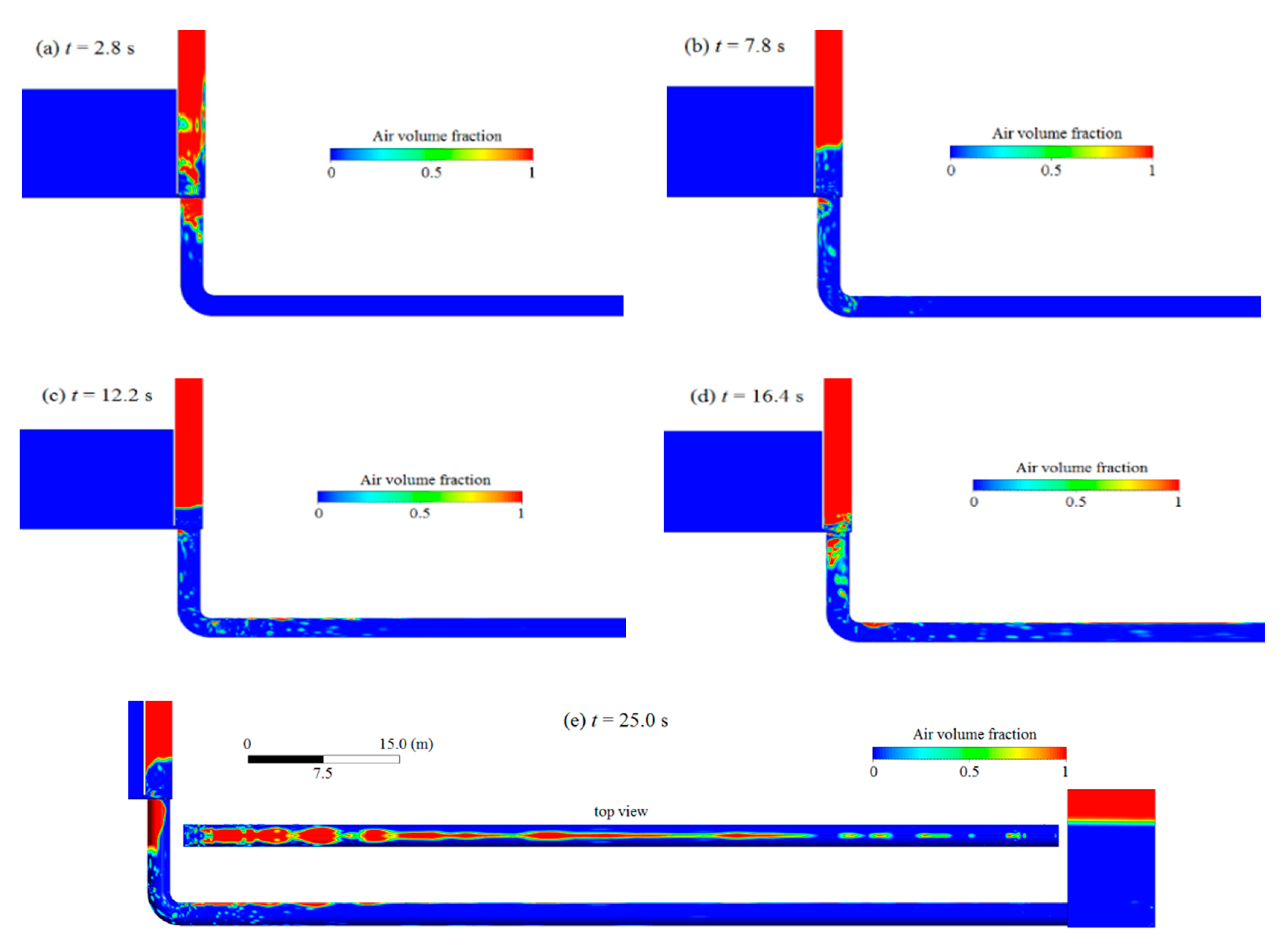
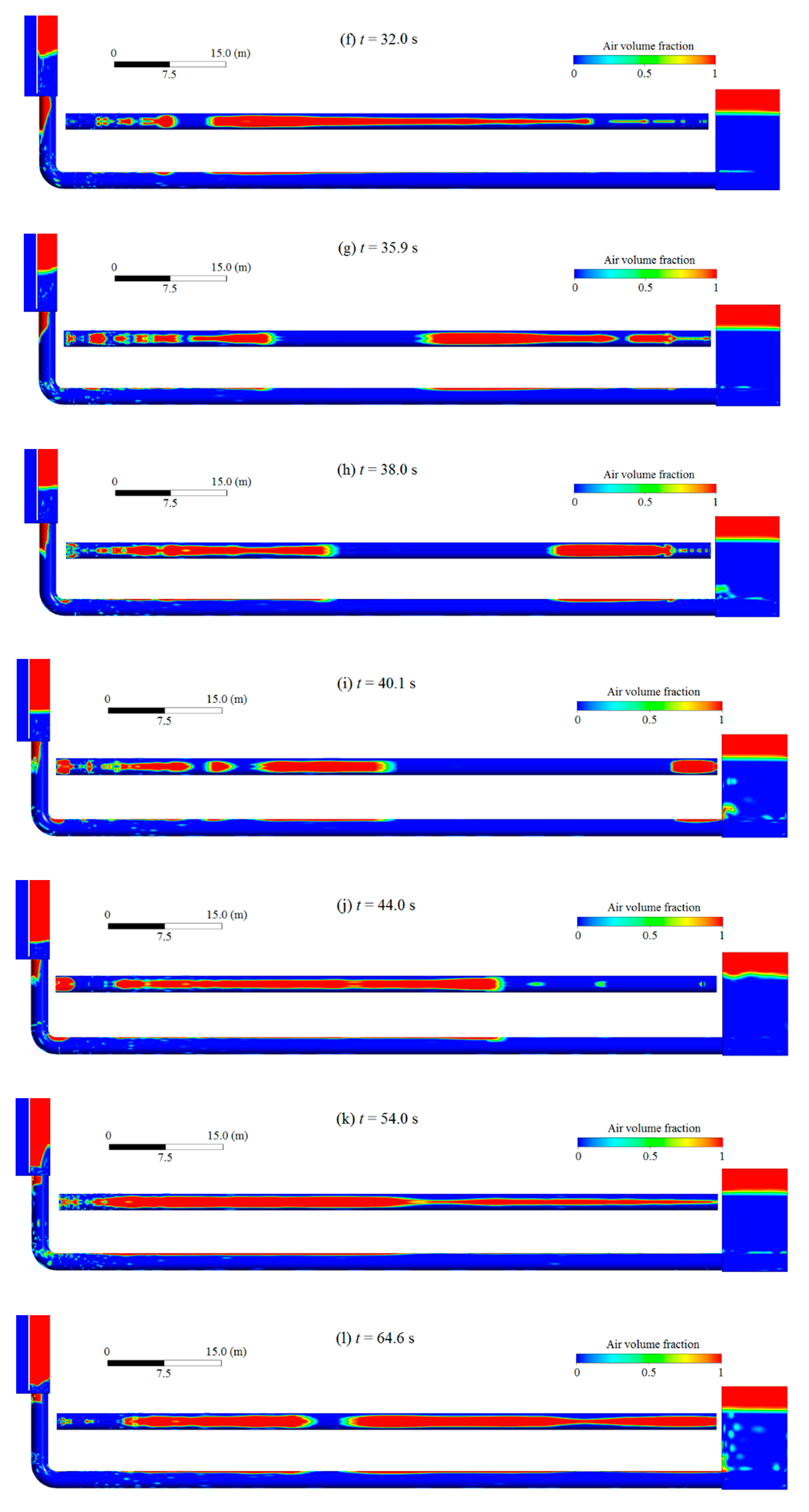
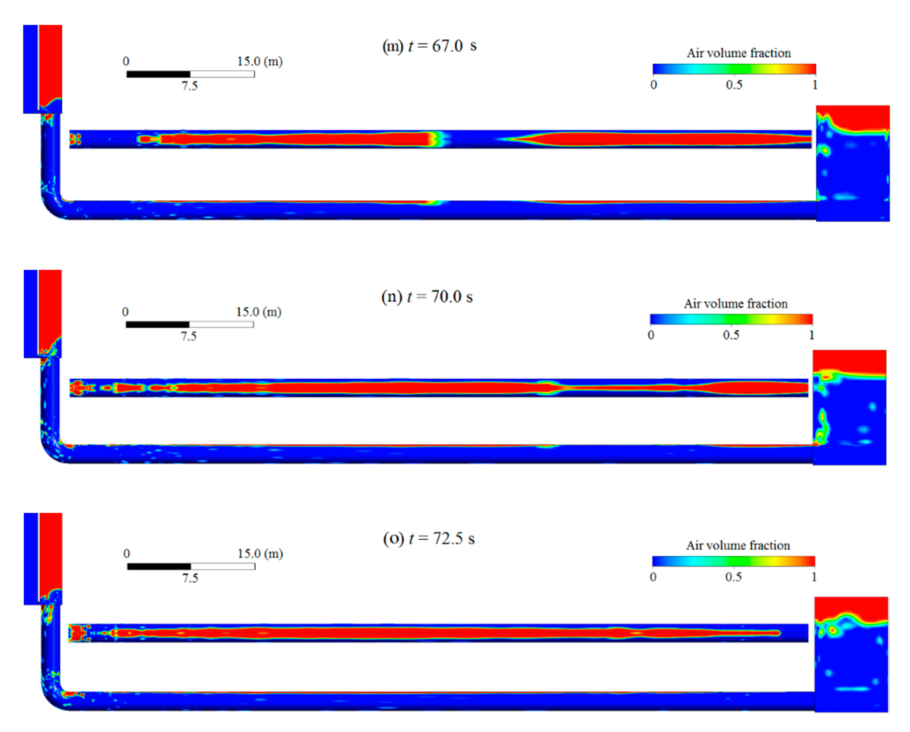
To help in understanding the air entrainment in the gate shaft, air movement into the tunnel, and blowouts at the exit, Figure 7 plots, for case h = 0.45 m, the sequential VOF pictures from simulation time t = 2.8 to 72.5 s at which the simulation ends. The water (α_w = 1.0) and air (α_a = 1.0) phases are denoted by the blue and red colors, respectively. The side views are cut through the center plane of the outlet. From t = 25.0 s (Figure 7e), even top views from above the tunnel are shown.

Before the opening of the gate, the shaft water stage is 2.75 m below the gate threshold elevation (the same as the tailwater level). At t = 0, the gate is instantaneously opened. After opening, the water jet hits the walls at the lowermost part of the rectangular shaft, resulting in sudden splashes and run-ups in the shaft. As the rectangular shaft has a larger cross-sectional area than the circular one (9.30 versus 5.11 m²), the outflow traps an air pocket of appreciable size in the latter below the threshold elevation (Figure 7a). Meanwhile, due to the sudden flow increase, the shaft water stage ascends; at the same time, part of the entrained air moves downwards with the flow and into the tunnel (Figure 7b). As the tailwater level is approximately constant, the shaft water-level rise is followed by a drop (Figure 7c). A further level drop leads to free outflow with intensive splashes and air entrainment around the gate opening; more air is conveyed into the tunnel, with the formation of air bubbles at the top (Figure 7d).

The water-level variations in the shaft are paralleled with the oscillations in a U-tube. The water level fluctuates around the gate opening and gives rise to air entrainment at intervals. At t = 25.0 s (Figure 7e), a large air pocket is formed below the outflow jet; the water stage rises again above the gate opening. However, the actual water level in the circular shaft is below the gate threshold. The increasing outflow maintains a high shaft water stage up to t ≈ 40.1 s (Figure 7i). During this period, the trapped air pocket below the outflow shrinks with time, which is due to the air entrainment and transport in the downward flow. In the conduit, small volumes of air accumulate, in motion, to form air bubbles, which in turn coalesce into long slim bubbles. Due to the flow fluctuations, long bubbles may break into short ones. The first major bubble reaches section B at t ≈ 40.1 s, whose blowout is seen in the surface water 3–4 s later (Figure 7j).

From t ≈ 50.0 s, the outflow is almost directly exposed to the atmosphere and somewhat stabilizes, the shaft water level remains at a lower elevation, and the air entrainment becomes more extensive than before. The coalescence of air bubbles leads to a second major blowout at t = 67.0–72.5 s (Figure 7m,o). With the elapse of time, the air entrainment in the shaft develops towards a relatively stable level, albeit with fluctuations.

At this gate opening (h = 0.45 m), the blowout frequency predicted by the simulations is, in an approximative way, coincident with that observed in the field tests (~30 s). The height of the blowouts, estimated at 90% air concentration in the air–water mixture, ranges between 4.2 and 4.8 m. In the field tests, no direct measurement is made. However, in relation to the reference objects on shore, image processing indicates approximately the same interval. The conduit flow is characterized by continual bubble breakup and coalescence, which is the reason for the formation of the major geysers downstream.

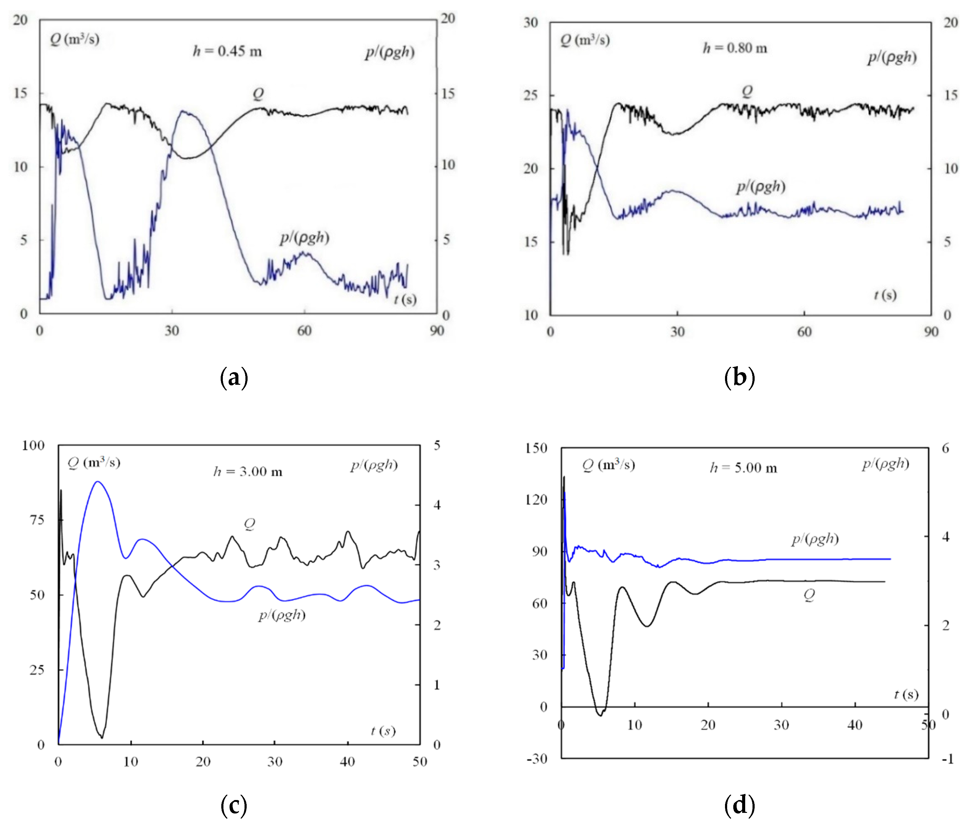
5.2. Gate Outflow Behavior

The behavior of the outflow discharge is an issue of interest for the bottom outlet, which concerns bank erosion in the open channel downstream and overtopping of the roadway crossings. For the examined cases, Figure 8 illustrates the changes of both Q and normalized flow pressure p/(ρgh), where p (Pa) = dynamic flow pressure measured at the centroid of the gate opening, ρ (kg/m³) = water density, and g (m/s²) = gravitational acceleration.

The results reveal that Q and p are closely coupled; Q varies reversely with the pressure fluctuation at the gate, especially immediately after its opening. Due to the jet impacts on the shaft walls, a water surface is indefinable in the shaft; p is therefore treated as a proxy for the shaft water-stage fluctuations.

With time, both Q and p become relatively stable and approach a quasi-steady state. However, the time it takes to do so, denoted as t₀ (s), is different and depends on h. For h = 0.45, 0.80, 3.00, and 5.00 m, t₀ ≈ 65, 40, 24, and 22 s. Obviously, less time is needed for a larger opening to reach its quasi-steady state. The outflow is submerged in all cases except for h = 0.45 m, where almost free outflow prevails. At h = 0.45 and 0.80 m, the flow exhibits small perturbations. At h = 3.00 m, the flow is characterized by moderate sustained oscillations. At h = 5.00 m, both Q and p level out.

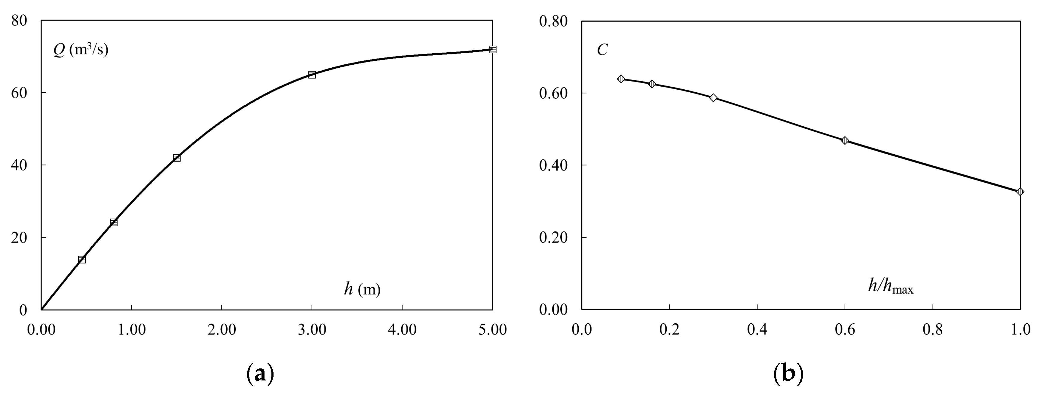
At the quasi-steady state, the outflow discharge is estimated by $Q=C{\left(2g\right)}^{0.5}ah{\left(H-0.5h\right)}^{0.5}$, where H = Z₁ − Z₀ and C = discharge coefficient in which the effect of outflow submergence in the shaft is incorporated. Figure 9 plots the Q and C results. Compared with the free orifice outflow [52], the discharge at the large openings becomes much lower, which is mainly due to the submergence effect. Note that, from h = 3.00 to 5.00 m, the Q-h curve tends to level off; the incremental discharge is only 7 m³/s. From h = 0.45 m to the full opening, C declines almost linearly with an increase in h/h_max, and the reduction in C is almost 50%. This means that the bottom outlet has much lower discharge capacity than expected.

5.3. Air–Water Interplay in the Conduit

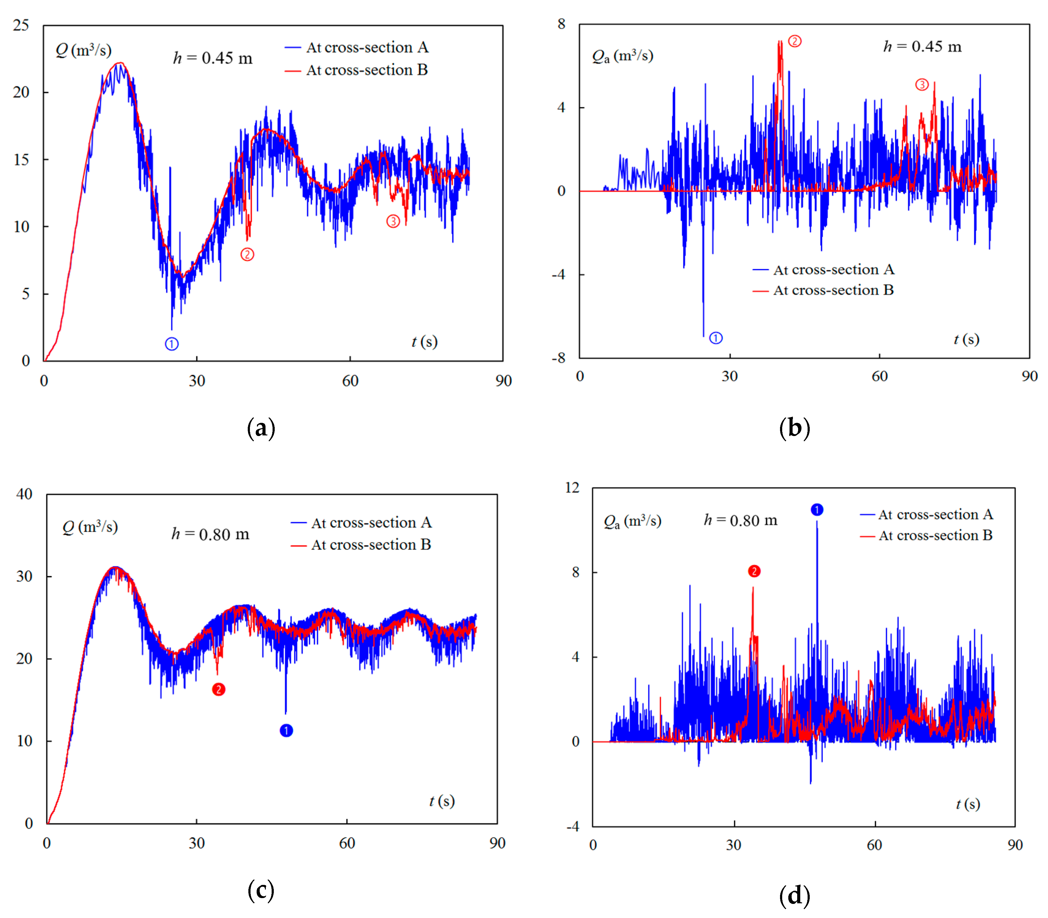
The amount of air entering the conduit is strongly dependent on the air–water mixing in the shaft and the conduit flow velocity. Let Q_a (m³/s) denote conduit air-flow rate. Figure 10 compares, for each opening, the variations of Q and Q_a at cross-sections A and B. The results (Figure 10a,c,e,g) indicate that the Q changes at cross-sections A and B follow the same pattern, which is expected.

At h = 0.45 and 0.80 m, both the flow cases are characterized by large oscillations with small add-on fluctuations. The oscillational frequency is, by estimate, near the natural frequency of the outlet, as the shaft-conduit-tailwater system can be paralleled to a U-tube. The oscillational amplitude, however, declines with time, which is ascribable to the changes in the dynamic pressure in the shaft. At h = 3.00 and 5.00 m, the conduit flow discharge exhibits only minor perturbations and approaches asymptotically a nearly constant level.

At h = 0.45 m (Figure 10b), from t = 5 s, the air enters into the conduit from section A. Up to t ≈ 19 s, there is no air present at section B. The first peak appears between t = 40 and 41 s. This means that a large air pocket blows out in the tailwater. The air movement velocity is dependent on the water flow velocity in the conduit. The second large air pocket appears at t = 66 s; its release lasts 5 s. The time interval between the first and second pockets is T = 28–29 s. At this opening, isolated geysers are evident.

At section A, negative Q_a values are evident (Figure 10b). This implies that air in the conduit moves even against the flow back into the shaft, which is due to the fluctuations in Q. At the same conduit cross section, the changes in Q and Q_a are closely related to each other. The effects of the large air pockets on Q are apparent in Figure 10a. The spikes marked by ①, ②, and ③ correspond to each other. This implies that a large Q_a leads to a low Q, which is even irrespective of the air pocket movement direction.

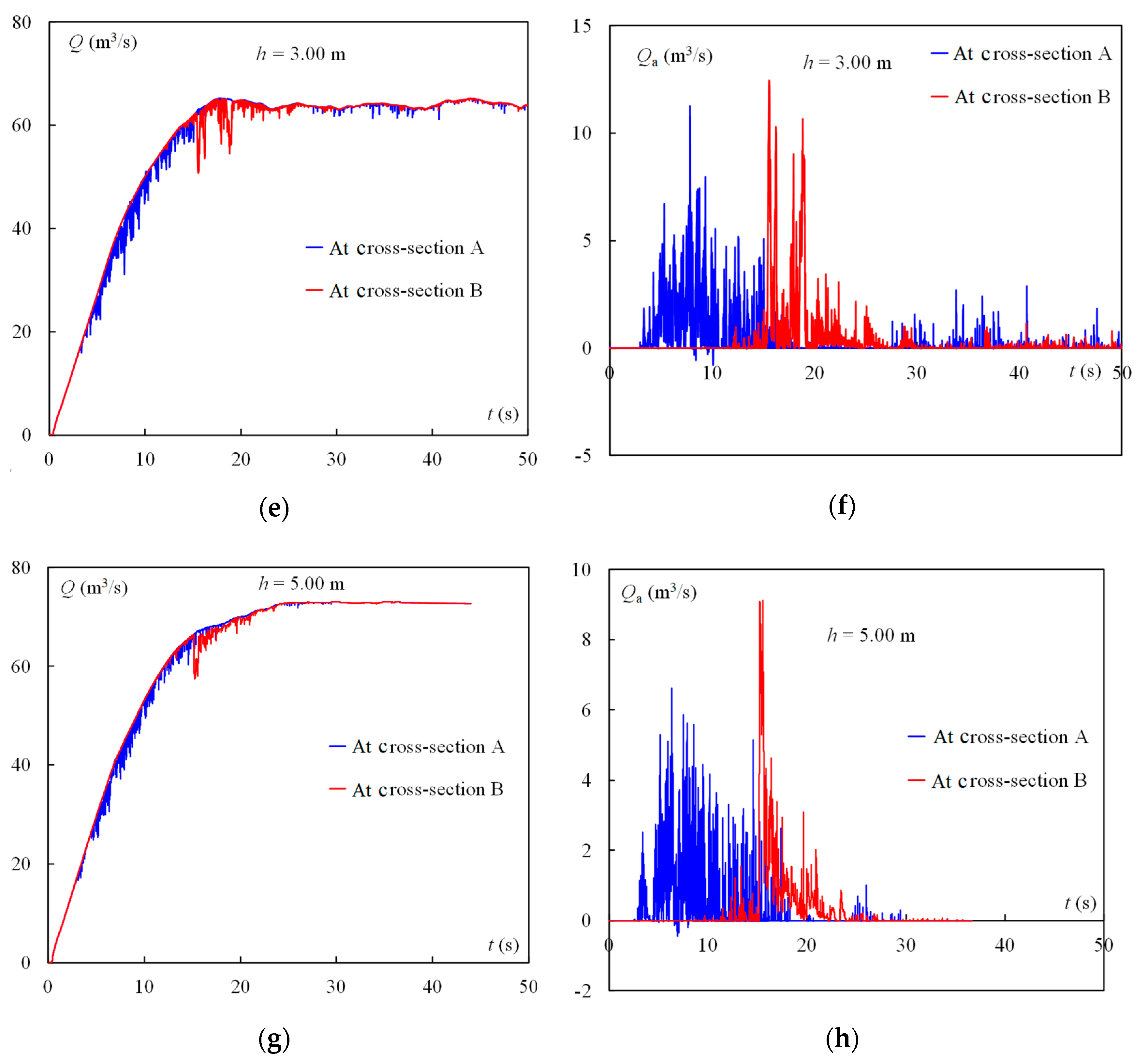
Figure 11 plots the dynamic pressure changes at sections A and B, measured at the conduit center. The marked spikes correspond to those in Figure 10b. A blowout gives rise to a sudden pressure increase of a very short duration at the conduit end. For example, the spike marked by ② lasts about 0.5 s (between t ≈ 40.5 and 41.0 s). The increment obviously depends on the air pocket volume. This means that a positive pressure wave, as a disturbance, propagates upstream. This is, however, damped with distance. It is not possible to separate this effect from the changes in the shaft.

At h = 0.80 m (Figure 10d), reverse air flows at section A are limited. It takes a shorter time than at h = 0.45 m for the air bubbles to reach section B, which is due to the higher flow velocity. The first major blowout occurs at t ≈ 33 s, followed by a series of minor ones. This is also in line with the field observation results at roughly the same opening. The spikes marked by ❶ and ❷ correspond to one another. The blowouts occur continuously, with much lower peaks than the first one and mostly at a frequency of 7–12 s. Obviously, more air is entrained than at h = 0.45 m.

At h = 3.00 and 5.00 m (Figure 10f,h), the behaviors of the trapped air in the conduit are similar. A major blowout takes place at t = 17–18 s in both cases. As the shaft water stage stabilizes at a high level, the gate opening becomes completely submerged. When the initially trapped air is carried away, air entrainment ceases to occur. At a nearly steady state, the submerged outflow amounts to 65 and 72 m³/s, respectively. At h = 5.00 m, for example, the shaft water level is at +345.1 m (i.e., only 0.9 m below the reservoir level (+346.00 m)). It can be stated that the outlet operates without air entrainment at large gate openings.

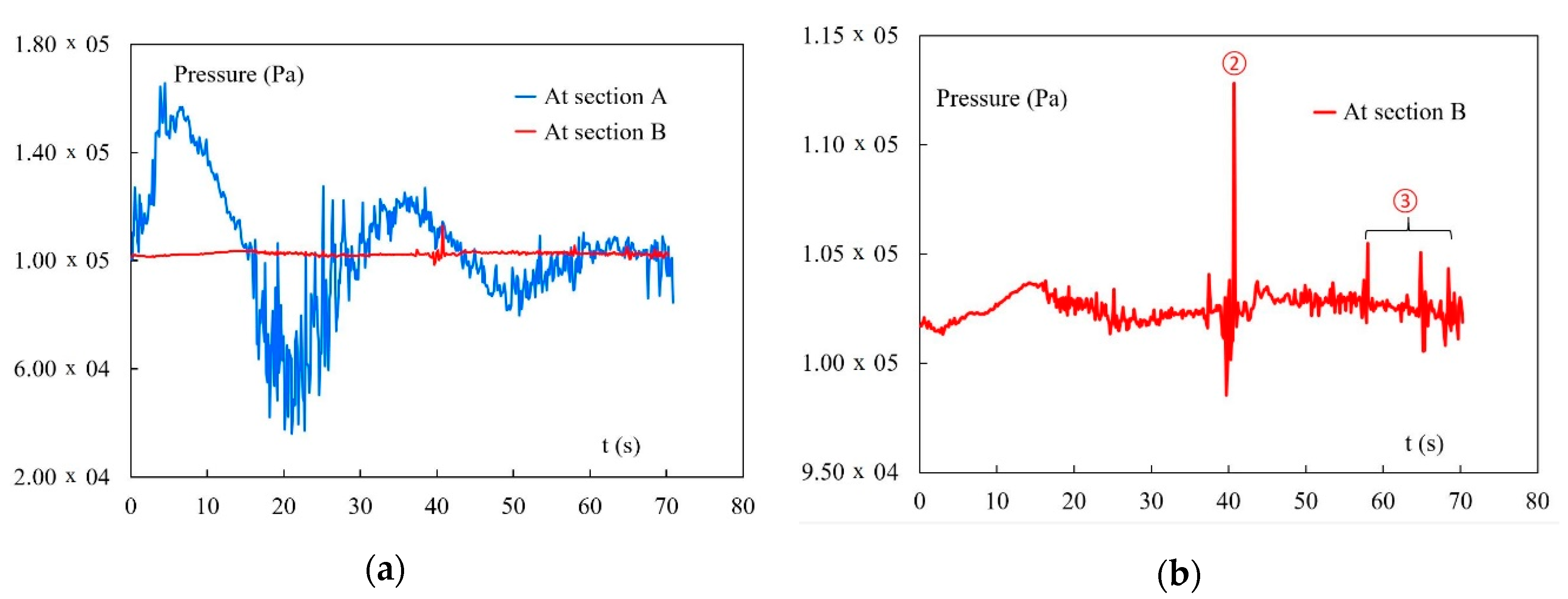
5.4. Air Volume in Conduit

The amount of air accumulated into the conduit is also a proxy for different gate openings. Air is transported down the vertical shaft into the conduit through section A and blows out through section B. Figure 12 shows the accumulation of air amount (V_a, m³) into and out of the conduit (measured at sections A and B). The difference between them is the storage in the conduit.

The horizontal conduit is approximately 93.5 m in length. At h = 0.45 and 0.80 m, the storage of air is obviously significant due to the large length. The air amount V_a increases with time almost linearly at section A. Due to the long CPU time (the wall-clock time > 1 month), the simulation terminates at t ≈ 85 s. Assuming that the simulation time is sufficiently long, the two curves should approximately run parallel to each other. At h = 3.00 and 5.00 m, when the initially entrained air is released downstream, the air entrainment stops and the two curves level off. The small difference in between is due to either air loss in the tunnel or numerical diffusion.

5.5. Discussions

In the field tests, the gate opening time is long. In the CFD, the opening is instantaneous from the closed position to a designated height. Simulating the exact field opening procedure is numerically impractical. However, it is the stabilized flow conditions that are compared and of practical interest.

Practical safety concerns limit the field gate opening to h = 0.80 m. No prototype records are available at larger openings other than this. In the CFD modeling, four openings are examined, with the expectation of comparing them with the field observations and making predictions for large openings. The reason for the opening choice in the CFD is that small openings below 1.00 m and large ones above 2.50 m are the major operation concern of the facility. The former is frequently used for flow regulations, while the latter is intended for use in flood discharges.

With the opening changing from 0.45 to 0.80 m, the shaft water level becomes somewhat higher. However, the flow rate increases and the energy of the plunging water heightens. As a result, the jet penetrates deeper in the gate shaft, implying that more air is “pushed” into the conduit. This confirms the operation restrictions at small gate openings. An opening height above half of the full opening leads to much higher shaft level, which implies that the shaft water submerges the gate, and air entrainment ceases to occur.

Under both the transient and stabilized flow conditions, the large elevation difference of the shaft water stage below the outflow governs the air entrainment. Reducing the difference would alleviate the phenomenon. Potential countermeasures, therefore, include installation of a gate at the conduit end for water prefilling or construction of a low tower in the tailwater for a high shaft water level during discharges.

6. Conclusions

The examined outlet features a typical layout with a gate shaft and a conduit running beneath the dam body. Both prototype tests and CFD modeling are performed, with the purpose of understanding the air–water flow behaviors and providing a basis for forthcoming countermeasures to guarantee safe discharge.

In the field observations, several stepwise gate openings are tested. From opening 0.30 and 0.40 to 0.50 m, the outlet is characterized by distinct geysers in the tailwater with ascending upsurge height. At the 0.80 m opening, the tailwater air release is almost continuous. Due to safety concerns, the tests are limited to openings below 1.00 m. Obviously, the air entrainment in the outlet is related the gate-opening heights, giving rise to varying degrees of water–air mixing in the shaft. However, there is no a proper method available to quantify the prototype air entrainment. In laboratory environments, a high-definition camera is usually used to monitor two-phase flows, which should be evaluated for prototype applications.

The CFD simulations of air–water flows are made, in which the bulkhead gate is instantaneously opened to a designated position. The focus is laid on gate openings below 1 meter and above half of the full opening. The results show that the entrained air in the shaft enters the conduit and leads, through breakup and coalescence, to the formation of air pockets that travel along the roof of the tunnel with the flow and finally blow out in the tailwater. At the 0.45 m opening, distinct geysers occur downstream, which agrees well with field observations in terms of both geyser frequency and upsurge height. Both exhibit almost the same frequency (~30 s). At the 0.80 m opening, the modeling points to continuous air release as evidenced in the prototype. Besides, more air is entrained from the shaft to the conduit. At the 3.00 and 5.00 m openings, the gate becomes submerged, air ceases to enter the tunnel, and water is discharged without air entrainment and blowouts.

Air entrainment is associated with the operation safety of many bottom outlets in Sweden. The entrained air and geysers give rise to undesirable flow fluctuations in the system and subsequent safety concerns. The study is intended to gain an insight into the issue and thereby provide a reference for air entrainment studies of similar bottom outlets.