Abstract
The near-shore and estuary environment is characterized by complex natural processes. A prominent feature is the wind-generated waves, which transfer energy and lead to various phenomena not observed where the hydrodynamics is dictated only by currents. Over the past several decades, numerical models have been developed to predict the wave and current state and their interactions. Most models, however, have relied on the two-model approach in which the wave model is developed independently of the current model and the two are coupled together through a separate steering module. In this study, a new wave model is developed and embedded in an existing two-dimensional (2D) depth-integrated current model, SRH-2D. The work leads to a new wave–current model based on the one-model approach. The physical processes of the new wave model are based on the latest third-generation formulation in which the spectral wave action balance equation is solved so that the spectrum shape is not pre-imposed and the non-linear effects are not parameterized. New contributions of the present study lie primarily in the numerical method adopted, which include: (a) a new operator-splitting method that allows an implicit solution of the wave action equation in the geographical space; (b) mixed finite volume and finite difference method; (c) unstructured polygonal mesh in the geographical space; and (d) a single mesh for both the wave and current models that paves the way for the use of the one-model approach. An advantage of the present model is that the propagation of waves from deep water to shallow water in near-shore and the interaction between waves and river inflows may be carried out seamlessly. Tedious interpolations and the so-called multi-model steering operation adopted by many existing models are avoided. As a result, the underlying interpolation errors and information loss due to matching between two meshes are avoided, leading to an increased computational efficiency and accuracy. The new wave model is developed and verified using a number of cases. The verified near-shore wave processes include wave shoaling, refraction, wave breaking and diffraction. The predicted model results compare well with the analytical solution or measured data for all cases.
1. Introduction
The near-shore estuary and coastal environment is characterized by complex natural processes driven by tides, waves, currents, saline water and the interactions among them [1,2]. Many people rely on coastal waters for food supply [3]. Without accurate knowledge of the near-shore bottom bathymetry, large ships would not be able to navigate onto the land safely, stifling trade routes [4]. Reclamation of coastal areas provides new land development opportunities [5]. On the other hand, the natural forces found in the coastal areas pose great threats to the surrounding communities. Every year, properties and lives are lost due to hurricanes and typhoons [6]. Land masses disappear from prolonged wave action, a process quickened when coupled with poor human intervention [7]. Over the years, the importance of the coastal environment and the need for a better understanding of it have only grown. Today, with the rising sea level [8] and shortage of natural resources following a population explosion [9], proper coastal engineering and management may be the deciding factor for many parts of the world.
From the engineering point of view, the coastal environment is unique compared to inland hydraulic systems (e.g., streams and reservoirs) in that there is constant forcing from the sea. One of the most prominent features is the wind-generated waves. Propagating from offshore, these waves can transfer energy and lead to various processes not observed where the hydrodynamics is dictated only by currents [2,10]. Waves contain energy, which is proportional to the square of the wave height. Thus, higher waves can inflict greater loads on shores and coastal structures. Much like light waves, water waves undergo such processes as diffraction (when encountering a surface-piercing object), reflection (when propagating onto a wall) and refraction (when bed elevation changes or encountering currents). Near a shore, the decreasing water depth causes the wavelength to decrease and the wave height to increase, making the waves break. Wave breaking results in wave-induced currents: longshore current, rip current and undertow. The longshore current plays an important role in coastline evolution by transporting sediment along the shore.
Historically, there have been active research efforts to model the coastal wave-related processes. Various numerical models that have been developed belong to either the process-based or behavior-based models. While the former describes the underlying physics based on the deterministic governing equations, the latter utilizes parameterized descriptions to simulate general behaviors [11]. Process-based deterministic numerical models may be divided further into several categories [12], such as conceptual models, coastline evolution models, coastal profile models and coastal area models. The coastal area models are the primary focus of the present study.
Over the past several decades, many coastal area numerical models have been developed to predict the sea state in a given environment. Fleming and Hunt [13] developed one of the earliest coastal area models, although it supported only unidirectional flows. The wave ray tracking approach was used to model wave propagation in a triangular finite element mesh. The wave-induced current was obtained with the longshore model of Longuet-Higgins [14]. Other early works include Coeffe and Pechon [15], Boer et al. [16] (COMOR model), De Vriend and Ribberink [17], Price et al. [18] (PISCES model) and Lou and Ridd [19], among others.
Some of today’s widely used wave–current models include Delft3D-SWAN [20], TELEMAC [21] and CCHE2D-COAST [22]. They provide a means to predict the sea state of a region based on the environmental inputs, and have become a vital tool for researchers, government agencies and industries alike. General reviews of these models may be found in Klingbeil et al. [23], Deng et al. [11], Lu et al. [24] and Amoudry and Souza [25]. Briefly, Delft3D-SWAN is a popular wave–current model developed by combining Delft3D—a 2D/3D finite difference current model—with the wave model SWAN [26,27]. SWAN is one of the most widely used wave models and it has been incorporated into a number of 2D and 3D current models through a two-model approach. In Delft3D, the wave-induced effects include the surface stress, radiation stress, turbulence production and boundary layer treatment. Another popular model is TELEMAC, which was, e.g., adopted by Luo et al. [28] to simulate sand transport in a tide-dominated coastal-to-estuary region in North West England. The 2D depth-integrated current model of TELEMAC-2D was coupled to the wave module TOMAWAC [21], along with a sediment transport model SISYPHE. An unstructured triangular finite element mesh was utilized for the simulation. Besides the above two, CCHE2D-COAST is also a wave–current model available to use. CCHE2D-COAST is based on the 2D depth-integrated formulation; it developed a special wave module which was coupled to the current model CCHE2D [29]. The finite element method is adopted based on the non-orthogonal quadrilateral meshes. Two algebraic turbulence closure models are supported: the approach by Longuet-Higgins [14], which relates the eddy viscosity to the distance offshore, and the Larson–Kraus model [30], in which the eddy viscosity is determined as a function of the wave orbital velocity.
The development of the wave model has been progressed independently of the current models. Today’s widely used wave models are based on the spectral method: the wave action balance equation is numerically solved. The spectral models differ primarily in the development and use of the mathematical expressions for various wave energy generation and dissipation processes. Among them are the wave generation due to wind, wave–wave interactions and wave dissipation due to bed friction, whitecapping and wave breaking. Historically, the search for a better physical process representation has led to the first-, second- or third-generation wave models.
First-generation models were developed in the 1960s and early 1970s. The validity of the first-generation formulations was extensively tested. It was found that these models were inaccurate and could lead to an order of magnitude difference in modeling wind inputs and nonlinear transfer [31]. The second-generation wave models were based on the prescribed parametric spectrum shapes, thanks to the availability of more measured wave growth data [32]. These models were reported by, e.g., Janssen [31] and WAMDI Group [33]. A major shortcoming of the second-generation models, however, was their inability to properly model waves in the presence of strong, rapidly changing winds like that of hurricanes. SWAMP [34] investigated and reported the shortcomings of the first- and second-generation wave models and suggested the need for the development of the third-generation wave models. An early third-generation model, named wave model (WAM), was developed by the WAMDI-Wave Model Development and Implementation Group in 1988 [33]. This model used the discrete interaction approximation of Hasselman et al. [35] for the nonlinear wave interactions. The wind input and source functions were formulated by Komen et al. [36]. The model replicated the observed measurements [36]. Since WAM, several other wave models were developed and reported such as WAVEWATCH by Tolman [37] and SWAN by Booij et al. [26].
All early third-generation models employed the first- or second-order finite difference schemes and were limited to the structured mesh. To model waves propagating from the deep ocean to shallow waters, more flexible meshes with multiple scales are needed. Nested structured mesh is one option to resolve the multiple spatial scales. The unstructured mesh approach, however, has been explored more extensively as it is more flexible than the nested one. The semi-Lagrangian model TOMAWAC by Benoit et al. [38] was probably the first spectral wave model using the unstructured triangular mesh. Other unstructured mesh models have been developed since. For example, Sorensen et al. [39] developed MIKE21 SW that used the unstructured cell-centered finite volume method in both geographical and spectral space. Roland et al. [40] reported the wind wave model (WWM) which employed finite element methods in geographical space. Efforts have also been reported by implementing the unstructured mesh approach into the SWAN model. For example, Hsu et al. [41] modified SWAN to utilize the finite element method in geographical space, while Qi et al. [42] implemented into SWAN the finite volume method in the geographical space. Later, SWAN was updated to include the unstructured mesh via a modified finite difference scheme [43]. Today, the third-generation wave models are widely used in wave modeling. Recent application examples include the works of Rusu [44] using SWAN and Anton et al. [45] with MIKE21 SW.
Alternative numerical methods have been explored. Efforts include the work of Yildirim and Karniadakis [46] who employed the discontinuous Galerkin methods on an unstructured mesh in geographical space and a Fourier collocation method in spectral space. The collocation method required the modification of the action balance equation to facilitate absorbing boundary conditions for frequency and required periodicity at the frequency boundaries for fast convergence of the Fourier collocation. Meixner [47] employed the discontinuous Galerkin methods in both geographical and spectral space, which allowed the utilization of the unstructured mesh in geographical space as well as adaptive, higher-order approximations in geographical and spectral space.
Following decades of model development, recent-year efforts focused primarily on the coupling of a wave model with a “third-party” numerical model. Kim et al. [48] employed two different coupled systems for simulation of the tide–surge–wave interaction during a typhoon: SWAN-ADCIRC and SELFE-WWMII. Both systems used unstructured meshes with triangular elements (SWAN and SELFE only support triangular elements). Similarly, Farhadzadeh and Gangai [49] coupled SWAN with ADCIRC to model storms in an ice-covered lake. The coupled system used a single unstructured mesh, but only with triangular elements since SWAN uses triangular elements only. On the other hand, Qu et al. [50] showed the potential for a coupling between a high-fidelity model with one designed for a much larger domain, when they coupled the 3D computational fluid dynamics model SIFUM with the ocean circulation model FVCOM. However, each model used a separate unstructured mesh and an intermediate mesh was employed in order to facilitate the solution exchange between the two. These recent examples of coupled systems all used unstructured meshes. In fact, unstructured meshes are deemed the most appropriate for wave modeling in coastal areas [51].
In this study, a new wave model is developed and embedded in the current model SRH-2D [52,53]. In terms of the physical processes, the current state of the art based on the third-generation wave modeling approaches is adopted: the governing equations largely follow the formulation adopted by SWAN to solve the wave action balance equation in which the spectrum shape is not pre-imposed and the non-linear effects are not parameterized [54]. New contributions of the present study lie primarily in the numerical methods adopted to solve the wave action balance equation. A new operator-splitting method is adopted so that each individual equation may be solved implicitly in its own space. For example, the solution of the wave action equation in the horizontal geographical space is solved simultaneously and implicitly. Discretization of the governing equation is based on a mixed use of the finite volume and finite difference methods. In particular, the finite volume method is adopted in the geographical space with the unstructured polygonal mesh. This is to conform to the mesh system adopted by SRH-2D; this way, the wave model may be embedded within SRH-2D using the one-model approach. The unstructured polygonal mesh is the most general and applicable to all mesh systems in existence. The proposed model is the first such model to our knowledge, as existing coastal models use only a special kind of mesh. An advantage of the present model is that the propagation of waves from deep water to shallow water in near-shore and the interaction between waves and river inflows can be carried out seamlessly. Tedious interpolations and the so-called multi-model steering operation adopted by existing models are avoided. The present model does not need to switch model executables during model computations. As a result, underlying interpolation errors and information loss due to solution matching between different meshes are avoided, leading to an increased computational efficiency and accuracy.
2. Governing Equations
The current model SRH-2D solves the depth-integrated, wave-averaged, 2D hydrodynamic equations, while the wave model solves the spectral wave action balance equation. The respective governing equations are presented relevant to the near-shore coastal modeling.
2.1. Current Flow
The current flow equations may be derived from the 3D Reynolds-averaged Navier–Stokes equations. Key steps include time averaging over a wave period and depth integration assuming vertical hydrostatic pressure. The final set of governing equations for the current is as follows:
In the above, t is time; x and y are the two horizontal Cartesian coordinates; h is the wave-averaged water depth; and are the total velocities in the x- and y-directions, respectively; is the bed elevation; is the seawater density; is the gravitational constant; , and represent diffusive stresses due to fluid, turbulence and dispersion; is the atmospheric pressure; and are the Coriolis forces acting in the x- and y-directions, respectively; and are the forces due to friction of the bed and wind friction on the free surface; and are the wave-induced radiation stress forces and and are the wave-generated surface roller forces. Since the present study primarily concerns the wave model, a detailed discussion of each term is omitted; readers may refer to the report of [55].
2.2. Wave Model
In deep water, wave propagation may be simulated by the balance equation of the phase-averaged wave energy (denoted as E) which describes the local energy change in the horizontal space. Such an approach is invalid in estuary and near-shore waters because it does not take into account the directional wave turning and frequency shift. The solution is to resort to the balance equation for the wave action density which is the wave energy divided by the wave angular frequency (i.e., N = E/σ) and conserved in the presence of an ambient current. The present wave model solves the following wave action balance equation:
In the above, = wave propagation direction (angle) measured counter-clockwise from the positive -axis; = wave angular frequency; = and = are group velocities in - and-directions, respectively; and = depth-integrated current velocities in - and- directions, respectively; = turning rate of the wave direction; = frequency shifting rate; and = source and sink terms for wave generation and dissipation. Equation (4) is general in that wave directional turning and frequency shift are taken into account in addition to the wave propagation in time and geographical space. The same equation was adopted by a number of the latest wave models such as SWAN. A similar but simplified steady equation was adopted in the CMS-Wave model [56].
The computation of the group velocity begins with the dispersion relation, which describes the relationship between the relative angular frequency and the wave number as
where = = wave number; = wave length; and = water depth. For a given water depth, the dispersion relation provides a unique relation between wave frequency and wave number. The group velocity is computed by
where = phase velocity of the wave.
The term is the wave propagation directional turning rate and represents the wave refraction due to depth and current changes. The turning rate is computed as
where = distance along the wave crest and = , ). The first and second terms on the right-hand side represent the depth- and current-induced refraction, respectively.
The frequency shifting may occur due to the presence of an ambient current as well as the spatial and temporal variation in depth. It may be computed by
where is the wave direction normal to the wave crest. Equation (9) shows that frequency shift is caused by three factors: time-varying water depth, waves moving across spatially varying bathymetry and waves moving with a spatially varying current.
Once the wave action is solved from Equation (4), various mean wave statistics may be obtained through integrations in the directional and frequency space. For example, the significant wave height (), defined as the mean of the highest one-third of the wave amplitudes, may be computed as
The right-hand side of the wave action balance Equation (4) contains the term which includes various physical processes leading to wave generation and dissipation. Due to the dynamic nature of the coastal environment, there is no consensus among the existing coastal models on which processes need to be taken into account and which formulations to use. In the present study, major wave generation and dissipation processes relevant to both the near-shore and deep-water environment are included, such as wave generation by wind, wave–wave interactions, wave dissipation due to whitecapping, depth-induced wave breaking, bottom friction and wave diffraction. The above processes were discussed in detail by [55]. Only the last three processes are described below as they are most relevant to near-shore coastal areas and verified in this study.
2.3. Wave Breaking
Wave breaking is a rapid wave energy dissipative process where wave energy is lost to the surface current and turbulence. In coastal waters, waves approaching the shore eventually break when the ratio formed by the wave height and water depth reaches a critical value. Depth-induced wave breaking is the dominant dissipative process in shallow waters.
Following Battjes and Janssen [57] and Yildirim [46], the depth-induced wave breaking rate of energy dissipation may be computed by
In the above, = the mean rate of energy dissipation per unit horizontal area due to wave breaking, = total wave energy in Equation (10), = a model calibration parameter (default value = 1.0), = fraction of wave breaking, = mean frequency and = maximum wave height in a given depth. The term is obtained by
where is the root-mean-square wave height amplitude, and the maximum wave height is computed as , in which is a calibration parameter (default value = 0.73). Note that Equation (13) needs to be solved iteratively in a numerical model.
2.4. Wave Diffraction
Waves approaching a coastline may diffract if there are obstacles on the way such as breakwaters. Diffraction is a phenomenon of wave turning due to amplitude change occurring around obstacles. As discussed by Holthuijsen et al. [58], diffraction is a difficult process to model within the framework of spectral (phase-averaged) wave models. Several approaches have been proposed to simulate diffraction in a wave model. For example, Hsu et al. [59] proposed an approach in which the higher-order bottom effect and ambient current effect were taken into account. Diffraction was implemented through a correction to the advection velocities in different phase spaces. In another approach, the parabolic approximation wave theory was proposed by Mase [60] and adopted by Lin et al. [56] and Sanchez et al. [61]. In this study, we adopt the diffraction modeling approach of Holthuijsen et al. [58]: the diffraction-induced wave turning rate was added to the spectral model. It is classified as the phase-decoupled diffraction approximation approach. The model aimed to provide a reasonable estimate of diffraction in relatively large-scale computations (size of the model domain is more than dozens of wave lengths for random, short-crested and non-coherent waves).
The phase-decoupled diffraction approach computes the diffraction parameter as follows:
In the above, is the phase velocity computed by Equation (7). Once the diffraction parameter is computed, the three turning rates in the wave balance equation are modified to include the diffraction effect. The group velocity () is replaced by , while the frequency shift rate and directional turning rate are modified as follows in the Cartesian coordinate system:
The diffraction parameter in (14) is computed using the second-order discretization of the term . The above diffraction approach was implemented in the SWAN model; both Holthuijsen et al. [58] and Enet et al. [62] found that diffraction produced ‘‘wiggles’’ of the wave fields in the geographical space. Wave energy () had to be smoothed using a convolution filter; it was found that six times of filtering was the smallest smooth value to maintain the model stability. A similar smoothing is also implemented in the present study, although found unnecessary.
2.5. Dissipation due to Bottom Friction
The bed friction is insignificant in deep water. In shallow water, however, the bed surface may induce significant friction, leading to wave dissipation. The bed friction term is expressed as [63]
where = a calibration parameter related to the bottom bed friction. The parameter has a default value of 0.038 [46].
2.6. Initial and Boundary Conditions
The initial and boundary conditions of the wave action balance equation are needed to solve the governing equation. At the beginning of the computation, the wave action density is needed in geographical space and frequency and direction spaces. A zero wave field may be applied over the entire model domain, or the wave field is assumed constant in the geographical space which is the same as the incoming waves from offshore.
Different boundary conditions may be applied on the model boundaries. On the shoreline and other wall boundaries, all incoming wave energy is absorbed. Waves are allowed to leave the model domain freely. On the cross-shore boundaries, the symmetry condition is imposed. At both ends of the direction and frequency space, the fully absorbing condition is adopted so that the energy can propagate freely across the boundaries.
At the offshore boundary, incident waves in the form of a 2D energy spectrum are specified. Key incident wave parameters include the wave height, direction and period. The most commonly used representative wave height is the significant wave height () which is the average height of the highest one-third of the waves. The significant period () is often used which is the average period of the highest one-third of the waves in the record. Mean or peak period (or frequency) may also be used.
Analytical spectra have been developed and verified with the field data that may be used to specify an incoming wave spectrum. The 2D energy spectrum is specified by giving two 1D distribution functions:
Established wave spectra are available for the directional distribution function () and the frequency distribution function ().
In this study, the directional spreading function of Mitsuyasu et al. [64] is used, which is based on extensive measurements of directional wave spectra. The function is often called the cos2s method and written as
In the above, is the gamma function and the parameter has the property that higher values give a more widely spread directional spectrum.
The frequency spectrum may be specified by several ways such as the Gaussian, JONSWAP or user-specified discrete spectra. The JONSWAP spectrum was based on the data of a Joint North Sea Wave Project operated by laboratories from four countries [32]. Wave and wind measurements were taken with a sufficient wind duration to produce a deep water fetch-limited energy spectrum. It is suitable when the offshore boundary is located in deep waters (e.g., > 45 m). The JONSWAP spectrum was discussed in Lai and Kim [55].
3. Numerical Method
The numerical method of the current model SRH-2D was documented by Lai [52] and Lai [53]; readers may refer to these references. The solution of the wave action balance equation is described below as it is a new contribution in the present study.
The mixed finite volume and finite difference method is adopted: the finite volume discretization is adopted in the geographical space, while the finite difference scheme is adopted in the directional and frequency space. The semi-implicit scheme is adopted in time: the wave action balance equation is first split into three equations using the operator-splitting method, and each equation is then solved using the implicit time discretization. In general, a larger time step may be used with the implicit scheme than the explicit one. The implicit scheme tends to be more stable and robust for engineering applications.
3.1. The Operator-Splitting Technique
The wave action density propagates in five dimensions (, , , and ). A fully implicit method would be computationally too intensive. Thus, the operator-splitting method similar to Hsu et al. [41] is adopted as follows:
In the above, , , and are at different fractional time levels, with being the results at time tn and tn + ( = time step). Our approach deviates from Hsu et al. [41] on how the geographical space equation is split and solved. Our approach is to solve the complete equation in the geographical space (x and y space) along with the source/sink terms included implicitly. Hsu et al. [41] split the third equation further into three more equations. In addition, our discretization approach is based on the unstructured polygonal mesh in the geographical space—the most flexible mesh in use. The operator-splitting technique brings two major advantages: an optimum numerical algorithm that may be adopted for each equation and the facilitation that is afforded for monitoring and studying the wave processes in a particular space.
3.2. Solution in the Frequency Space
In the frequency space, steep gradients may pose a problem to the numerical solution in that a large truncation error may lead to numerical oscillations. For increased stability, the flux-corrected transport algorithm of Boris and Book [65] is adopted, which prevents the steep gradient problem by enforcing continuity and positivity of the action density [41].
The frequency space is uniformly discretized in terms of between the user-specified minimum and maximum frequency. The governing equation is then discretized using the finite difference method. The discretization consists of three stages: the low-order transport stage, the anti-diffusion stage and the corrected transport stage.
The wave action density at the low-order transport stage is determined in terms of the fluxes , which are computed using the first-order upwind scheme:
In the anti-diffusion stage, the high-order fluxes and the correcting fluxes are obtained from the following relations:
The correction terms are then computed from
where
In the third and final step, the new wave action density is computed by
3.3. Solution in the Directional Space
In the directional space, an implicit finite difference scheme is adopted. The directional space is uniformly divided into a user-specified number of points between the minimum and maximum angles. At each angle point (j), the governing equation may be discretized as
In the above, the weight parameter ranges from 0 to 1 and controls the time discretization order (0 for a fully explicit scheme and 1 for a fully implicit scheme). The central difference scheme is adopted in the discretization of the flux term. In the present study, = 1 is used. The above equation may be easily put into a matrix form that is solved using a tri-diagonal matrix inversion solver.
3.4. Solution in the Geographical Space
In the geographical space, the wave action balance equation is of the convection–diffusion type in a 2D form and the finite volume method is used for its discretization. First, a 2D solution domain in space is used to represent the area of interest and a network of mesh cells is generated to cover the model domain so that the equation may be discretized on the mesh. In this study, the same mesh is used for both the current and wave models so that the one-model approach may be implemented. This means the most general unstructured polygonal mesh is used to solve the wave equation. In this study, only a mixture of triangles (TRIA) and quadrilaterals (QUAD) are demonstrated with cases.
The geographical equation is discretized using the finite volume approach, following the work of Lai [53]. The dependent variables are stored at the centroid of a polygonal cell. The governing equation is integrated over a polygon using the Gauss theorem. For the purpose, the wave action balance equation may be rewritten in a general form as
The integration of the above over a polygon P shown in Figure 1 leads to
where A is the mesh cell area, is the speed normal to the polygonal side (e.g., P1P2 in Figure 1) and at the side center C, is the polygon side unit normal vector and is the polygon side distance vector (e.g., P1 to P2). Subscript C denotes a value at the center of a side and superscript n+1 denotes the time level. In the remaining discussion, superscript n+1 will be dropped for ease of notation. Time discretization follows the Euler implicit scheme.
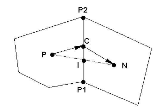
Figure 1.
Schematic illustrating a polygon mesh cell (P) and its neighbor cell (N).
Calculation of a variable, say N, at the center (C) of a side is needed. As shown in Figure 1, point I is first defined as the intercept point between line PN and P1P2. A second-order interpolation gives
in which and . may be used to approximate the value at the center C for most variables. Another approach may be used to compute the wave speed in which a damped scheme is derived by blending the first-order upwind scheme with the second-order central difference scheme; that is,
where is the second-order interpolation scheme. In the above expression, d defines the amount of damping used. In most applications, d = 0.2~0.3 is used.
The source/sink terms in the wave action equation can be excessively large and their impact is treated implicitly as much as possible. In the present implementation, wave energy generation terms are treated explicitly, while most dissipation terms are treated implicitly in a linear fashion, as follows:
The final discretized governing equation for cell P may be organized as the following linear equation:
where “nb” refers to all neighbor polygons surrounding P. The coefficients in this equation are
The linear equation system (41) is solved using the conjugate gradient squared solver with the Incomplete Lower-Upper (ILU) preconditioning [66].
3.5. Coupling Procedure
In this study, the one-model approach with a single mesh is used for both the current and wave models and data exchanges between the two are achieved as soon as the data are available. Only the quasi-steady coupling method is implemented: the current flow is assumed to be steady within a user-specified time period and computed first. The current velocity and water depth are then passed onto the wave model to solve the wave action balance equation in an unsteady manner with a time step. Under the quasi-steady coupling, the impacts of the current on the wave characteristics are simulated while the wave-to-current feedback is not. The quasi-steady coupling is applied in all verification cases presented as the cases indeed have no feedback from waves to currents.
The wave model developed has undergone an extensive verification modeling study; cases have been selected to verify individual wave processes that have either analytical or measurement data. In the following, the model capability to simulate wave shoaling, wave refraction, wave breaking and wave diffraction is reported.
4. Wave Shoaling and Refraction
Six cases are chosen to verify the wave shoaling and refraction processes. All six cases have analytical solutions for comparison and have been widely used for wave model verification studies [26,41,46,47,67].
All cases use the same geographical horizontal model domain: a 4 by 4 km square. Although these cases may be simulated using simply a quadrilateral mesh, the mixed quadrilateral-triangular mesh is used instead so that the polygonal mesh implementation may be verified with the model. The model domain and the mixed mesh with a total of 4744 cells are shown in Figure 2.
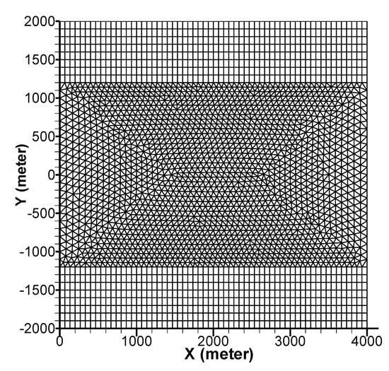
Figure 2.
Model domain and the mixed mesh for the simulation.
The boundary conditions are as follows. All six cases have the same incoming wave: entering the model domain on the left boundary (X = 0) and leaving the right boundary (X = 4000). The incoming waves have a Gaussian distribution for the energy density in the frequency space. The mean wave frequency is 0.1 Hz with a standard deviation of 0.01 Hz—almost a harmonic wave. In the directional space, the distribution follows the cos2s function with s = 250; the user-given mean angle and half-angle width are specified for each case. The incident wave has a significant wave height of 1.0 m.
4.1. Current-Induced Shoaling
Cases 1 and 2 are used to verify that the wave model is capable of reproducing the current-induced shoaling while the waves propagate in a constant-depth zone. The shoaling herein refers to the change of wave height (or energy). The model domain has a flat bottom with deep water (10 km). The incoming wave propagates along the x-axis and encounters a linearly increasing velocity field. The current velocity of case 1 is opposite to the wave propagation direction, while case 2 is along the wave propagation. The current velocity magnitude linearly increases from 0 on the left boundary to 2.0 m/s on the right. Figure 3 graphically depicts the two cases.
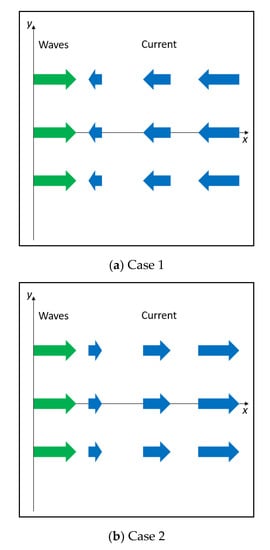
Figure 3.
Schematic of wave propagation and current velocity directions for cases 1 and 2.
Wave shoaling of the two cases is induced by the group velocity change and frequency shift. The absolute group velocity is altered by the current flow, so the waves slow down for case 1 and speed up for case 2. This causes the wave height increase or decrease. The frequency shift (non-zero ) may occur due to a change of water depth or a spatially varying current velocity (presence of velocity strain rate). In the current two cases, only the non-zero velocity strain rate is responsible for the frequency shift. The wave energy transfer in the frequency space leads to changes in the mean frequency and the significant wave height. Both cases have zero turning rate in the directional space.
The simulation adopts the following model inputs: 21 points in the directional space between −30° and 30° and 41 points in the frequency space from 0.04 to 0.25 Hz. The simulated significant wave height at steady state is compared with the analytical solution derived from the linear wave theory. The analytical solution was presented by Philips [68] and Mei et al. [69].
The predicted steady-state results of the significant wave height for the two cases are compared with the analytical solutions in Figure 4. Good agreement is obtained. When the wave propagates against the current (case 1), the wave height increases; when the wave follows the current (case 2), the wave height decreases. The effect on the wave height is more prominent in the opposing than the following case. Adam [67] pointed out that the above analytical solution has a theoretical limit at c = −2U when the wave height becomes infinite. In real life, the linear solution is invalid when the phase velocity is close to the limit; various non-linear processes will occur before the limit such as wave breaking.
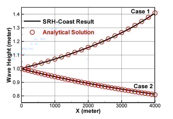
Figure 4.
The predicted significant wave height and the analytical solution for cases 1 and 2.
4.2. Current-Induced Refraction
Two additional cases (3 and 4) are selected to verify the ability to reproduce the current-induced refraction. Refraction refers to the turning of wave propagation in the directional space. Refraction may be induced by spatially varying the velocity or water depth. Only the velocity strain rate is present for cases 3 and 4. Part of the wave energy is swept away along the direction of the current. In addition, two other mechanisms lead to small wave height changes: the action of the current velocity and the velocity strain rate. The current velocity modifies the group velocity and the velocity strain rate initiates the wave energy transfer.
The model domain has a flat bottom with deep water (10 km). The current velocity field is prescribed as follows: the x velocity is zero everywhere, while the y velocity changes linearly from 0 on the left boundary to −2.0 m/s on the right boundary. For case 3, the incoming wave enters the left boundary at an angle of ; case 4 has the incident wave angle of . The schematic of the two cases is depicted in Figure 5.
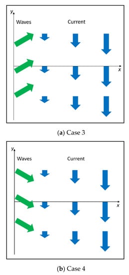
Figure 5.
Schematic of wave propagation and current velocity directions for cases 3 and 4.
The simulation adopts the following model inputs: 41 points in the angle space covering a half-angle of 30° and 41 points in the frequency space with a frequency range of 0.04 to 0.25 Hz. The analytical solutions of the wave height and wave propagation angle for the two cases are available and were discussed by Longuet-Higgins and Steward [70].
The predicted significant wave height and mean wave propagation angle are compared with the analytical solutions in Figure 6. For case 3, part of the wave propagation is against the current, so the wave height grows; for case 4, wave propagation follows the current, so the wave height decreases. In both cases, the waves are pushed towards the current direction, causing their mean direction to change towards the current. The numerical model reproduces the analytical solutions reasonably well.
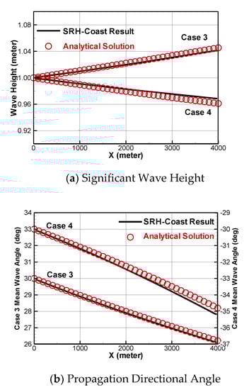
Figure 6.
Predicted significant wave height and wave angle in comparison with the analytical solution for cases 3 and 4.
4.3. Depth-Induced Shoaling and Refraction
The depth-induced shoaling and refraction are verified using two additional cases (5 and 6). In the previous four cases, a constant deep-water depth is specified with a spatially varying current velocity field. For cases 5 and 6, the bed elevation (or water depth) varies spatially, without the current velocity.
The same model domain and the meshes as the previous four cases are used except that the bottom bed elevation varies linearly from −20 on the left boundary to −0.5 m on the right. The cases represent a typical plane beach front. A long wave enters the domain through the left boundary which has a water depth of 20 m; the wave propagates towards the shallow right boundary with a depth of 0.5 m. In case 5, the wave is along the x-axis, perpendicular to the left boundary (angle = 0°); in case 6, the wave is along the 30° angle. The two cases are depicted in Figure 7.
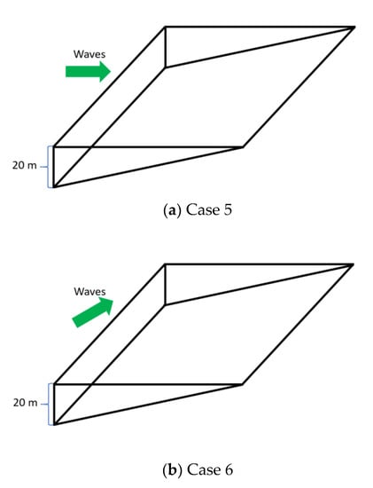
Figure 7.
Schematic of test cases 5 and 6 for the wave propagation over an inclined flat bottom and in a quiescent current field.
For both cases, the waves move towards the shallower area and decrease their speed. The bed slope causes the wavelength to decrease and the wave height to increase (shoaling). For case 6, a component of the wave direction is along the shoreline with varying water depth along its normal direction. This causes different parts of the wave to travel with different speeds and leads to the turning of the wave direction towards the shallower area (refraction). Both cases have zero frequency shift as the current velocity is zero, so the frequency space discretization is unimportant. The analytical solutions of the two cases may be derived from the linear wave theory according to Snel’s law as presented by Adam [67].
The simulation has the following model inputs: 21 points in the directional space with a half angle-width of ; the number of points in the frequency space is unimportant as there is no frequency shift. The simulation with a different number of frequency points has confirmed this: results do not change when 1 or 21 points are used in the frequency space.
The simulated results are compared with the analytical solutions in Figure 8 for the two cases. The model results compare well with the analytical results. As the waves propagate towards the shallower area, the significant wave height increases. Most of the increase happens in the last few meters near the right shore when the depth approaches 0.5 m. This suggests that the mesh point density should be finer in the shallow area for a coastal simulation. If the depth would be allowed to reach zero, the group speed of the wave would approach zero and the wave height would become infinite. This is the reason the minimum depth is set to 0.5 m on the right boundary in the simulation. The infinite wave height is simply a consequence of the linear wave approximation. In reality, the wave energy would be dissipated by non-linear processes such as wave breaking before the wave speed is near zero.
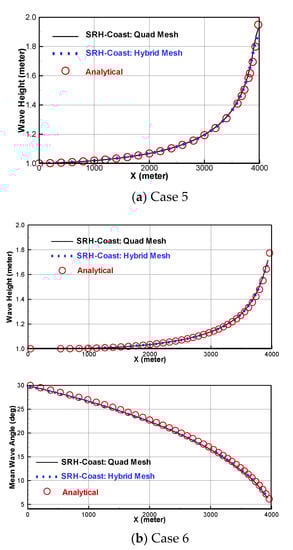
Figure 8.
The significant wave height and mean wave propagation angle and comparison with analytical solutions.
Depth-induced refraction for case 6 is caused by the phase speed changes which in turn are due to depth variations along the crest of a wave. The rate of refraction is controlled by the gradients of the depth. According to the linear theory, when the depth and phase velocity become zero, the mean direction becomes perpendicular to the shore, regardless of the incident mean direction in deep water. In other words, the waves would almost always travel normal towards the coastal shore where the water depth is ultimately zero.
5. Wave Breaking
For typical near-shore applications, waves propagate in shallow waters over a spatially varying bed elevation. As the waves approach the shoreline, the wave height increases initially due to the interactions with the bed; waves, however, break down eventually. Waves approaching coastlines may interact with the bed in many ways: relevant processes include, e.g., bottom friction, depth-induced breaking, percolation, wave-induced bottom motion and scattering [71]. Under shallow-water circumstances, however, depth-induced wave breaking is the dominant wave dissipation mechanism [46] which is the subject of model verification here.
A verification case is selected to test the dissipation due to the depth-induced wave breaking. The laboratory experiment carried out by Battjes and Janssen [57], as depicted in Figure 9, is simulated. The case was numerically studied by Adam [67], Booij et al. [26] and Yildirim [46].
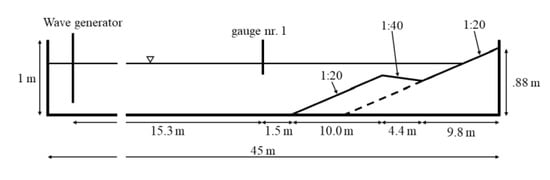
Figure 9.
Schematic of the wave breaking experiment by Battjes and Janssen [57].
The model domain of the present simulation is a rectangle with the size of 18.5 (0 ≤ x ≤ 18.5) by 0.8 m (−0.4 ≤ y ≤ 0.4). The water depth (h) varies according to the following step-wise function:
- if 0 ≤ x ≤ 10, h = 0.616 − 1/20*(x)
- if 10 < x ≤ 14.4, h = 0.116 + 1/40 *(x − 10)
- if 14.4 < x, h = 0.226 − 1/20*(x − 14.4)
Note that the right-most boundary of the baseline run has a water depth of 0.021 m which is arbitrarily small to ensure that the waves break down.
The waves enter the mode domain at x = 0 and propagate in the positive x-direction. At the wave entrance, the wave energy spectrum follows the JONSWAP spectrum distribution with a peak frequency of 0.53 Hz and a significant wave height of 0.2 m. A total of 31 points are used in the frequency space. The frequency points are distributed logarithmically, such that fi = 1.10fi−1, where the subscript i is the frequency point index. This results in the minimum frequency of 0.13 Hz and maximum frequency of 2.21 Hz. Since waves propagate in the x-direction without a current, the directional space discretization is unimportant. Five points are used in the present simulation with the 30o half-angle spread. The default wave breaker parameter of 0.73 is used by other investigators such as Yildirim [46] and so the same is adopted in this study.
The predicted significant wave height is compared with the experimental data in Figure 10. It is seen that SRH-Coast predicts the wave height well. Though not shown here, the SRH-Coast results are also similar to the results of Yildirim [46,55]. The height is slightly under-predicted from x = 0 to 5 m and over-predicted from 5 to 10 m; this is probably due to the omission of the triad wave–wave interactions. The height does not change much in the trough zone (10 to 17 m) as wave breaking is almost non-existent in this zone according to the experiment observation. Towards the right boundary, the wave breaking increases rapidly so that the wave height is approaching zero (100% breaking waves).
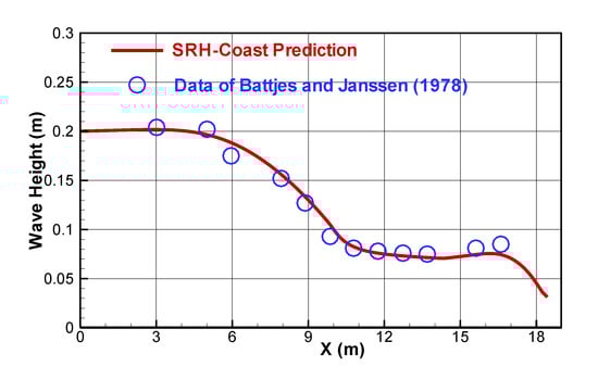
Figure 10.
Comparison of the predicted wave height with the experimental data of Battjes and Janssen [57].
6. Wave Diffraction
Diffraction modeling is verified using the standard case with a semi-infinite breakwater shown in Figure 11. The model domain is rectangular with 15L in the cross-shore (x) direction and 20L in the along-shore (y) direction (L = 100 m, the wavelength of the incoming monochromatic wave). The semi-infinite breakwater is located halfway along the lower boundary pointing upwards and is modeled as a hole in the domain with a thickness of 0.25L.
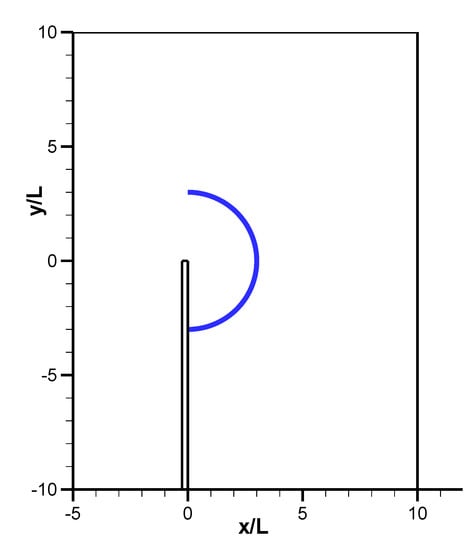
Figure 11.
Layout and model domain for the diffraction modeling behind the semi-infinite breakwater (L is the wave length; blue semi-circle is the arc along which the result is compared).
The case is such designed that the final result may be compared with the analytical solution and other wave models. The travelling monochromatic wave is from left to right in a constant water depth of 5L and with a wave period of 8s. The single frequency is realized by using only one frequency bin. The distribution is used with s = 3000 so that a narrow directional spread is realized (the one-sided half-angle is 3.0°). In the directional space, 31 points are used; in the geographical space, a total of 4800 cells are used. In the simulation, no wave energy smoothing is performed (see discussion in Section 2.4), as our computations showed that smoothing degraded the model accuracy although it promoted stability. We believe that the model accuracy is more important.
The simulated result is shown in Figure 12 in terms of the distribution of the significant wave height; the result without the diffraction treatment is also shown. In Figure 13, the model-predicted significant wave height along the semi-circle of radius 3 L, marked in Figure 11, is compared with the analytical solution of Sommerfeld [72] as well as the result reported by Holthuijsen et al. [58], who used the SWAN model for the simulation. The results show that wave propagation does not show any diffraction behind the semi-infinite plate if the diffraction treatment presented in Section 2.4 is not applied (see Figure 12b and Figure 13). The results without the diffraction treatment demonstrate that the numerical diffusion of the present model is very small: the diffusion thickness is limited to one mesh cell size and there is no spread of the predicted significant wave height passing the breakwater.
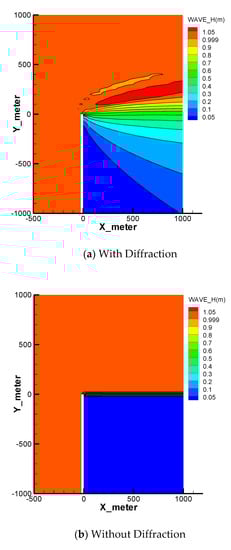
Figure 12.
Contours of the significant wave height predicted by SRH-Coast with and without diffraction activated.
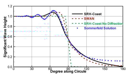
Figure 13.
Comparison of the significant wave height among the SRH-Coast solution, analytical solution of Sommerfeld and SWAN solution along the 3L semi-circle.
When diffraction modeling is activated, the model results are shown in Figure 12a and Figure 13. Note that any wave energy above the level of the without-diffraction run must be due to the diffraction approximation implemented in the model. It is seen that SRH-Coast result is close to the Sommerfeld solution and the match is reasonably good except on either side of the semi-circle. On the left side, small oscillations of the analytical solution are not captured; the overshoot on the exposed side of the shadow line, however, is reproduced well by the model. On the right side in the deep-shadow region (where the significant wave height is less than 0.19), the mismatch is relatively large. This is due to the singularity of the tip of the breakwater that needs other special treatment [58]. SRH-Coast results match better than the SWAN results of Holthuijsen et al. [58] (see Figure 13). It is possible that the smoothing of the wave energy used in the SWAN modeling had contributed to the difference of the model results.
7. Concluding Remarks
In this study, a new wave model is developed that is embedded within the current model SRH-2D for simulating wave propagation and the associated generation and dissipation processes in the near-shore coastal area. Various wave processes are incorporated in the model such as wave shoaling and refraction. In particular, the complex physical processes of wave breaking and wave diffraction are incorporated into the wave model. The theory and numerical solution of diffraction modeling are presented and discussed.
An extensive list of cases is simulated to verify the wave processes of shoaling, refraction, wave breaking and diffraction. These cases are selected to verify that the implementation of the mathematical equations of various physical processes is carried out correctly. The simulated results compare well with the known analytical or measured results and previous model studies for all cases.
The verification study demonstrates that the new wave model is capable of predicting various important wave dynamic processes. The work paves the way to the next phase of the model development: a tightly coupled modeling of the current and wave modules with the one-model approach.
Author Contributions
Conceptualization, Y.G.L., H.K.; methodology, Y.G.L., H.K.; software, Y.G.L., H.K.; validation, Y.G.L., H.K.; writing—original draft preparation, Y.G.L.; writing—review and editing, H.K. All authors have read and agreed to the published version of the manuscript.
Funding
This research was funded by the Water Resources Agency, Taiwan.
Conflicts of Interest
The authors declare no conflict of interest.
References
- Dean, R.G.; Dalrymple, R.A. Coastal Processes with Engineering Applications; Cambridge University Press: Cambridge, UK, 2004. [Google Scholar]
- Davidson-Arnott, R. Introduction to Coastal Processes and Geomorphology; Cambridge University Press: Cambridge, UK, 2009. [Google Scholar]
- Garcia, A.; Rangel-Buitrago, N.; Oakley, J.A.; Williams, A.T. Use of ecosystems in coastal erosion management. Ocean Coast. Manag. 2018, 156, 277–289. [Google Scholar] [CrossRef]
- Álvarez, M.; Carballo, R.; Ramos, V.; Iglesias, G. An integrated approach for the planning of dredging operations in estuaries. Ocean Eng. 2017, 140, 73–83. [Google Scholar] [CrossRef]
- Sengupta, D.; Chen, R.; Meadows, M.E. Building beyond land: An overview of coastal land reclamation in 16 global megacities. Appl. Geogr. 2018, 90, 229–238. [Google Scholar] [CrossRef]
- Lagmay, A.M.F.; Agaton, R.P.; Bahala, M.A.C.; Briones, J.B.L.T.; Cabacaba, K.M.C.; Caro, C.V.C.; Dasallas, L.L.; Gonzalo, L.A.L.; Ladiero, C.N.; Lapidez, J.P.; et al. Devastating storm surges of Typhoon Haiyan. Int. J. Disaster Risk Reduct. 2015, 11, 1–12. [Google Scholar] [CrossRef]
- Brown, J.M.; Phelps, J.J.C.; Barkwith, A.; Hurst, M.D.; Ellis, M.A.; Plater, A.J. The effectiveness of beach mega-nourishment, assessed over three management epochs. J. Environ. Manag. 2016, 184, 400–408. [Google Scholar] [CrossRef]
- Carrasco, A.R.; Ferreira, Ó.; Roelvink, D. Coastal lagoons and rising sea level: A review. Earth Sci. Rev. 2016, 154, 356–368. [Google Scholar] [CrossRef]
- Goldbach, C.; Schlüter, A.; Fujitani, M. Analyzing potential effects of migration on coastal resource conservation in Southeastern Ghana. J. Environ. Manag. 2018, 209, 475–483. [Google Scholar] [CrossRef] [PubMed]
- Sorensen, R.M. Basic Coastal Engineering; Springer: New York, NY, USA, 2006. [Google Scholar]
- Deng, J.; Woodroffe, C.D.; Roger, K.; Harff, J. Morphogenetic modelling of coastal and estuarine evolution. Earth Sci. Rev. 2017, 171, 254–271. [Google Scholar] [CrossRef]
- Kim, H.; Lai, Y.G. Estuary and Coastal Modeling: Literature Review and Model Design; Technical Report No. ENV-2019-034; Technical Service Center, Bureau of Reclamation: Denver, CO, USA, 2019. [Google Scholar]
- Fleming, C.A.; Hunt, J.N. Application of a sediment transport model. In Proceedings of the 15th International Conference on Coastal Engineering, Honolulu, HI, USA, 11–17 July 1976; pp. 1194–1202. [Google Scholar]
- Longuet-Higgins, M.S. Longshore currents generated by obliquely incident sea waves. J. Geophys. 1970, 75, 6779–6789. [Google Scholar]
- Coeffe, Y.; Pechon, P.H. Modelling of sea-bed evolution under waves action. In Proceedings of the 18th International Conference on Coastal Engineering, Cape Town, South Africa, 14–19 November 1982; pp. 1149–1160. [Google Scholar]
- Boer, S.; de Vriend, H.J.; Wind, H.G. A system of mathematical models for the simulation of morphological processes in the coastal area. In Proceedings of the 19th International Conference on Coastal Engineering, Houston, TX, USA, 3–7 September 1984; pp. 1437–1453. [Google Scholar]
- De Vriend, H.J.; Ribberink, J.S. A quasi-3D mathematical model of coastal morphology. In Proceedings of the 21st International Conference on Coastal Engineering, Costa del Sol-Malaga, Spain, 20–25 June 1988; pp. 1689–1703. [Google Scholar]
- Price, D.M.; Chesher, T.J.; Southgate, H.N. PISCES: A Morphodynamic Coastal Area Model; Report, SR 411; HR Wallingford: Wallingford, UK, 1995. [Google Scholar]
- Lou, J.; Ridd, P.V. Modelling of suspended sediment transport in coastal areas under waves and currents. Estuarine. Coast. Shelf Sci. 1997, 45, 1–16. [Google Scholar]
- Deltares. Delft3D-WAVE. In User Manual; Version 3.15.34160; Deltares: Delft, The Netherlands, 2014. [Google Scholar]
- Hervouet, J.M.; Bates, P. The TELEMAC modelling system—Special issue. Hydrol. Process. 2000, 14, 2207–2208. [Google Scholar] [CrossRef]
- Ding, Y.; Wang, S.S.Y. Development and application of a coastal and estuarine morphological process modeling system. J. Coast. Res. 2008, 52, 127–140. [Google Scholar] [CrossRef]
- Klingbeil, K.; Lemarié, F.; Debreu, L.; Burchard, H. The numerics of hydrostatic structured-grid coastal ocean models: State of the art and future perspectives. Ocean Model. 2018, in press. [Google Scholar] [CrossRef]
- Lu, Y.; Li, S.; Zuo, L.; Liu, H.; Roelvink, J.A. Advances in sediment transport under combined action of waves and currents. Int. J. Sediment Res. 2015, 30, 351–360. [Google Scholar] [CrossRef]
- Amoudry, L.O.; Souza, A.J. Deterministic coastal morphological and sediment transport modeling: A review and discussion. Rev. Geophys. 2011, 49, RG2002. [Google Scholar] [CrossRef]
- Booij, N.; Ris, R.C.; Holthuijsen, L.H. A third-generation wave model for coastal regions: 1. Model description and validation. J. Geophys. Res. 1999, 104, 7649–7666. [Google Scholar] [CrossRef]
- SWAN Team. SWAN–Scientific and Technical Documentation; Delft University of Technology: Delft, The Netherlands, 2018; Available online: http://www.swan.tudelft.nl (accessed on 5 February 2020).
- Luo, J.; Li, M.; Sun, Z.; O’Connor, B.A. Numerical modelling of hydrodynamics and sand transport in the tide-dominated coastal-to-estuarine region. Mar. Geol. 2013, 342, 14–27. [Google Scholar] [CrossRef]
- Jia, Y.; Wang, S.S.Y. CCHE2d: Two-Dimensional Hydrodynamics and Sediment Transport Model for Unsteady Open Channel Flows over Loose Bed; Technical Report, No. NCCHE-TR-2001-1; National Center for Computational Hydroscience and Engineering: University, MS, USA, 2001. [Google Scholar]
- Larson, M.; Kraus, N.C. Numerical model of longshore current for bar and trough beaches. J. Waterw. Port Coast Ocean Eng. 1991, 117, 326–347. [Google Scholar] [CrossRef]
- Janssen, P.A.E.M. Progress in ocean wave forecasting. J. Comput. Phys. 2008, 227, 3572–3594. [Google Scholar] [CrossRef]
- Hasselmann, K.; Barnett, T.P.; Bouws, E.; Carlson, H.; Cartwright, D.E.; Enke, K.; Ewing, J.A.; Gienapp, H.; Hasselmann, D.E.; Kruseman, P.; et al. Measurements of wind-wave growth and swell decay during the Joint North Sea Wave Project (JONSWAP). Dtsch. Hydrogr. Z. 1973, 12, A8. [Google Scholar]
- WAMDI Group. The WAM Model—A third generation ocean wave prediction model. J. Phys. Oceanog. 1988, 18, 1775–1810. [Google Scholar] [CrossRef]
- SWAMP Group; Sea Wave Modeling Project. Ocean Wave Modeling; Plenum Pub Corp.: New York, NY, USA, 1985. [Google Scholar]
- Hasselmann, S.; Hasselmann, K.; Allender, J.H.; Barnett, T.P. Computations and parameterizations of the nonlinear energy transfer in a gravity wave spectrum. Part II: Parameterizations of the nonlinear transfer for application in wave models. J. Phys. Oceanogr. 1985, 15, 1378–1391. [Google Scholar] [CrossRef]
- Komen, G.J.; Hasselmann, S.; Hasselmann, K. On the existence of a fully developed wind-sea spectrum. J. Phys. Oceanogr. 1984, 14, 1271–1285. [Google Scholar] [CrossRef]
- Tolman, H.L. A third-generation model for wind waves on slowly varying, unsteady, and inhomogeneous depths and currents. J. Phys. Oceanogr. 1991, 21, 782–797. [Google Scholar] [CrossRef]
- Benoit, M.; Marcos, F.; Becq, F. Development of a Third Generation Shallow Water Wave Model with Unstructured Spatial Meshing, Proc. 25th Int. Conf. Coastal Engineering (Orlando); ASCE: New York, NY, USA, 1996; pp. 465–478. [Google Scholar]
- Sorensen, O.R.; Kofoed-Hansen, H.; Rugbjerg, M.; Sorensen, L.S. A third-generation spectral wave model using an unstructured finite volume technique. In Coastal Engineering Conference; American Society of Civil Engineers: Reston, VA, USA, 2004; Volume 29, p. 894. [Google Scholar]
- Roland, A.; Zanke, U.; Hsu, T.W.; Ou, S.H.; Liau, J.M.; Wang, S.K. Verification of a 3rd generation FEM spectral wave model for shallow and deep water applications. ASME Conf. Proc. 2006, 2006, 487–499. [Google Scholar]
- Hsu, T.W.; Ou, S.H.; Liau, J.M. Hindcasting nearshore wind waves using a FEM code for SWAN. Coast. Eng. 2005, 52, 177–195. [Google Scholar] [CrossRef]
- Qi, J.; Chen, C.; Beardsley, R.C.; Perrie, W.; Cowles, G.W.; Lai, Z. An unstructured-grid finite-volume surface wave model (FVCOM-SWAVE): Implementation, validations and applications. Ocean Model. 2009, 28, 153–166. [Google Scholar] [CrossRef]
- Zijlema, M. Computation of wind-wave spectra in coastal waters with SWAN on unstructured grids. Coast. Eng. 2010, 57, 267–277. [Google Scholar] [CrossRef]
- Rusu, E. Reliability and Applications of the Numerical Wave Predictions in the Black Sea. Front. Mar. Sci. 2016, 3, 95. [Google Scholar] [CrossRef]
- Anton, I.A.; Rusu, L.; Anton, C. Nearshore Wave Dynamics at Mangalia Beach Simulated by Spectral Models. J. Mar. Sci. Eng. 2019, 7, 206. [Google Scholar] [CrossRef]
- Yildirim, B.G.; Karniadakis, G.E. A hybrid spectral/DG method for solving the phase-averaged ocean wave equation: Algorithm and validation. J. Comput. Phys. 2012, 231, 4921–4953. [Google Scholar] [CrossRef]
- Meixner, J.D. Discontinuous Galerkin Methods for Spectral Wave-Circulation Modeling. Ph.D. Thesis, The University of Texas at Austin, Austin, TX, USA, 2013. [Google Scholar]
- Kim, K.O.; Yun, J.-H.; Choi, B.H. Simulation of Typhoon Bolaven using integrally coupled tide-surge-wave models based on locally enhanced fine-mesh unstructured grid system. J. Coast. Res. 2016, 75, 1127–1131. [Google Scholar] [CrossRef]
- Farhadzadeh, A.; Gangai, J. Numerical modeling of coastal storms for ice-free and ice-covered Lake Erie. J. Coast. Res. 2017, 33, 1383–1396. [Google Scholar] [CrossRef]
- Qu, K.; Tang, H.S.; Agrawal, A. Integration of fully 3D fluid dynamics and geophysical fluid dynamics models for multiphysics coastal ocean flows: Simulation of local complex free-surface phenomena. Ocean Model. 2019, 135, 14–30. [Google Scholar] [CrossRef]
- Cavaleri, L.; Barbariol, F.; Benetazzo, A.; Waseda, T. Ocean Wave Physics and Modeling: The Message from the 2019 WISE Meeting. Bull. Am. Meteorol. Soc. 2019, 100, ES297–ES300. [Google Scholar] [CrossRef]
- Lai, Y.G. SRH-2D Version 2: Theory and User’s Manual; Technical Service Center, Bureau of Reclamation: Denver, CO, USA, 2008. [Google Scholar]
- Lai, Y.G. Two-Dimensional Depth-Averaged Flow Modeling with an Unstructured Hybrid Mesh. J. Hydraul. Eng. 2010, 136, 12–23. [Google Scholar] [CrossRef]
- Holthuijsen, L.H. Waves in Oceanic and Coastal Waters; Cambridge University Press: Cambridge, UK, 2007. [Google Scholar]
- Lai, Y.G.; Kim, H. Estuary and Coastal Modeling: Wave Module Development and Verification; Technical Report No. ENV-2020-029; Technical Service Center, Bureau of Reclamation: Denver, CO, USA, 2020. [Google Scholar]
- Lin, L.; Demirbilek, Z.; Mase, H.; Zheng, J.; Yamada, F. CMS-Wave: A nearshore spectral wave processes model for coastal inlets and navigation projects. In Technical Report ERDC/CHL TR-08-13; U.S. Army Engineer Research and Development Center, Coastal and Hydraulics Laboratory: Vicksburg, MS, USA, 2008. [Google Scholar]
- Battjes, J.A.; Janssen, J.P.F.M. Energy loss and set-up due to breaking of random waves. In Proceedings of the 16th International Conference on Coastal Engineering, Hamburg, Germany, 27 August–3 September 1978; pp. 569–587. [Google Scholar]
- Holthuijsen, L.H.; Hermanb, A.; Booija, N. Phase-decoupled refraction–diffraction for spectral wave models. Coast. Eng. 2003, 49, 291–305. [Google Scholar] [CrossRef]
- Hsu, T.W.; Ou, S.H.; Liau, J.M. WWM extended to account for wave diffraction on a current over a rapidly varying topography. In Proceedings of the Third Chinese-German Joint Symposium on Coastal and Ocean Engineering (JOINT2006), Tainan, Taiwan, 25 August 2006. [Google Scholar]
- Mase, H. Multidirectional random wave transformation model based on energy balance equation. Coast. Eng. J. 2001, 43, 317–337. [Google Scholar] [CrossRef]
- Sanchez, A.; Wu, W.; Beck, T.M. A depth-averaged 2-D model of flow and sediment transport in coastal water. Ocean Dyn. 2016, 66, 1475–1495. [Google Scholar] [CrossRef]
- Enet, F.; Nahon, A.; van Vledder, G.; Hurdle, D. Evaluation of diffraction behind a semi-infinite breakwater in the SWAN Wave Model. In Proceedings of the Ninth International Symposium on Ocean Wave Measurement and Analysis—WAVES06, Emmeloord, Alkyon, 8–16 November 2006. [Google Scholar]
- Bertotti, L.; Cavaleri, L. Accuracy of wind and wave evaluation in coastal regions. In Proceedings of the 24th International Conference on Coastal Engineering, Kobe, Japan, 23–28 October 1994. [Google Scholar]
- Mitsuyasu, H.; Tsai, F.; Subara, T.; Mizuno, S.; Ohkusu, M.; Honda, T.; Rikiishi, K. Observation of the Directional Spectrum of Ocean Waves Using a Cloverleaf Buoy. J. Phys. Oceanogr. 1975, 5, 750–760. [Google Scholar] [CrossRef]
- Boris, J.P.; Book, D.L. Flux corrected transport I, SHASTA, a fluid transport algorithm that works. J. Comput. Phys. 1973, 11, 38–69. [Google Scholar] [CrossRef]
- Lai, Y.G. Unstructured grid arbitrarily shaped element method for fluid flow simulation. AIAA J. 2000, 38, 2246–2252. [Google Scholar] [CrossRef]
- Adam, A. Finite Element, Adaptive Spectral Wave Modelling. Ph.D. Thesis, Imperial College London, London, UK, 2016. [Google Scholar]
- Philips, O.M. The Dynamics of the Upper Ocean. In Cambridge Monographs on Mechanics; Cambridge University Press: Cambridge, UK, 1977. [Google Scholar]
- Mei, C.C.; Stiassnie, M.; Yue, D.K.P. Theory and Applications of Ocean Surface Waves: Nonlinear aspects. Advanced series on ocean engineering. World Sci. 2005, 23, 1071. [Google Scholar]
- Longuet-Higgins, M.S.; Stewart, R.W. The changes in amplitude of short gravity waves on steady non-uniform currents. J. Fluid Mech. 1961, 10, 529–549. [Google Scholar] [CrossRef]
- Shemdin, O.H.; Hsiao, S.V.; Carlson, H.E.; Hasselmann, K.; Schulze, K. Mechanisms of wave transformation in finite depth water. J. Geophys. Res. 1980, 85, 5012–5018. [Google Scholar] [CrossRef]
- Sommerfeld, A. Mathematische theorie der diffraktion. Mathematische Annalen. 1896, 47, 317–374. [Google Scholar] [CrossRef]
Publisher’s Note: MDPI stays neutral with regard to jurisdictional claims in published maps and institutional affiliations. |
© 2020 by the authors. Licensee MDPI, Basel, Switzerland. This article is an open access article distributed under the terms and conditions of the Creative Commons Attribution (CC BY) license (http://creativecommons.org/licenses/by/4.0/).