Abstract
Aerodynamic development for road vehicles is usually carried out in a uniform steady-state flow environment, either in the wind tunnel or in Computational Fluid Dynamics (CFD) simulations. However, out on the road, the vehicle experiences unsteady flow with fluctuating angles of incidence , caused by natural wind, roadside obstacles, or traffic. In order to simulate such flow fields, the Forschungsinstitut für Kraftfahrwesen und Fahrzeugmotoren Stuttgart (FKFS) swing® system installed in the quarter scale model wind tunnel can create a variety of time-resolved signals with variable . The static pressure gradient in the empty test section, as well as values of the Society of Automotive Engineers (SAE) body and the DrivAer model, have been measured under these transient conditions. The measurements have been corrected using the Two-Measurement Correction method in order to decouple the influence of the unsteady flow from that of the static pressure gradient. The investigation has determined that the static pressure gradient in the empty test section varies greatly with different excitation signals. Thus, it is imperative to apply a correction for unsteady wind tunnel measurements. The corrected values show that a higher signal amplitude, as in, signals with large , lead to higher drag forces. The influence of the signal frequency on drag values varies depending on the vehicle geometry and needs to be investigated further in the future.
1. Introduction
Wind tunnel testing is employed during automobile development, in order to optimize a car’s aerodynamic properties, as well as during certification, to determine a car’s fuel economy. In both cases, the test engineer operates under the assumption that the measured aerodynamic coefficients, especially aerodynamic drag, are equal to the ones the vehicle experiences on the road. There are two main reasons why this is not the case: One is the finite geometry of the wind tunnel and the other is the transient flow experienced by the on-road vehicle.
The finite geometry of the wind tunnel creates a flow field in the test section that differs from the one a vehicle experiences on the road. Therefore, the measured value in the wind tunnel needs to be corrected to simulate the on-road case more accurately. For the open jet wind tunnel, which is ubiquitous in the auto industry, the current state of the art correction method is the Two-Measurement Correction by Mercker and Cooper [1], with an addendum by Hennig [2]. This correction method has been developed from the Mercker/Wiedemann correction published in 1996 [3] and uses physical models to quantify different interference effects, such as nozzle blockage and horizontal buoyancy [1,3]. Mercker and Cooper have proven the effectiveness of the Two-Measurement Correction through measurements in different wind tunnel configurations. Once the correction has been applied, the previously measured, highly deviating values for a single vehicle have converged to approximately the same value [1].
The transient flow experienced by the on-road vehicle is another phenomenon the typical wind tunnel cannot simulate, because the flow field in a wind tunnel test section is typically uniform, stationary and parallel to the direction of travel. Turbulence and nonzero yaw angles occurring during on-road driving, as described by Cooper, Watkins [4], Lawson [5] and Jessing [6], will potentially yield different values compared to those measured in a wind tunnel. In order to simulate turbulence and fluctuating yaw angles, several automobile full-scale and model scale wind tunnels have added systems to create transient incident flow. Among these are the Pininfarina wind tunnel [7,8] and more recently Durham University’s model scale tunnel [9] as well as Toyota’s new full-scale tunnel [10].
At the University of Stuttgart, the Forschungsinstitut für Kraftfahrwesen und Fahrzeugmotoren Stuttgart (FKFS) swing® system has been developed by Schröck [11] and subsequently installed in both the full-size and model size wind tunnels. Using this system, Stoll has investigated both the side force and yaw moment response [12], as well as the aerodynamic drag of the DrivAer model [13], under the influence of two excitation signals simulating on-road flow. For the drag investigation, the Two-Measurement Correction has been applied.
This paper aims to continue this line of investigations with respect to unsteady drag. To this end, a variety of filtered random noise and sine signals have been used as excitation input for the FKFS swing® system. The measurements in the model scale wind tunnel show the influence different signals have on both the airflow in the empty test section and the value of different test vehicles.
2. Experimental Setup
All experimental investigations described in this paper were carried out in the model scale wind tunnel at the Institute of Automotive Engineering (IFS) of the University of Stuttgart. It has a closed air circuit and open jet test section with a nozzle cross-sectional area of 1.6 m2. The wind tunnel is equipped with a rotating turntable and a state-of-the-art ground simulation system, including 5-belt- and boundary layer manipulation systems. However, all measurements in this study were carried out without any ground simulation. A dynamic underfloor balance is installed in the test section to measure the unsteady aerodynamic forces and moments [14]. All measurements were carried out at a freestream velocity of = 45 m/s. The vehicle measurements were performed without underhood flow (closed grill). In order to perform the corrections, it is necessary to change the static pressure distribution in the test section. To this end, stagnation bodies of different sizes can be placed in the collector.
2.1. Unsteady Incident Flow with the FKFS swing® System
As previously mentioned, the IFS Model Scale Wind Tunnel employs the FKFS swing® system to generate an unsteady incident yaw angle. The system consists of six identical, vertical wings, aligned at the nozzle exit (Figure 1). The system can operate at a maximum freestream velocity of 50 m/s while achieving a maximum yaw angle and frequency of 10° and 12 Hz, respectively [11,12]. In order to describe the resulting flow conditions, a fast-response cobra probe in the center of the empty test section at z = 250 mm was used to measure the incident yaw angle for each applied excitation signal.
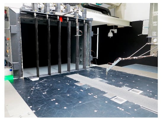
Figure 1.
Forschungsinstitut für Kraftfahrwesen und Fahrzeugmotoren Stuttgart (FKFS) swing® in the Institute of Automotive Engineering Stuttgart (IFS) model scale wind tunnel, with cobra probes measuring flow angles.
For this study, two types of unsteady signals were applied: Filtered random noise signals and sine signals. The noise signals are created using a random number distribution to determine the flap angle over time, cutting off angles above 10° to ensure operational safety, then applying a first-order Butterworth low-pass filter with the cutoff frequency . The resulting yaw angle probabilities show a roughly normal (Gaussian) distribution (Figure 2. Therefore, the noise signals are sufficiently characterized using their cutoff frequency and their standard deviation . The noise signals’ yaw angle distributions are similar to those observed during Jessing’s on-road measurements [6]. Thus, they offer a good representation of the on-road incident flow environment.
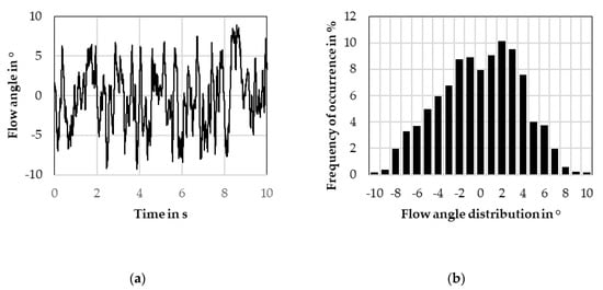
Figure 2.
(a) Flow angle time history for a filtered random noise signal ( = 7.5 Hz, = 3.8°); (b) Flow angle probability distribution for the same signal.
The other type of signal used, the sine signal, can be characterized using its frequency and its amplitude . In addition, it is possible to calculate the standard deviation for the sine signal as well, using the formula:
Contrary to the noise signal, sine signals cannot realistically represent on-road conditions, because their yaw angle distributions are entirely different (Figure 3). However, unlike the noise signal, the sine signal only has one frequency in its spectrum, potentially making it easier to discover and understand correlations between the signal and the wind tunnel or vehicle reactions.
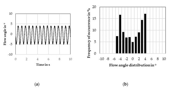
Figure 3.
(a) Flow angle time history for a sine signal ( = 1.5 Hz, = 4.4°); (b) Flow angle probability distribution for the same signal.
In this paper, 16 different noise signals and 20 different sine signals were used for the investigations. Appendix A contains the signals’ characteristic values.
2.2. Test Vehicles
While the focus of the study has been responses to different incident flow signals, four different test vehicles were used in order to investigate the influence of the unsteady flow on different shapes. The quarter scale Society of Automotive Engineers (SAE) reference body was measured in both its squareback and notchback configuration (Figure 4), as has the quarter scale DrivAer model (Figure 5). The different models allow both comparisons between different rear end shapes, as well as between the abstract shape of the SAE body and the higher level of detail of the DrivAer.
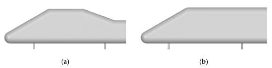
Figure 4.
(a) Society of Automotive Engineers (SAE) reference body, notchback; (b) SAE reference body, squareback.
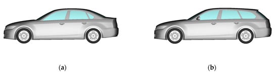
Figure 5.
(a) DrivAer model, notchback; (b) DrivAer model, squareback.
3. Evaluation Methods for Pressure and Drag Measurements
This section will detail the utilized execution and post-processing of the pressure and measurements. It will introduce a quantifiable value for the static pressure gradient in the empty wind tunnel test section, describe the measures taken for the correction, as well as reiterate the definition of the quasi-steady aerodynamic drag.
3.1. The Static Pressure Gradient
Most commonly, the nonzero static pressure gradient in an empty wind tunnel test section is caused by nozzle or collector interference [3], or boundary layer control mechanisms [15]. The nozzle gradient stems from insufficient adaptation of the static pressure in the nozzle exit to the ambient pressure, while the jet’s shear layer stagnating at the collector entry create the gradient there [3]. Both these interference effects are dependent on the wind tunnel geometry. Boundary layer control systems, such as suction mechanisms, can change the static pressure immensely at the vehicle front [15]. However, this is not a consideration for this study since the experiments were carried out without ground simulation.
This static pressure gradient in the test section induces an error in measurements because outside the wind tunnel, in an infinite freestream, the pressure distribution is constant along the direction of travel. Therefore, the pressure gradient plays an important role in wind tunnel correction methods [1,3]. Since the gradient is a function of wind tunnel geometry, it stands to reason that changes in said geometry, like the movement of the FKFS swing® wings, will also change the gradient.
To measure the static pressure distribution in x-direction, a Prandtl probe was placed in the empty test section at y = 0 and z = 150 mm. For every signal, the probe was moved along the x-axis from x = 900 mm (close to the nozzle) to x = −900 mm (close to the collector) in 100 mm steps. At each measurement point, the pressure measurement was averaged over 30 s. The measured static pressure function over the x-position was then smoothed by using a fourth-order polynomial for both the front and back of the curve. Figure 6 shows an example of this process:
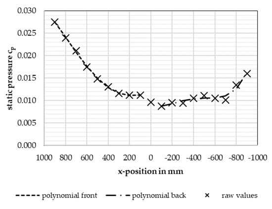
Figure 6.
Static pressure distribution in the empty test section (sine signal; = 1.5 Hz, = 4.4°).
The Two-Measurement method uses the pressure difference between the position at the vehicle’s front bumper and a sensitivity point at the rear of the vehicle to correct the measured [1]. In order to quantify the pressure gradient with respect to its influence on measured , only pressure deltas need to be observed. For this study, the pressure gradient was thus defined as:
Here, is the position of the SAE body’s front bumper when placed in the test section, whereas is the position a quarter-vehicle length behind the rear bumper of the SAE body. This value was chosen because the aforementioned sensitivity point is located at roughly that position for most measurements with the SAE squareback model. It would be possible, and equally valid, to choose different and values derived from other test vehicles. However, the choice of and hardly influences the comparison between gradients measured during different swing® excitation signals.
For the pressure distribution shown in Figure 6, the gradient value is = −3.8·103, or −3.8 counts. The negative value shows a decreasing static pressure towards the collector, meaning that the pressure distribution will artificially add to the measured values. For a positive gradient value, the opposite would be true.
3.2. Unsteady and Quasi-Steady Aerodynamic Drag
As mentioned in Section 2, the model scale wind tunnel uses a dynamic underfloor balance to measure unsteady aerodynamic forces and moments. The results are averaged over 30 s to obtain one set of mean aerodynamic coefficients for each signal input and vehicle.
Additionally, a quasi-steady approach was used to compare the unsteady to one derived from stationary incident flow under yaw. For this, the definition of the quasi-steady aerodynamic drag by Stoll [13] was used. It is an average of values determined during a steady-state yaw sweep, weighted using the flow angle probabilities of the respective incident flow signals. Detailed equations are found in Stoll’s paper [13].
3.3. Correction
The Two-Measurement Correction [1] with Hennig’s addendum [2] is the state-of-the-art correction method. Its validity has been shown for steady incident flow conditions [1], but not for the transient ones evaluated in this study. Therefore, to judge the validity of the correction, all measurements were performed not in two, but in three wind tunnel configurations: The standard configuration, one with small stagnation bodies in the collector, and one with large ones. Since two measurements are required for the correction, three different corrected values can be obtained from one data point: “standard tunnel” corrected with “small stagnation bodies”, “standard tunnel” corrected with “large stagnation bodies”, and “small stagnation bodies” corrected with “large stagnation bodies”. Ideally, these three corrected values should be identical. Thus, the difference between the corrected values for each data point will be a good indicator for the quality of the correction.
For the drag evaluations, the mean value between the three corrected values for each data point was used. For the quasi-steady approach mentioned above, the steady state yaw sweep was corrected first, and the weighted averages determined after. Details on the Two-Measurement Correction method can be found in the quoted sources.
4. Experimental Results
This section will show and discuss the results of the investigation. The pressure gradient in the empty test section, under different transient flow conditions, will be shown. Thereafter, the quality of the corrections will be discussed. A comparison between corrected and uncorrected values will be made, and then the influence of the different flow signals on the different vehicles’ values analyzed.
4.1. Empty Test Section Results
Figure 7 shows all measured data points for the pressure gradient (calculated using Equation (2)) in the standard model wind tunnel configuration. It is important to reiterate that the shown values for and are the flow characteristics measured by the cobra probe, as opposed to the angles entered into the FKFS swing® system. The frequencies, on the other hand, have been shown to remain constant between the input and the flow measurement (this can be observed well in Figure 3), and thus the input frequencies are shown in the following diagrams.
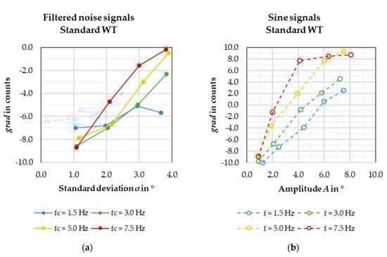
Figure 7.
(a) Pressure gradients in the empty test section for the filtered noise signals, in the standard wind tunnel configuration; (b) Pressure gradients for the sine signals under the same conditions.
Looking at the individual curves, it is evident that the pressure gradient increases with increasing standard deviation or amplitude of the signal, that is, with increasing average incident yaw. Two exceptions to this observation are evident in the diagrams.
One is the red curve in the right figure, showing sine signals at = 7.5 Hz. From an amplitude of roughly 3° upward, the measured gradient barely increases. Since the yellow curve ( = 5 Hz) also slightly stalls at high amplitudes, it is possible that the positive gradient caused by oblique flow possesses an upper limit. The increased static pressure near the collector is likely caused by either a lower local flow velocity due to the jet from the nozzle swinging from side to side, or the impact and stagnation of the oblique jet at the collector mouth, or both. It is reasonable to assume that neither of these phenomena can be amplified endlessly by an increasing flow angle. Future Computational Fluid Dynamics (CFD) investigations may be able to shed more light on these assumptions.
The other exception is the low sensitivity to changes in for the noise signals with a cutoff frequency of = 1.5 Hz. The low frequency is not a sufficient explanation, because the sine signals at = 1.5 Hz show an increasing gradient with increasing amplitude. Again, CFD investigations will be necessary to formulate an explanation.
Next, comparing the different curves, it is visible that the signal frequency influences the static pressure gradient. For the sine signals, it is clear that increasing frequency leads to increasing gradients. The exceptions are found at either very low flow angles or high flow angles for high frequencies. The lack of correlation at low amplitudes can be explained with the generally low influence a small flow angle has on the gradient. At high frequency and amplitude, it can be explained the same way as before—most likely a cap on the gradient number has been reached.
For the noise signals, the positive correlation between the cutoff frequency and the pressure gradient also exists but is much weaker compared to the sine signals’. At low frequencies especially, the gradients of signals with the same flow angle but different tend to be similar. Since a signal with the cutoff frequency also contains all frequencies below , the signals are more similar to each other than the sine signals. This may explain the weaker correlation compared to the sine signals.
As previously mentioned, the sine signal’s amplitude can be converted to a standard deviation σ using Equation (1). This allows the depiction of the gradient results in a single diagram (Figure 8):
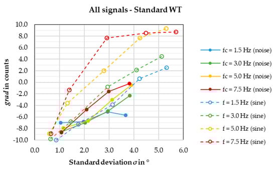
Figure 8.
Pressure gradients in the empty test section for all measured signals, in the standard wind tunnel configuration, in one diagram.
Generally, sine signals seem to create a higher gradient than noise signals. Furthermore, it can be observed when comparing a noise signal to a sine signal, where the noise signal’s is equal to the sine signal’s , that the gulf in gradient becomes higher at higher frequencies. Likely, this is a result of low frequency bands still present in all the noise signals. The frequency spectrum difference naturally becomes more pronounced at high frequencies, since the noise signal still contains all frequencies lower than its .
4.2. Correction Results
As mentioned in Section 3.3, each data point was measured three times with different wind tunnel configurations, then corrected three separate times. Ideally, the three resulting corrected values should be identical. To reiterate the validity of the correction method for steady-state measurements, the different corrected values of the DrivAer notchback’s steady-state yaw sweep is presented in Figure 9. The yaw sweep was measured with mounted, but stationary, flaps, with the yaw angle created by rotating the turntable.
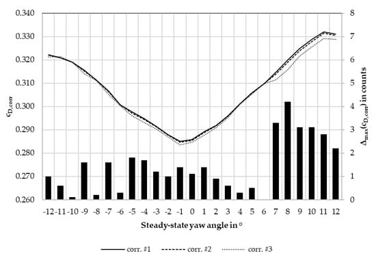
Figure 9.
Corrected values for the DrivAer notchback steady-state yaw sweep and maximum delta between the three corrected values.
The figure also shows the maximum difference between the three corrected values for each data point. The maximum delta is always smaller than 2.0 counts, except for yaw angles above 6°. Such large yaw angles are rarely found during on-road driving [6]. Therefore, the correction does indeed work well for a steady incident flow. For further use within this study, the three corrected steady-state values have been averaged for every data point in order to present one discrete value for each measurement case.
To evaluate the validity of the correction for the unsteady case, the same maximum delta calculation was made and is shown in Figure 10 and Figure 11, again for the DrivAer notchback.
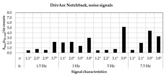
Figure 10.
Maximum delta between the three corrected values for the DrivAer notchback, measured with noise signals.
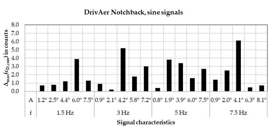
Figure 11.
Maximum delta between the three corrected values for the DrivAer notchback, measured with sine signals.
With the applied transient incident flow shown here, about half of the data points show a maximum delta of less than 2.0 counts, while a quarter show a maximum delta of more than 3.0 counts. As visible in Figure 10 and Figure 11, the signals that cause high delta values between the different corrected values do not follow any pattern, which is also the case for the other vehicles measured. Therefore, the three different corrected values have been averaged for the evaluations in this paper in order to improve the consistency of the correction method.
Figure 12 below compares uncorrected drag values to their corrected counterparts, which have been obtained using the averaging method described previously. It shows why a correction is indispensable for an unsteady flow evaluation.
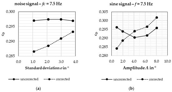
Figure 12.
Drag development of the DrivAer notchback over yaw magnitude, uncorrected vs. corrected, for (a) noise signals and (b) sine signals.
Logically, an increase in aerodynamic drag would be expected with increasing yaw magnitudes of the incident flow signal. After all, steady-state yaw sweeps usually show increased drag for increased yaw (see Figure 9). However, in Figure 12, the uncorrected stays roughly level with increasing and . After the correction was applied, the expected behavior of increasing with increasing and can be observed. The correction takes into account many factors, such as nozzle blockage or jet expansion [1], but mainly it eliminates the influence the different pressure gradients from different signals have on the measured . Therefore, the corrected value reflects the influence of the transient incident flow on the vehicle more accurately. Neglecting the application of a correction means measuring not only the influence of the signal on the vehicle, but also its interaction with the wind tunnel. Since the wind tunnel does not exist in the on-road use case, this is to be avoided.
4.3. Vehicle Drag Results
The drag results for the DrivAer and SAE body notchback and squareback models are discussed. Figure 13 below shows the corrected drag numbers for the DrivAer notchback model.
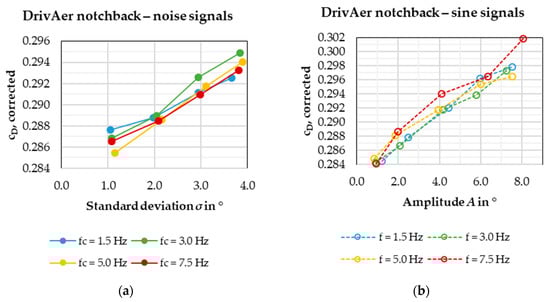
Figure 13.
(a) Corrected for the DrivAer notchback model, measured with the noise signals. (b) Corrected measured with the sine signals.
As expected, the aerodynamic drag increases with increasing flow angles ( or ). Interestingly, the measured drag does not seem to correlate with the signal’s frequency content at all. For both the noise and sine signals, the drag values stay in a corridor of roughly 3 counts for the same signal standard deviation or amplitude.
Figure 14 converts the sine signals’ amplitudes to standard deviation values via Equation (1), as Figure 8 has done in Section 4.1. It is evident that even the type of signal—noise or sine—does not influence the value as long as the signal’s standard deviation remains the same. All curves are in the same corridor of roughly 3 counts for the same .

Figure 14.
Corrected for the DrivAer notchback model, in one diagram.
Next, the quasi-steady values are added to the analysis. For every measured data point, a corresponding quasi-steady drag has been determined (see Section 3.2). Those are added to Figure 14 above, which results in Figure 15 below.
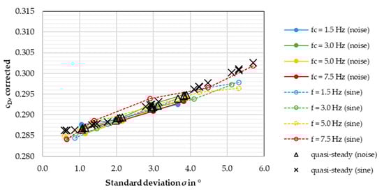
Figure 15.
Corrected for the DrivAer notchback model, in one diagram, with quasi-steady drag.
The quasi-steady drag values, which have been measured in a steady incident flow environment, place squarely within the drag corridor of roughly 3 counts established before. This supports the assumption that the frequency, the whole unsteady behavior even, does not influence the aerodynamic drag. Should this prove true, measurements with transient yaw would become superfluous, since the same results could theoretically be obtained by steady-state measurements.
Figure 16, Figure 17 and Figure 18 below show the test results for the DrivAer squareback and the two SAE reference bodies.
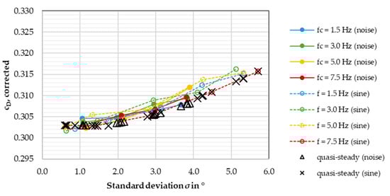
Figure 16.
Corrected for the DrivAer squareback model, in one diagram, with quasi-steady drag.
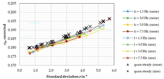
Figure 17.
Corrected for the SAE notchback model, in one diagram, with quasi-steady drag.
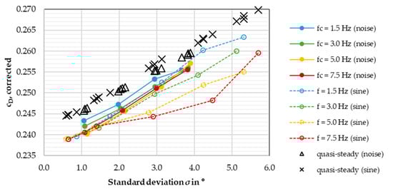
Figure 18.
Corrected for the SAE squareback model, in one diagram, with quasi-steady drag.
For both the DrivAer squareback and the SAE notchback, the previously made assumption seems to remain valid. In both Figure 16 and Figure 17, the drag values stay in a corridor of roughly 4 counts for the same standard deviation, and there is no discernible correlation between and signal frequency. The quasi-steady drag does not match the aforementioned drag corridor but is still right on the edge and follows the general development of the different signals’ graphs. Again, the quasi-steady drag values obtained for the DrivAer squareback and SAE notchback do not conform to the unsteady drag as well as the ones from the DrivAer notchback.
The biggest deviation, however, results for the SAE squareback. As Figure 18 shows, the values measured for the sine signals differ significantly for the same standard deviation, at = 3° and above. There seems to be a clear correlation between frequency and drag for the sine signals—the bigger the frequency, the smaller the drag. Furthermore, the quasi-steady values are always 2–3 counts higher than all unsteady drag values. These results prove that the signal frequency does affect the aerodynamic drag, not for all, but for some vehicles. Still, were the sine signal datasets to be removed, the remaining values measured with the noise signals would still fall in a narrow corridor of roughly 4 drag counts for the same . Despite the sine signals acting differently here compared to the other vehicles, the cutoff frequency of the noise signal still has no bearing on the vehicle’s aerodynamic drag.
To summarize, the test results show that aerodynamic drag increases with increasing signal yaw angles for all test vehicles. The effect of the signal frequency, on the other hand, is somewhat unclear. When observing the data for the different test vehicles, it seems that both the rear end shape and the level of detail of the model influence the level of frequency correlation. Both the DrivAer and SAE squareback models show a higher degree of correlation between frequency and than the respective notchback counterparts do. Similarly, for both the notchback and squareback rear end shapes, the degree of correlation is larger for the more abstract SAE body than for the more realistic DrivAer model. The same observation can be made regarding the quasi-steady drag. It represents the unsteady measurements better for the more realistic vehicle model (DrivAer) and for the notchback rear end shape.
Since aerodynamic drag for an automobile is mainly influenced by the rear of the car, it is reasonable to believe that the unsteady incident flow influences drag mainly by changing the wake and the separation behavior. The aforementioned difference between notchback and squareback models could be attributed to their differences in separation area and wake size, despite having the same frontal area. Furthermore, the lack of detail presumably also contributes to a different wake shape for the SAE body, especially due to the lack of wheels. In order to further investigate this line of assumptions, it would be prudent to repeat the measurements in this study on vehicles with different wake sizes, such as the AeroSUV model [16]. Additionally, the influence of the model’s level of detail can be ascertained using the SAE Type K model [17]. Furthermore, the influence of ground simulation must be considered in further investigations.
Finally, research into the effects of periodic jets on bluff body drag suggests that unsteady excitation around the wake area may noticeably influence the body’s base pressure [18]. This phenomenon is possibly in effect in the investigated cases where the signal frequency strongly influences measured drag. However, the aforementioned effects are more pronounced at higher frequencies, with a Strouhal number of 0.8 or larger [18]. This would translate to a frequency of roughly 30 Hz in the context of this paper, which is impossible to achieve with FKFS swing®.
5. Conclusions
The aim of this paper was to quantify the influence of an unsteady incident flow signal on both the conditions in the wind tunnel and on the measured aerodynamic drag. To this end, measurements were undertaken in the IFS Model Scale Wind Tunnel with the FKFS swing® system enabled. A variety of transient incident flow signals were created. The signals were divided into filtered noise signals, which more closely represent on-road flow, and sine signals, which are simpler to describe with only one frequency.
The static pressure gradient, measured in the empty wind tunnel test section, shows clear differences between different signals. Generally, the gradient grows larger (higher pressure near the collector) for higher signal amplitudes and higher signal frequencies. Consequently, the differences in gradients means that corrections are necessary when dealing with unsteady measurements. This was shown with the vehicle drag measurements. Not only does the correction generally provide different values compared to the uncorrected measurement, but the corrected drag graphs also show different overall behavior.
The Two-Measurement Correction applied in this study loses some robustness when dealing with unsteadiness, as opposed to steady measurements. However, it was nonetheless shown that it is vital to apply a correction, because otherwise the measurements will not show the real transient effects at all. Three different corrections were made for each data point, which ideally should result in the same corrected . For steady measurements, the delta between the three corrected values is much lower compared to the unsteady measurements. Still, the margin of error is small enough that the correction is applicable after averaging the three corrected values for each data point. Nevertheless, the correction method should be investigated more closely with respect to unsteady measurements.
The corrected measurements show a positive correlation between signal amplitude and aerodynamic drag for all signals and all test vehicles. However, the correlation between signal frequency and is more ambiguous. For the DrivAer notchback, for example, there is no correlation between frequency and drag, while the SAE squareback’s varies for different frequencies at the same amplitude. The DrivAer squareback’s and SAE notchback’s behaviors place in between the aforementioned extremes. A possible explanation for this observation is that the size and shape of the separation area affects the influence different signal frequencies have on the vehicle’s wake behavior. The level of detail, which is quite different between the DrivAer and the SAE model, most likely also contributes to the observed differences.
The quasi-steady aerodynamic drag was calculated for all unsteady measurements. Its ability to accurately represent the unsteady depends on the vehicle in question. For some vehicle configurations, the quasi-steady drag is a close approximation of the unsteady drag, while for others it differs from the unsteady drag by a significant amount. This underlines the importance of unsteady drag measurements when attempting to simulate on-road conditions.
Author Contributions
X.F. established the paper’s concept, prepared, performed and evaluated the experiments, and drafted this paper. C.J. had input in the conceptual stage, contributed to the experiments and proofread the paper. T.K. is the immediate supervisor, also had input in the conceptual stage and proofread the paper. J.W. and A.W. are the doctoral advisers of X.F. and gave valuable input during the process. All authors have read and agreed to the published version of the manuscript.
Funding
This research received no external funding.
Conflicts of Interest
The authors declare no conflict of interest.
Abbreviations
| CFD | Computational Fluid Dynamics |
| FKFS | Forschungsinstitut für Kraftfahrwesen und Fahrzeugmotoren Stuttgart |
| IFS | Institut für Fahrzeugtechnik, University of Stuttgart |
| SAE | Society of Automotive Engineers |
| swing® | side wind generator |
| Signal amplitude (for sine signals) | |
| Drag coefficient | |
| Pressure coefficient | |
| Signal frequency (for sine signals) | |
| Signal cutoff frequency (for low-pass filtered noise signals) | |
| Pressure gradient in the empty wind tunnel test section | |
| Incident flow yaw angle | |
| Signal standard deviation (for both noise and sine signals) |
Appendix A Transient Signals Used

Table A1.
Filtered noise signals.
Table A1.
Filtered noise signals.
| Cutoff Frequency in Hz | Flap angle Standard Deviation in ° | Measured Flow Angle Standard Deviation in ° |
|---|---|---|
| 1.5 | 0.75 | 1.06 |
| 1.5 | 1.50 | 1.97 |
| 1.5 | 2.25 | 2.95 |
| 1.5 | 3.00 | 3.84 |
| 3.0 | 0.75 | 1.08 |
| 3.0 | 1.50 | 2.04 |
| 3.0 | 2.25 | 2.95 |
| 3.0 | 3.00 | 3.84 |
| 5.0 | 0.75 | 1.15 |
| 5.0 | 1.50 | 2.16 |
| 5.0 | 2.25 | 3.12 |
| 5.0 | 3.00 | 3.90 |
| 7.5 | 0.75 | 1.08 |
| 7.5 | 1.50 | 2.09 |
| 7.5 | 2.25 | 2.99 |
| 7.5 | 3.00 | 3.82 |
Table A2.
Sine signals.
Table A2.
Sine signals.
| Cutoff Frequency in Hz | Flap Angle Amplitude in ° | Measured Flow Angle Amplitude in ° |
|---|---|---|
| 1.5 | 1.20 | 1.23 |
| 1.5 | 2.50 | 2.48 |
| 1.5 | 5.00 | 4.44 |
| 1.5 | 7.50 | 5.98 |
| 1.5 | 10.00 | 7.53 |
| 3.0 | 1.20 | 0.90 |
| 3.0 | 2.50 | 2.07 |
| 3.0 | 5.00 | 4.17 |
| 3.0 | 7.50 | 5.80 |
| 3.0 | 10.00 | 7.25 |
| 5.0 | 1.20 | 0.84 |
| 5.0 | 2.50 | 1.88 |
| 5.0 | 5.00 | 3.94 |
| 5.0 | 7.50 | 6.01 |
| 5.0 | 10.00 | 7.52 |
| 7.5 | 1.20 | 0.92 |
| 7.5 | 2.50 | 1.98 |
| 7.5 | 5.00 | 4.11 |
| 7.5 | 7.50 | 6.34 |
| 7.5 | 10.00 | 8.07 |
References
- Mercker, E.; Cooper, K. A Two-Measurement Correction for the Effects of a Pressure Gradient on Automotive, Open-Jet, Wind Tunnel Measurements. SAE Tech. Pap. 2006. [Google Scholar] [CrossRef]
- Hennig, A. Eine Erweiterte Methode zur Korrektur von Interferenzeffekten in Freistrahlwindkanälen für Automobile. Ph.D. Thesis, University of Stuttgart, Stuttgart, Germany, 2016. [Google Scholar]
- Mercker, E.; Wiedemann, J. On the Correction of Interference Effects in Open-Jet Wind Tunnels. SAE Tech. Pap. 1996. [Google Scholar] [CrossRef]
- Cooper, K.; Watkins, S. The Unsteady Wind Environment of Road Vehicles, Part One: A Review of the On-Road Turbulent Wind Environment. SAE Tech. Pap. 2007. [Google Scholar] [CrossRef]
- Lawson, A.; Sims-Williams, D.; Dominy, R. Effects of On-Road Turbulence on Vehicle Surface Pressures in the A-Pillar Region. SAE Int. J. Passeng. Cars Mech. Syst. 2008, 1, 333–340. [Google Scholar] [CrossRef]
- Jessing, C.; Wittmeier, F.; Wiedemann, J.; Wilhelmi, H.; Dillmann, A. Characterization of the Transient Airflow around a Vehicle on Public Highways. In Proceedings of the 12th FKFS Conference, Progress in Vehicle Aerodynamics and Thermal Management, Stuttgart, Germany, 1–2 October 2019. [Google Scholar]
- Cogotti, A. Generation of a Controlled Level of Turbulence in the Pininfarina Wind Tunnel for the Measurement of Unsteady Aerodynamics and Aeroacoustics. SAE Tech. Pap. 2003. [Google Scholar] [CrossRef]
- Cogotti, A. Update on the Pininfarina “Turbulence Generation System” and its effects on the Car Aerodynamics and Aeroacoustics. SAE Tech. Pap. 2004. [Google Scholar] [CrossRef]
- Mankowski, O.; Sims-Williams, D.; Dominy, R. A Wind Tunnel Simulation Facility for On-Road Transients. SAE Int. J. Passeng. Cars Mech. Syst. 2014, 7, 1087–1095. [Google Scholar] [CrossRef]
- Yamashita, T.; Makihara, T.; Maeda, K.; Tadakuma, K. Unsteady Aerodynamic Response of a Vehicle by Natural Wind Generator of a Full-Scale Wind Tunnel. SAE Int. J. Passeng. Cars Mech. Syst. 2017, 10, 358–368. [Google Scholar] [CrossRef]
- Schröck, D.; Widdecke, N.; Wiedemann, J. Aerodynamic Response of a Vehicle Model to Turbulent Wind. In Proceedings of the 7th FKFS Conference, Progress in Vehicle Aerodynamics and Thermal Management, Stuttgart, Germany, 6–7 October 2009. [Google Scholar]
- Stoll, D.; Kuthada, T.; Wiedemann, J. Unsteady Aerodynamic Vehicle Properties of the DrivAer Model in the IVK Model Scale Wind Tunnel. In Proceedings of the 10th FKFS Conference, Progress in Vehicle Aerodynamics and Thermal Management, Stuttgart, Germany, 29–30 September 2015. [Google Scholar]
- Stoll, D.; Kuthada, T.; Wiedemann, J. Experimental and numerical investigation of aerodynamic drag in turbulent flow conditions. In Proceedings of the iMechE International Conference on Vehicle Aerodynamics, Coventry, UK, 21–22 September 2016. [Google Scholar]
- Wittmeier, F. The Recent Upgrade of the Model Scale Wind Tunnel of University of Stuttgart. SAE Int. J. Passeng. Cars Mech. Syst. 2017, 10, 203–213. [Google Scholar] [CrossRef]
- Wiedemann, J.; Fischer, O.; Jiabin, P. Further Investigations on Gradient Effects. SAE Tech. Pap. 2004. [Google Scholar] [CrossRef]
- Zhang, C.; Tanneberger, M.; Kuthada, T.; Wittmeier, F.; Wiedemann, J.; Nies, J. Introduction of the AeroSUV-A New Generic SUV Model for Aerodynamic Research. SAE Tech. Pap. 2019. [Google Scholar] [CrossRef]
- Kuthada, T.; Pfannkuchen, E.; Wiedemann, J. Evaluation of Cooling Air Drag on a Reference Body. In Proceedings of the 5th MIRA International Vehicle Aerodynamics Conference, Warwick, UK, 13–14 October 2004. [Google Scholar]
- Barros, D.; Borée, J.; Noack, B.; Spohn, A.; Ruiz, T. Bluff body drag manipulation using pulsed jets and Coanda effect. J. Fluid Mech. 2016, 805, 422–459. [Google Scholar] [CrossRef]
© 2020 by the authors. Licensee MDPI, Basel, Switzerland. This article is an open access article distributed under the terms and conditions of the Creative Commons Attribution (CC BY) license (http://creativecommons.org/licenses/by/4.0/).