Article

Direct Numerical Simulation of Water Droplets in Turbulent Flow

Institute of Aerospace Thermodynamics, University of Stuttgart, Pfaffenwaldring 31, 70569 Stuttgart, Germany
*
Author to whom correspondence should be addressed.
Fluids 2020, 5(3), 158; https://doi.org/10.3390/fluids5030158
Submission received: 11 August 2020 / Revised: 7 September 2020 / Accepted: 8 September 2020 / Published: 11 September 2020
(This article belongs to the Special Issue Modelling of Reactive and Non-reactive Multiphase Flows)

Abstract

:
Details on the fall speeds of raindrops are essential in both applications and natural events, such as rain-rate retrieval and soil erosion. Here, we examine the influence of turbulence on the terminal velocity of two water drops of different sizes. For the first time, computations of droplets in turbulent surroundings are conducted with a direct numerical simulation code based on a volume of fluid method. Both the drop surface deformation and internal circulation are captured. The turbulence intensity at the inflow area, as well as the turbulence length scale are varied. In turbulent flow, we find a decline in the terminal velocities for both drops. Based on the study of the wake flow characteristics and drop surface deformation, the decrease in the terminal velocity is found to be directly linked to a shortening of the wake recirculation region resulting from an earlier and more drastic increase in the turbulence kinetic energy in the shear layer. The turbulent surroundings trigger substantial rises in the drop axis ratio amplitude and a slight increase in the drop oscillation frequency, but barely influence the time-averaged drop axis length.

1. Introduction

Details on the fall speeds of raindrops are essential in numerous applications. These include using areal detectors and Doppler radar to estimate drop size distributions [1,2], employing radars to retrieve rainfall rates [3,4,5], modelling of coalescence and collisional breakup processes [6], soil erosion due to the impact of natural rainfall [7,8,9] and telecommunications [10]. In these applications and many others, raindrops of various sizes have been assumed to fall at their terminal velocities v t . The measurements by Gunn and Kinzer of v t of water droplets are regarded as the standard and are still generally used today [11].
However, several recent studies employing a variety of measuring techniques provide proof of the substantial fall speed discrepancies of raindrops under natural rains conditions and challenged the presumption of raindrops falling at their terminal speed. Löfler-Mang and Joss [12] discovered a substantial scattering of raindrop speeds around the terminal velocity v t curve. They associated the scattering with the turbulent air close to the ground and instrumental limitations. Testik et al. [13] found a reduction of around 10% in the fall speed of 1.9 mm raindrops from v t throughout calm wind conditions. They proposed that the increased drag force on the raindrops was triggered by large amplitude oscillations. Using 2D cloud and precipitation probes, Montero-Martinez et al. [14] identified the presence of super-terminal raindrops with sizes less than 0.7 mm during strong rainfall events. An explanation for the presence of super-terminal drops is that large raindrops have broken up into smaller ones and retain the speed of the original larger drop. The existence of super-terminal raindrops was also detected and confirmed by the following work of Larsen et al. [15] and Montero-Martinez and Garcia-Garcia [16]. Niu et al. [17] discovered that the fall velocities of raindrops covered a wide range for all sizes of raindrops in both stratiform and convective rains. Small raindrops (<1.4 mm) exhibit extensive positive mean deviations from their terminal velocities and larger drops with weaker negative deviations from v t . They associated the results with the influence of lower air density and a typical result of combined effects (e.g., turbulence/organised air motions, coalescence/breakup, instrumental errors). Using a C-band polarimetric radar and 2D Video Disdrometer (2DVD), Thurai et al. [18] identified a robust negative skewness and a wide broadening of the fall velocity distribution for 3 mm raindrops in a rain event dominated by an embedded convective line. They suggested that asymmetric horizontal-mode oscillations may result in an increase of the drag and a decrease of drop fall speeds. Montero-Martinez and Garcia-Garcia [16] detected sub-terminal raindrops smaller than 2 mm in size. During windy periods, there exists a larger portion of sub-terminal drops than in calm wind periods. Drop oscillations, the turbulence effect and transverse drift enhancement and deviations in the vertical trajectory were given as potential influential factors for the presence of sub-terminal raindrops. Subsequently, Bringi et al. [19] discovered that during heavy rainfall with strong wind gusts and high-intensity turbulence, the fall velocity distributions for drops of 1.3 mm, 2.0 mm and 3.0 mm were significantly broadened with negative skewness. In the case of 1.3 mm and 2.0 mm drops, the decrease in the mean fall speeds are stronger, with a maximum decrease around 25–30% below v t . With higher turbulence strength, the decrease in mean fall speeds was found to be more significant.
In the present study, we examine the influence of turbulence on falling water drops through Direct Numerical Simulation (DNS). Stout et al. [20] simulated the motion of particles within isotropic turbulence. To predict the fluid velocity, a stochastic model based on the Markov chain method [21] was used. They showed that nonlinear drag effects may result in a slowing of the settling velocities for large, heavy particles. The reduction in the mean settling velocity of particles around 2 mm can reach more than 35%. The reduction in the mean settling velocity increases with increasing particle Reynolds numbers. The Markov chain method is efficient in simulations of turbulence corresponding to prescribed turbulence statistics, but cannot provide accurate quantitative details of the turbulence, e.g., coherent structures. DNS does not suffer from this issue and can adequately resolve the features of the flow field because the grid resolution of a DNS goes down to the Kolmogorov length scale. In addition, during the falling process, the shape altering oscillations for drops larger than 1 mm in size need to be considered. We therefore conducted numerical simulations in the present study with our DNS code FS3D, which applies the volume of fluid (VOF) method with PLIC to account for the surface detection of a droplet.
The primary goal of this work is to understand how turbulence influences v t of a 3 mm and a 2 mm water drop. We evaluated the influence of turbulence on the drop oscillation behaviour and the flow field over the drop (e.g., size of the wake recirculation region, base suction pressure). Within all our simulation cases, v t of both water drops decreases in turbulent surroundings. We found this relates directly to the shortening of the wake recirculation region.
The following provides a brief discussion of the physics regarding the dynamic behaviour of a falling particle and a raindrop.

1.1. Flow over a Spherical Particle

A spherical particle falling in still air undergoes acceleration until the steady-state is reached when the aerodynamic drag force is in balance with the gravitational and buoyancy forces acting on the particle. The particle then falls at its terminal velocity. Flow over particles of different sizes and those travelling at different speeds may differ significantly, thereby, resulting in large variations of the drag coefficient C d , with C d = 4 D g Δ ρ / ( 3 ρ a i r v r e l 2 ) [22]. Here, D donates the particle diameter, g the gravitational acceleration, Δ ρ the density difference between the particle and the air, vrel the relative velocity between the air and the particle and ρ a i r the density of the air. The flow field can be characterised by the Reynolds number (Re = ρ v D / μ ), which directly relates to C d . Here, ρ , v and μ are the density of the fluid, the velocity of the particle and the dynamic viscosity of the fluid, respectively. Clift et al. [22] recommended a standard drag curve for a sphere, where C d is plotted as a function of Re. Previous studies provided a detailed discussion including the rich physics phenomenon of the flow field over a sphere at different Reynolds numbers. These include the work of Clift et al. [22], Johnson and Patel [23], Sakamoto and Haniu [24], Leweke et al. [25], Mittal [26], Kim and Durbin [27], Yun et al. [28] and Van Dyke [29].

1.2. Hydrodynamics of Raindrops

Falling raindrops can vary in diameter between 100 μ m and several millimetres; a typical raindrop lies between 1 mm and 3 mm [30]. Smaller raindrops (<1 mm) are usually spherical as they fall through the air [31], mainly due to high surface tension forces. Larger raindrops undergo relatively low amplitude oscillations and take the shape of an oblate spheroid with a flattened base. The base becomes more flattened as the drop diameter increases. In the work of Szakall et al. [30], time averaged axis ratios for a variety of differently-sized drops, obtained from a number of experiments, were summarised.
Drop oscillation and surface deformation are primarily triggered by the aerodynamic forces acting on the surface of a raindrop [32]. Small raindrops oscillate with high frequencies and negligibly small oscillation amplitudes. The oscillation amplitude increases with increasing drop sizes, and the oscillation becomes noticeable for drops lager than 1 mm in size (Re ≥ 300) [32]. As the drop size increases, the oscillation frequency decreases significantly, with 1 mm drops having a frequency of 300 Hz and 5 mm drops having a frequency of around 30 Hz [30,32]. Continuous changes of the pressure and drag induced by the vortex shedding starting at an onset Reynolds number of about 300 was proposed as one intrinsic mechanism for the driving of continuous oscillation of drops ≥1 mm. According to Tokay and Beard [33], elements such as wind shear, turbulence and drop collisions were not sufficient to maintain the oscillations of raindrops against viscous dissipation.
Another essential characteristic of a drop is the internal circulation, which is initiated by the external flow fields. The internal circulation depends on the size of the drop and interacts with both the drop oscillation and the surface deformation. Pruppacher and Beard [34] observed a well-developed internal circulation and an under-developed secondary recirculation within a water drop that falls at its terminal velocity (Re = 135). The secondary recirculation circulates in the opposite direction and is induced by the reverse flow in the wake region [34]. For drops larger than 1 mm in size, the organised internal circulation tends to be disrupted. It forms and breaks up periodically as a result of the drop oscillation and surface deformation induced by vortex shedding [35]. Szakall et al. [36] stated that the opposite recirculation within large raindrops becomes more energetic with increasing Reynolds numbers and may ultimately interact with the primary circulation. Hence, the flow within the drops becomes chaotic; the drops are internally mixed. LeClair et al. [35] proposed that the internal circulation barely influences the shape of a drop smaller than 5 mm in size and that the influence of the internal circulation on the drag of a water drop ≤1 mm falling in air is negligible. Their numerical analysis also displayed a backward shift of the flow separation on the drop surface with 10 Re 300 as a result of the effect of the internal circulation, which is driven by the tangential stress from the airflow.

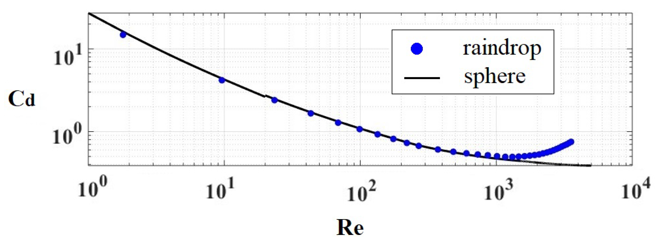
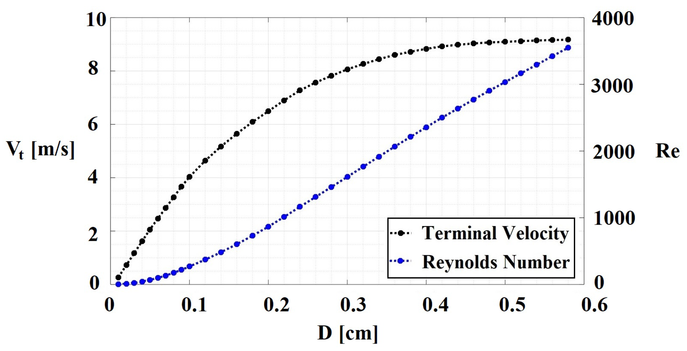
1.3. Drag Coefficients and Terminal Velocities of Water Drops

As we have discussed, small water drops of less than 1 mm in size retain basically a spherical shape, and the drag force on the drop is barely influenced by the regular internal circulation until the Reynolds number reaches around 300. These coincide with the minimum difference in the drag coefficients C d of a rigid sphere (Re ≤ 300) and a water drop smaller than 1 mm in size at its terminal velocity [31], as shown in Figure 1. As Re reaches values larger than 300, water drops begin to oscillate, deformation of the drop is more obvious, and the internal circulation becomes chaotic at higher Re. Accordingly, the divergence in C d intensifies progressively with increasing Reynolds number (larger drops). Terminal velocities, as well as the corresponding Reynolds numbers, for water drops of various sizes are displayed in Figure 2, according to the measurements of Gunn and Kinzer [11].

2. Numerical Methods

We conducted direct numerical simulations of a water drop falling in turbulent flow using the DNS multiphase code FS3D [37]. FS3D solves the incompressible Naiver–Stokes equations. For the description of multiphase flows and the interfaces between immiscible phases, the VOF method [38] using a Piecewise Linear Interface Calculation (PLIC) is applied [39].
The flow field inside a drop and its surrounding air are calculated using the conservation equations for the mass and momentum of incompressible flow,
· u = 0 ,
[ ρ u ] t + · [ ρ u u ] = p + · μ [ u + ( u T ) ] + ρ g + f st .
Here, ρ donates the density, t the time, u the velocity vector, p the pressure, μ the dynamic viscosity and g the gravity vector. The surface tension force fst is modelled with the balanced-force Continuum Surface Force (CSF) method combined with Height Function (HF) curvature technique proposed by Popinet [40]. The pressure field is computed by solving a Poisson equation implicitly, using a multi-grid algorithm [41].
The VOF variable f is used to identify the location of the gas and liquid phases and is defined as:
f ( x , t ) = 1 in the disperse phase , 0 < f < 1 for interfacial cells , 0 in the continuous phase .
The transport equation of the variable f reads:
f t + · [ f u ] = 0 .
To suppress numerical diffusion of the liquid phase, the PLIC method proposed by Rider and Kothe [39] is used to reconstruct the interface after each time step. Within each interface cell, the reconstruction is done by the approximation of a normal vector n of the interface where n = f / f . The position of the reconstructed plane corresponds to the VOF variable f in each interface cell and is solved through iterations [41].
Following the one-field formulation, the material properties of the liquid and gas phase are calculated as follows,
ρ ( x , t ) = ρ l f ( x , t ) + ρ g [ 1 f ( x , t ) ] ,
μ ( x , t ) = μ l f ( x , t ) + μ g [ 1 f ( x , t ) ] ,
where the subscripts g and l indicate the gas phase and the liquid phase, respectively.
The finite volume method based on a MAC staggered grid is employed for the spatial discretisation [42]. Hence, all scalars are stored at cell centres and velocity vectors at cell faces. A first-order explicit Euler scheme is used for the time integration. The maximum time step sizes are restricted by the Courant–Friedrichs–Lewy (CFL) number.
The random spot method of Kornev and Hassel [43] is used to generate anisotropic turbulence, with a freely decaying energy spectrum, within the flow field. The idea is to place a collection of random rotating vortons with a specific inner velocity distribution on the front edge of the inflow area, which then move across the inflow plane at a uniform velocity. An application of the turbulence generator applying this method in FS3D can be found in the work of Zhu et al. [44].

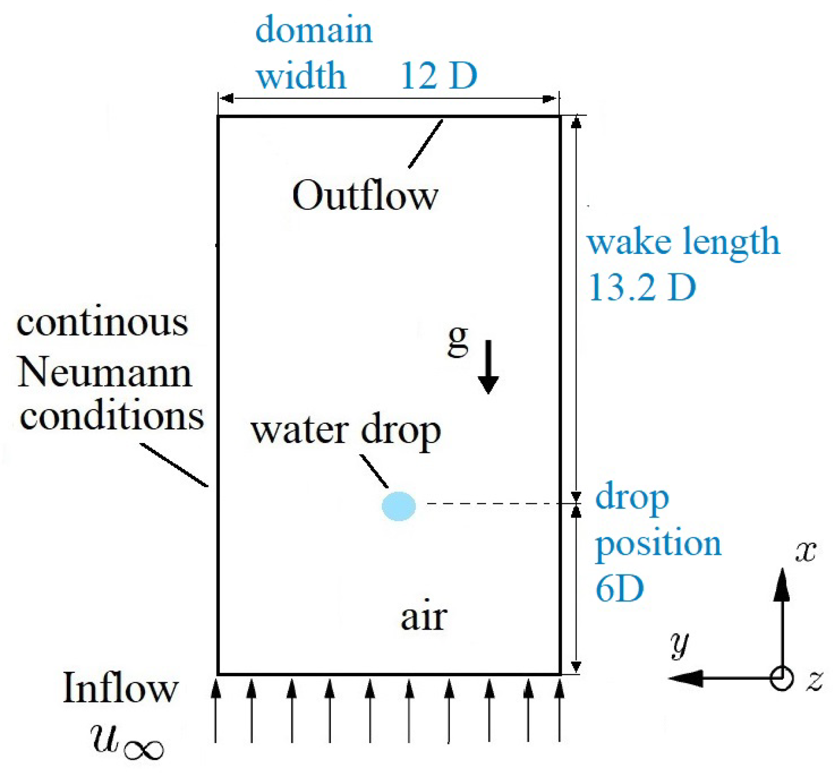
3. Computational Setup

The falling of a water drop in the air flow was computed with an equidistant Cartesian mesh in a 3D rectangular domain. The dimension of the domain is 19.2D × 12D × 12D, with D representing the equivalent drop diameter. The resolution of the drop diameter is about 26.7 cells; the whole domain is resolved by 52.4 × 10 6 computational cells.
Figure 3 shows the computational domain in the form of a 2D slice across the centre of a falling water drop. To minimise the computational effort, a grid that moves in accordance with the falling drop was used. This means that the water drop is positioned at the centre of the yz-plane for the whole falling process with a constant distance of 6D from the inflow and a wake length of 13.2D. The domain width in both z- and y-directions is 12D. This setup was chosen out of four separate series of convergence tests as to guarantee that for all simulation cases, both the grid resolution and the domain size (e.g., wake length, domain width, distance of the drop centre from the inlet plane) have a negligible influence on the fall velocity of a water drop in turbulent air flow (see Appendix A).
As seen in Figure 3, the gravitational acceleration g points in the direction of the negative x-axis. We applied the no slip wall condition at the inflow and continuous boundary conditions (Neumann) on the rest of the domain boundaries. In the case of still air, the air flow at 293.15 K enters the computational domain with a uniform velocity. In the case of a water drop falling across turbulent air flow, the random spot method by Kornev and Hassel [43] was applied for the generation of a turbulent inflow. The grid used is fine enough to resolve the smallest turbulent scales. For a 3 mm water drop falling at its terminal velocity, the ratio between the cell size L c and the Kolmogorov length scale λ k = L t / R e t 3 / 4 is around 2.3 with R e t = ρ air u 2 ¯ L t / μ air , the turbulence length scale L t = 0.75 mm and a turbulence intensity T u = 10%.
In Table 1, the relevant physical properties of the water and air are summarised, with σ , μ and ρ , denoting the surface tension, the dynamic viscosity and the density, respectively.

4. Results

In this section, we present the simulation results regarding how turbulence influences a 3 mm and 2 mm falling water droplet. We will also show that the results for the still air cases match quite well with previous studies, in terms of the terminal velocities, drop oscillation behaviour and wake flow characteristics. In cases of turbulent inflow, we set the turbulence intensity to either 5% or 10% and the turbulence length scale L t to 1/4D or 1/2D.

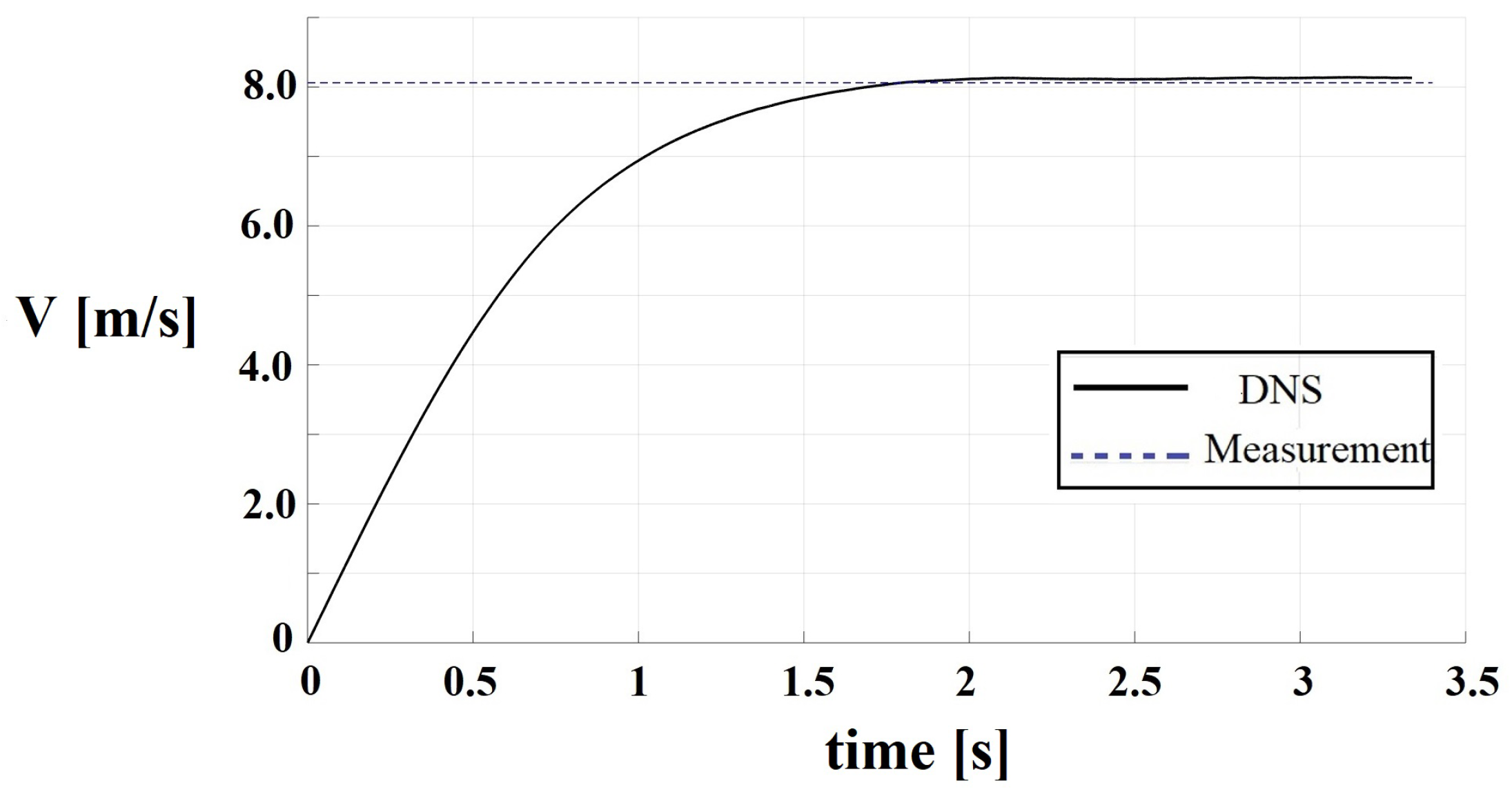
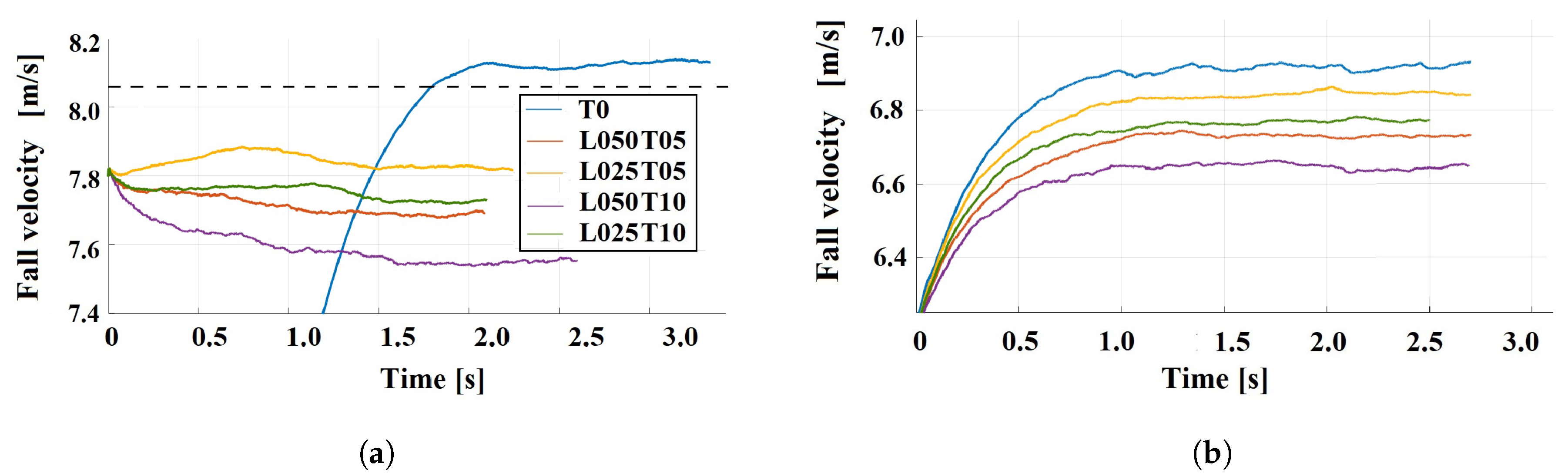
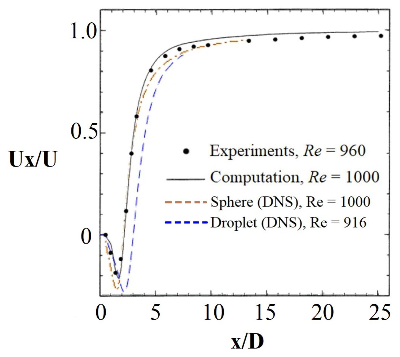
4.1. Terminal Velocity

Table 2 and Table 3 summarise the v t measured by Gunn and Kinzer [11] and the current simulation results from FS3D. In Table 3, with regard to the name of each test case, D indicates the equivalent drop diameter, L the ratio of the turbulence length scale and the drop diameter and T the turbulence intensity. Hence, D2L050T10denotes, for instance, the case of a 2 mm water drop falling in a turbulent surroundings. At the inflow area, the turbulence length scale is set to 1 mm, and the turbulence intensity is 10%.
Results from the simulations were all averaged over a time period of 0.5 s after the fall velocity of the drop stabilised. The trend for v t of both the 3 mm and 2 mm water drops matches well with the measured values, as in Table 2 and Table 3.
Figure 4 illustrates the v t of a 3 mm water drop according to Gunn and Kinzer [11], along with the evolution of the fall velocity of the simulated 3 mm water drop that falls in still air.
Figure 5 displays the fall velocity of the water drop over time in all simulation cases. In most cases (except D3T0), the water drop was initially set to fall at a velocity close to the expected v t . This approach saves the computational time required for a falling water drop to finally stabilise at its v t .
In turbulent air flow, v t of both water drops is reduced. The fluctuations of the drop fall velocities are comparable in all conducted cases. The maximum reduction in v t reaches 7.1% and occurs in the case D3L050T10. The results in Table 3 suggest that in the range under investigation, a larger turbulence length scale and higher turbulent intensities at the inflow area tend to cause a stronger reduction of v t , as well as a more intense rise in C d . In addition, in terms of v t , turbulence has more influence on the 3 mm water drop with a higher Re than on the 2 mm water drop.

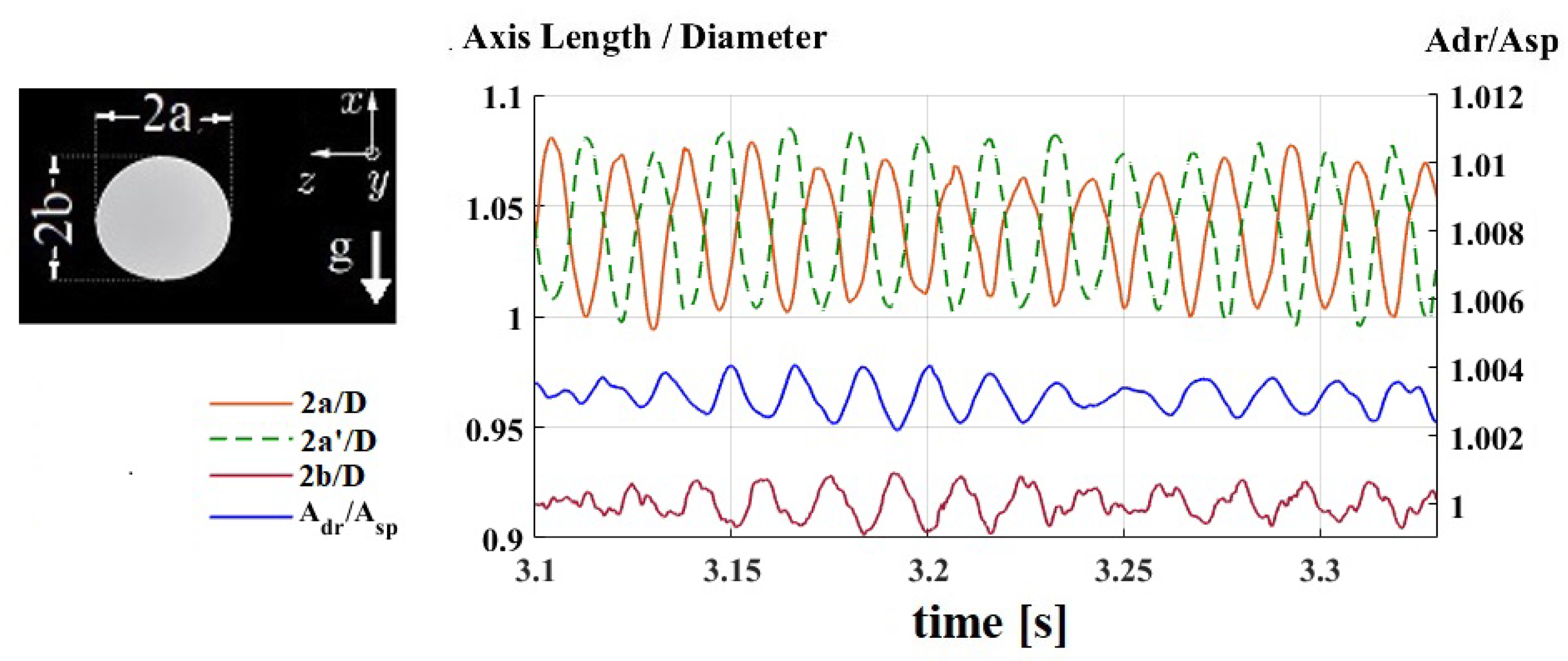
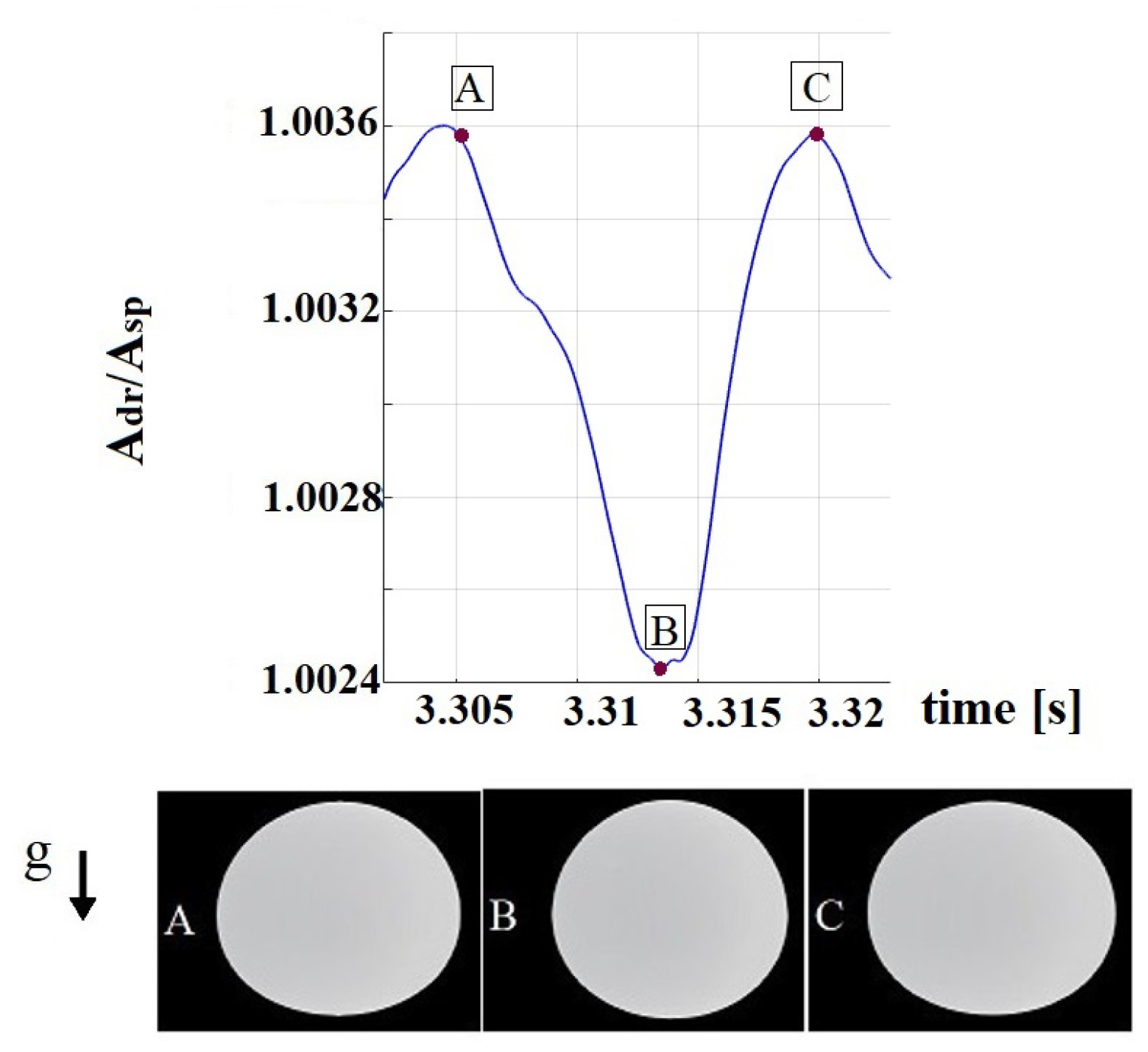
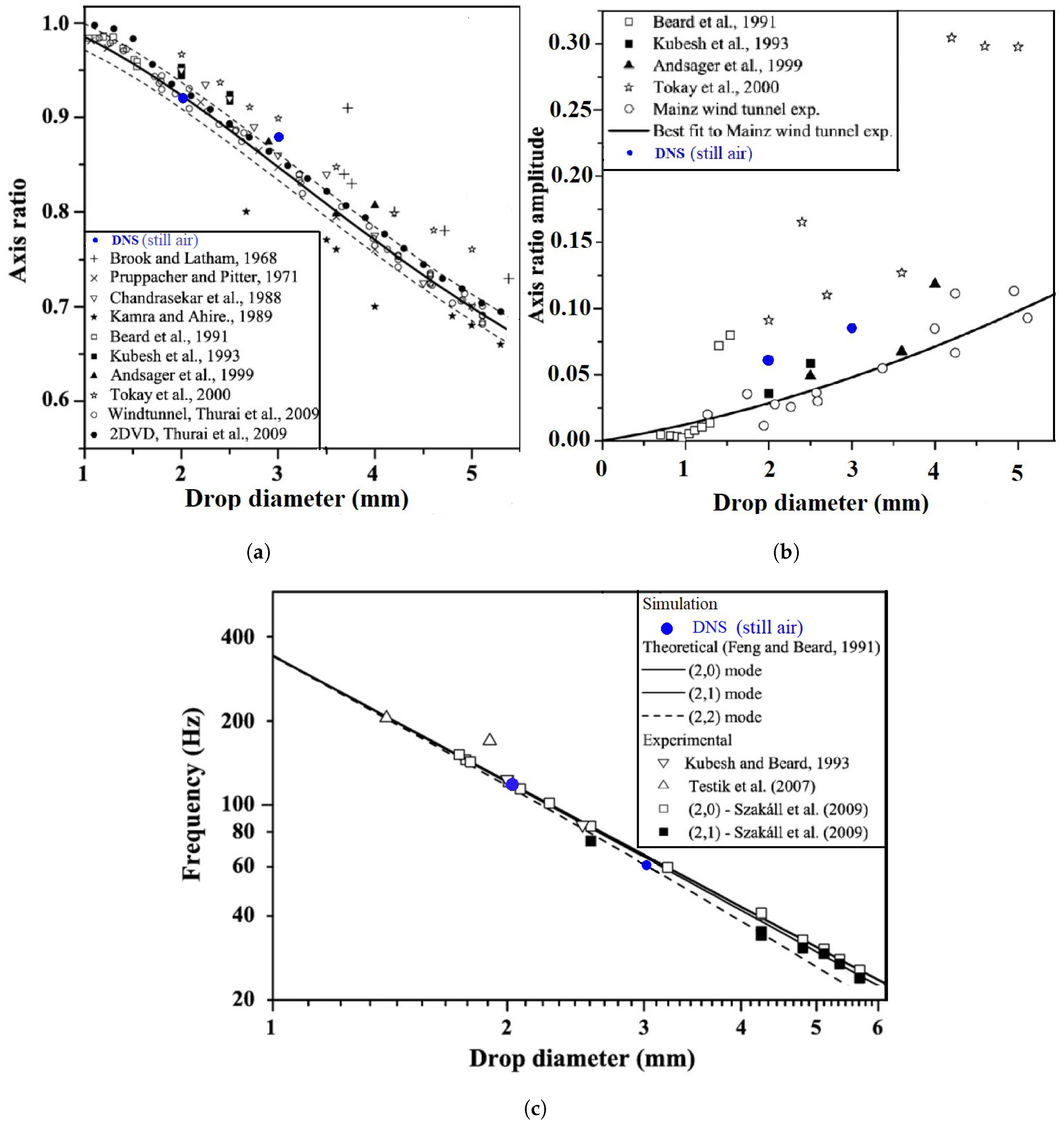
4.2. Drop Shape Deformation and Drop Oscillation
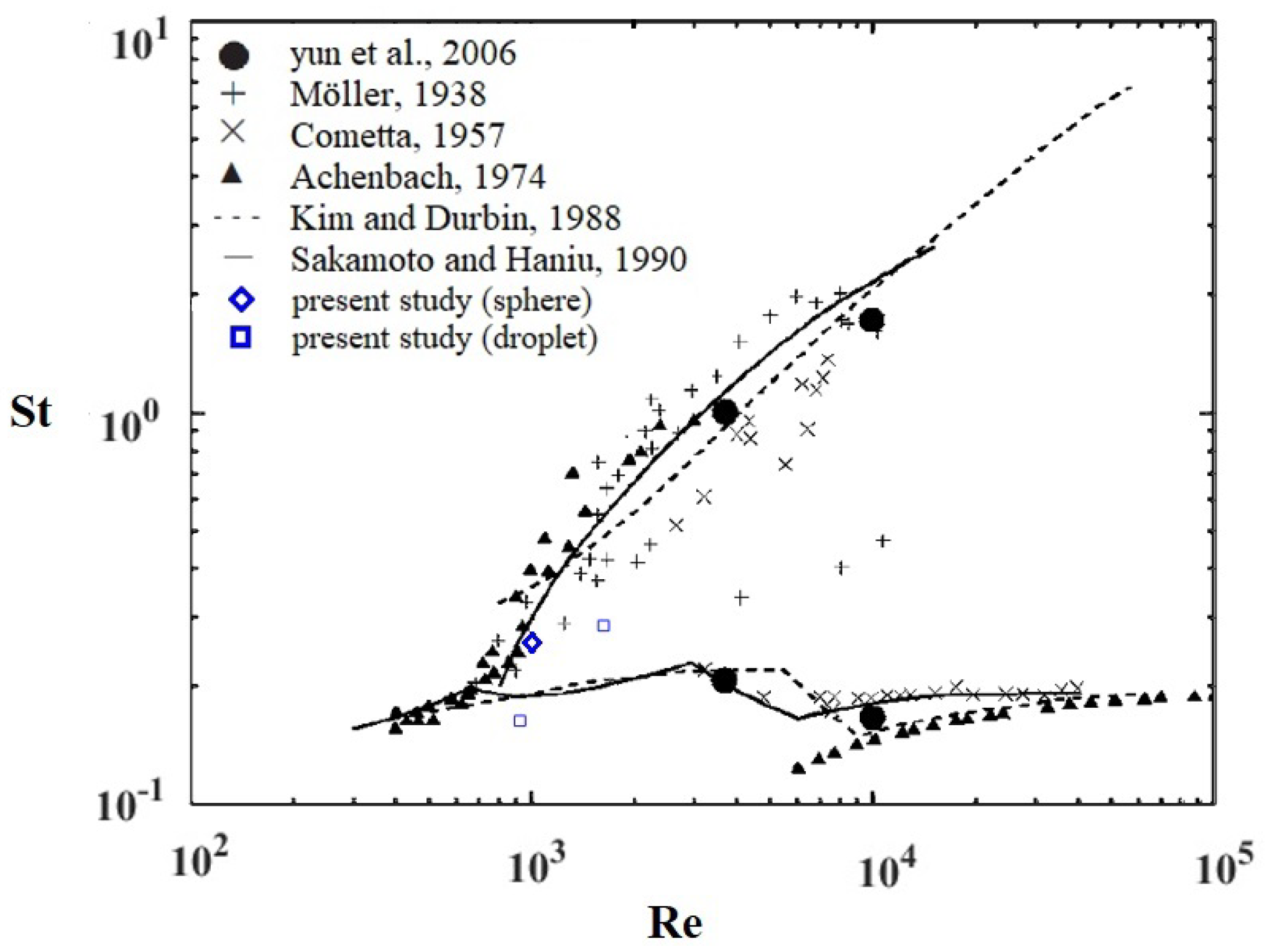
Figure 6 shows an example of the temporal variation of the surface area ratio A d r / A s p , the normalised major (horizontal or lateral) axis lengths 2 a / D , 2 a / D and minor (vertical) axis lengths 2 b / D of a 3 mm water drop falling in stagnant air over several oscillation periods. A d r and A s p denote the surface area of a drop and that of a sphere of equivalent diameter, respectively. 2 a / D was measured in the y-direction (orange curve) and 2 a / D in the z-direction (green curve). The variation in A d r / A s p and 2 b / D fits well. As the minor axis reaches its minimum, the drop surface area reaches its maximum and vice versa.
In Figure 7, we demonstrate the surface deformation across one oscillation period of a 3 mm water drop falling in still air. During the falling process, the water drop is flattened and takes an oblate shape. The deformation of the water drop at the instants A, B, and C displays a good match with the photos for the falling rain drops of 2.7 mm and 3.45 mm taken by Pruppacher and Beard [34]. In addition, we compared our results regarding the oscillation frequency, the axis ratio amplitude and the mean axis ratio with the measurements and theoretical models from previous studies (Figure 2, Figure 3 and Figure 4 from the review of Szakall et al. [30]) and found a quite good agreement for the simulated 3 mm and 2 mm water drops that fall in still air (see Appendix B).
Table 4 summarises the time-averaged drop axis ratio, horizontal axis length 2 a ¯ , oscillation frequency and the temporal axis ratio amplitude for all conducted cases. Turbulence exerts only a minimum effect on both the drop axis ratio and horizontal axis length. The largest increase in both parameters is less than 1%, which occurs in the cases D3L050T10 and D3L050T05. Thus, we suggest that the mean effect of 2 a ¯ on the pressure drag is invariant to moderate turbulence. In turbulent surroundings, the increase in the axis ratio amplitude is obvious particularly in cases such as D3L050T10 and D2L050T10, both with an increase of over 50%. This means a higher temporal variation of the oscillation amplitude for a water drop that travels across a flow with a larger turbulence length scale (comparable to the size of the drop) and higher turbulence intensity. However, this large variation in the oscillation amplitude was not sufficient for an abrupt fall velocity variation (see Figure 5). In turbulent air flow, the oscillation frequencies either increase slightly or remain at the same values. The increase is more obvious for the cases with a flow field of a larger turbulence length scale and higher turbulence intensity.

4.3. Flow Field

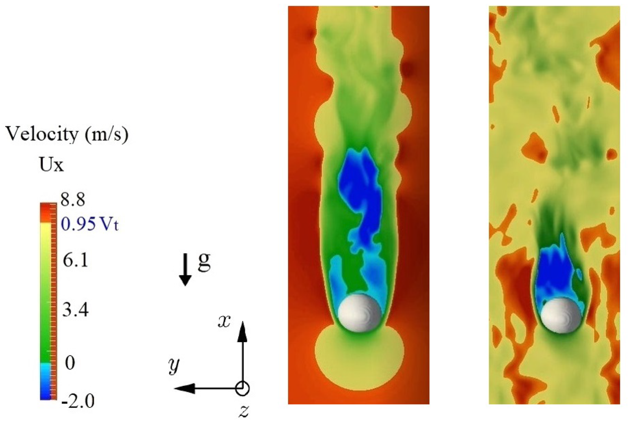
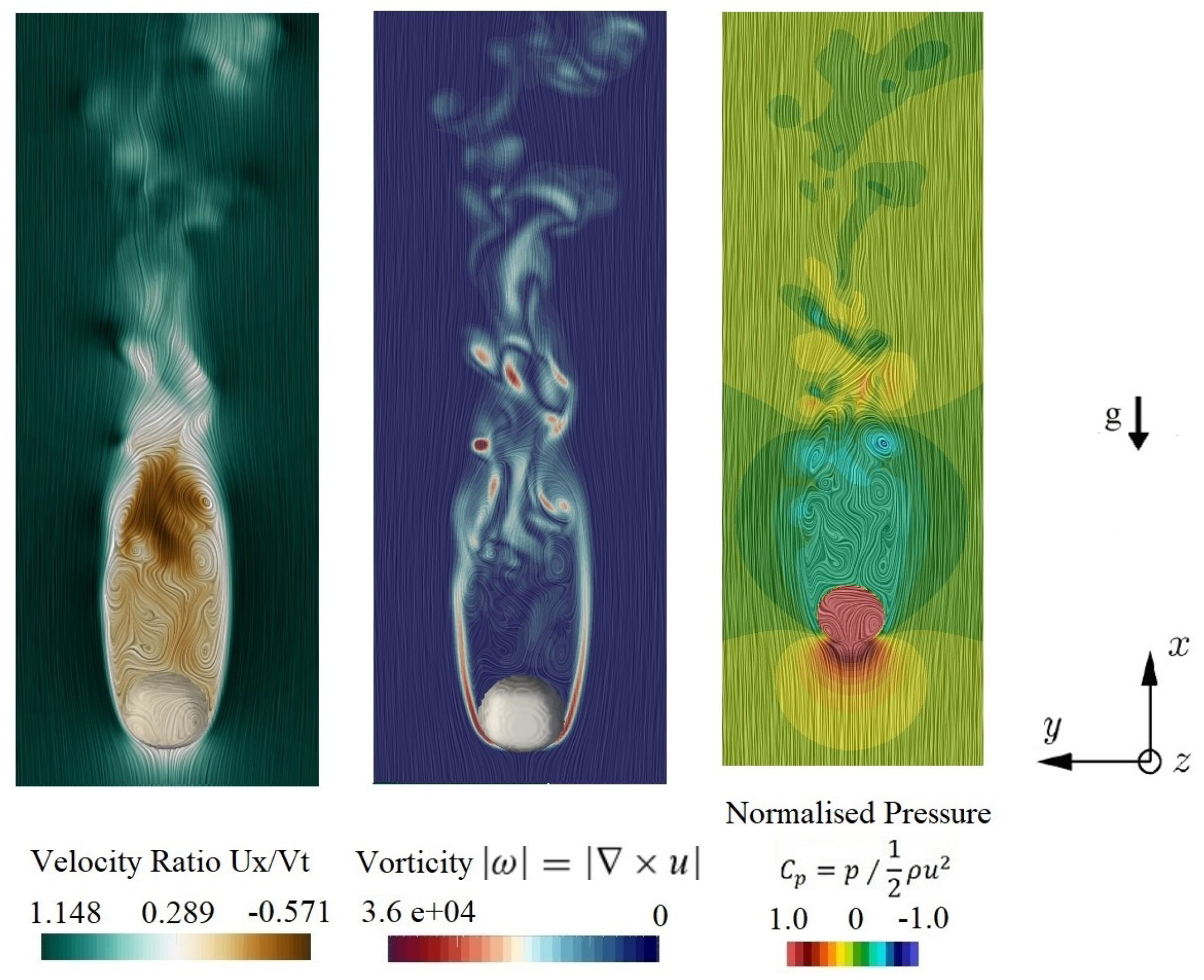
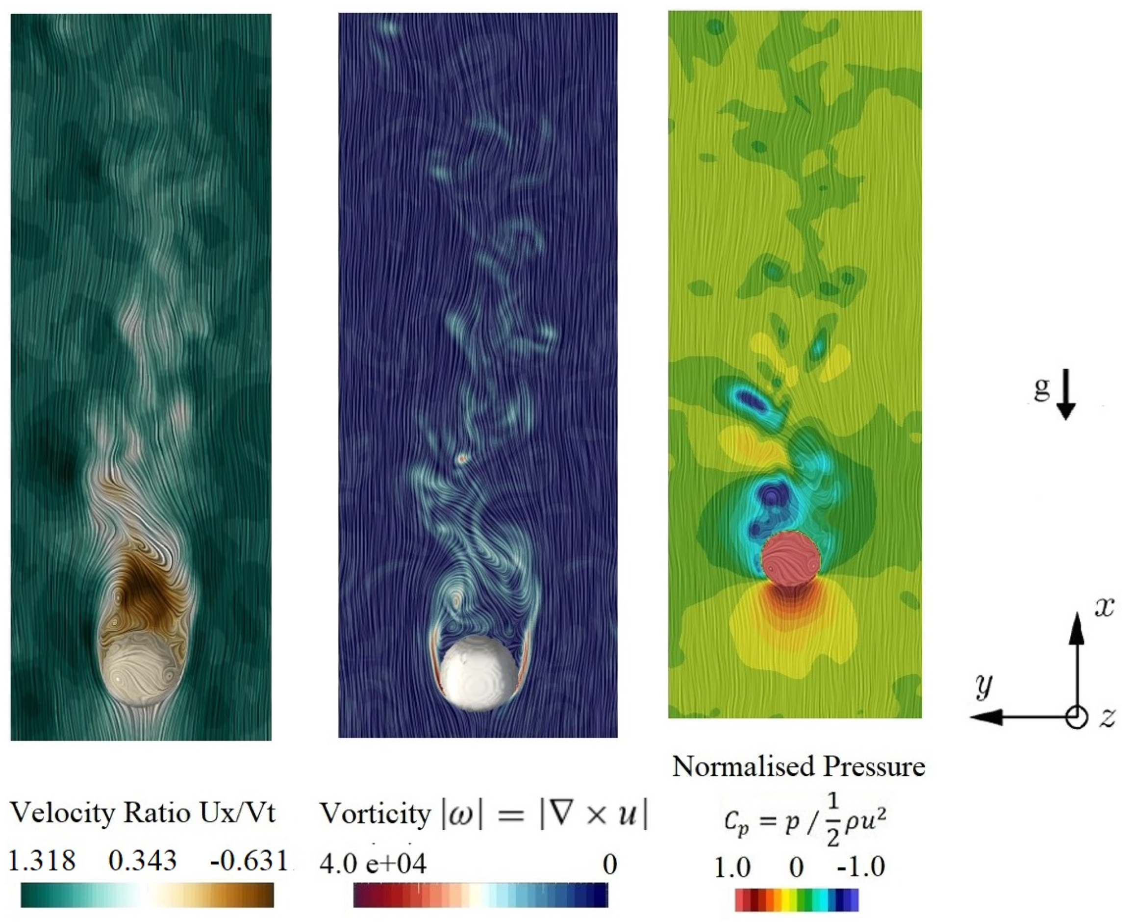
4.3.1. Instantaneous Flow

Figure 8 compares the instantaneous velocity field of a 3 mm water drop falling in stagnant air (D3T0) with that in turbulent air flow (D3L050T10). The flow separates from the drop surface near a point at which the velocity in the stream-wise direction U x turns from a positive to a negative value. This is illustrated by the colour change from green to blue near the drop surface. The boundary layer thickness is indicated by the change in colour from red to yellow near the drop surface, which occurs at about 0.95 v t . Downstream of the drop base, the blue colour, where U x adopts negative values, characterises the wake recirculation. As shown in Figure 8, the turbulent surroundings do not seem to have an obvious influence on both the flow separation point and the boundary layer thickness, but it has a strong influence on the wake recirculation area. The water drop falling in stagnant air shows a recirculation area that is about twice the length of that of the water drop in turbulent air flow.
A comparison of the instantaneous flow field including the velocity field along with the streamlines, the vorticity field and the pressure field between both cases is depicted in Figure 9 and Figure 10. The vortices shown in both figures visualise the wake recirculation region of the water drop, which ends where the streamlines merge. The colour change downstream the wake recirculation clearly illustrates the recovery of flow velocity in both cases, where the tortuosity of the streamlines is weakened.
Compared to the case in stagnant air, the streamlines in the case D3L050T10 are crooked in the inflow region and far field. In both cases, the vorticity magnitudes increase significantly on the front half of the drop surface, which then decrease continuously along the shear layers. At the rear end of the recirculation region, the flow demonstrates high pressure losses and strong vorticity. We explored the vortex shedding process of both cases and discovered that the turbulent surroundings triggers an earlier onset of the shear layer instability, as well as a more irregular, unsymmetrical and much smaller wake recirculation region. In the case D3L050T10, the vortex is formed near the drop surface immediately after the flow separates. In the case of stagnant air, the main vortices within the shear layer mostly start to form at around 1.0D downstream of the flow separation point. We observe increasing pressure losses at these vortices as they travel downstream. The detachment of a vortex within the shear layer can be recognised by the saddle point of the streamlines beside the vortex, where the pressure loss and the vorticity magnitude in the vortex core reach local maxima. With a drastic reduction in the size of the wake recirculation, the strong pressure loss draws nearer to the base of the water drop. The base suction pressure −Cpb is thus higher in the case D3L050T10 than that in the still air case. Similar changes in the near wake region were found for the cases with a less intense turbulent inflow, as well as in the cases with the 2 mm water drop. Hence, we think that this might be one potential influential factor that relates to the reduction of the terminal velocity of a water drop.

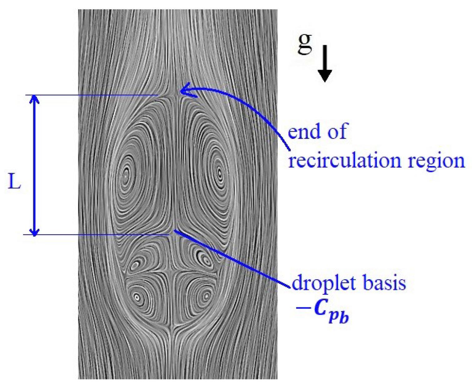
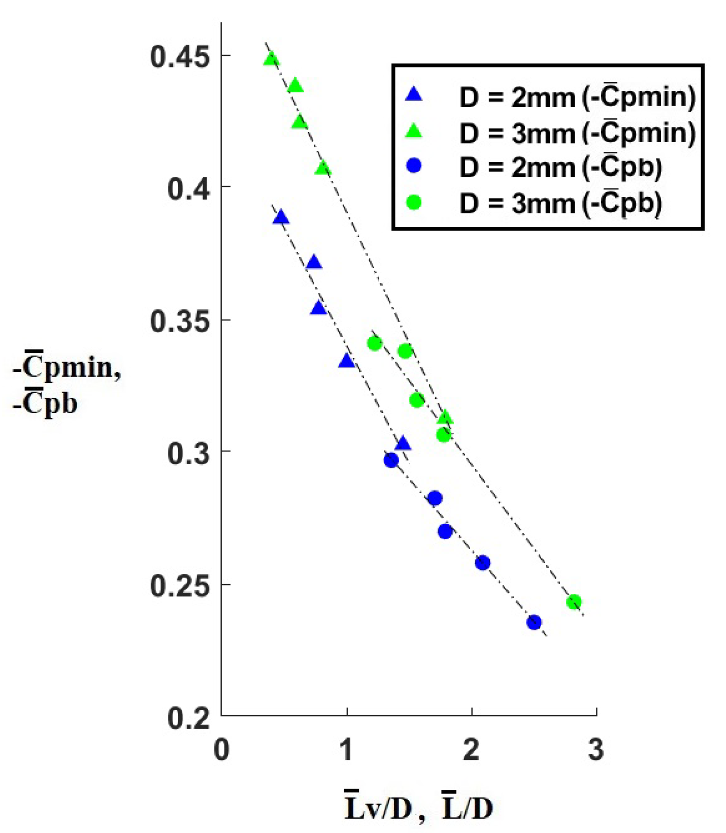
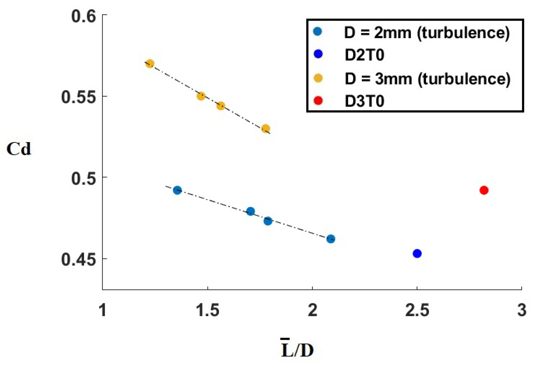
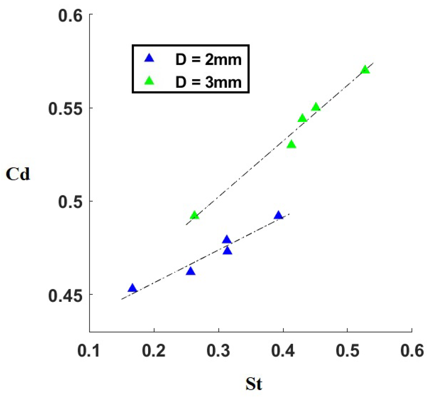
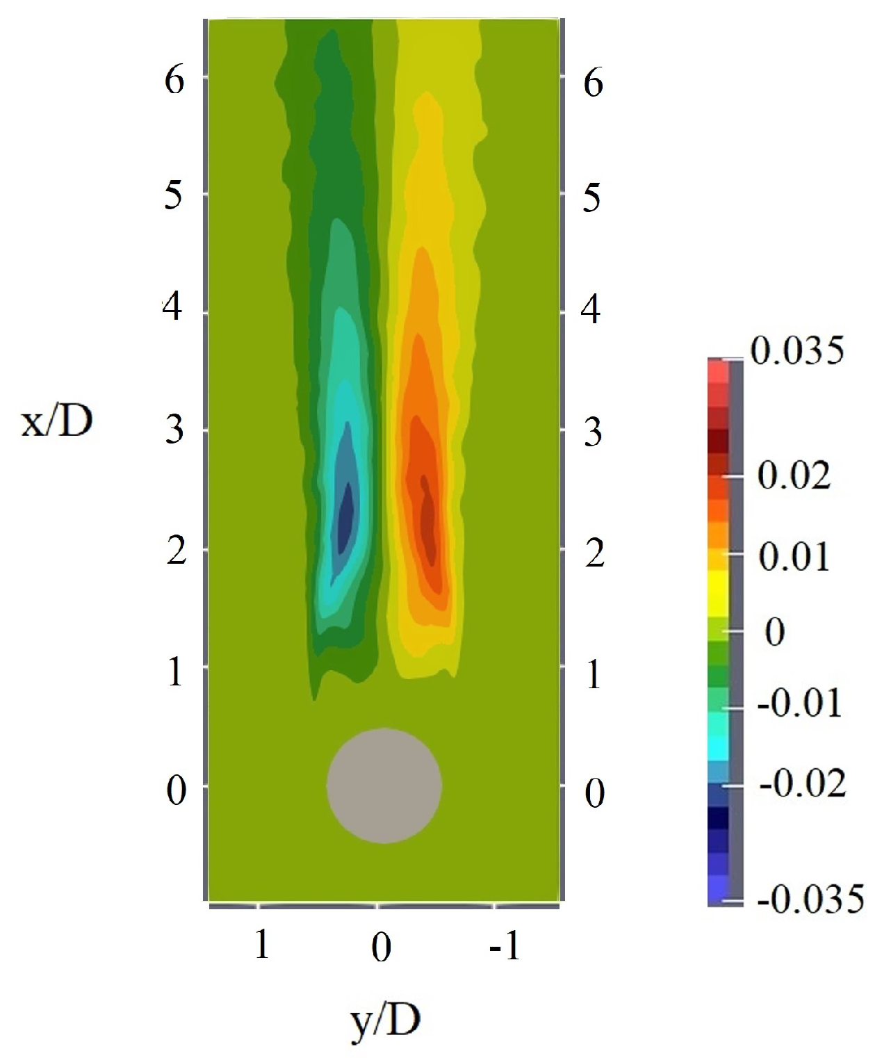
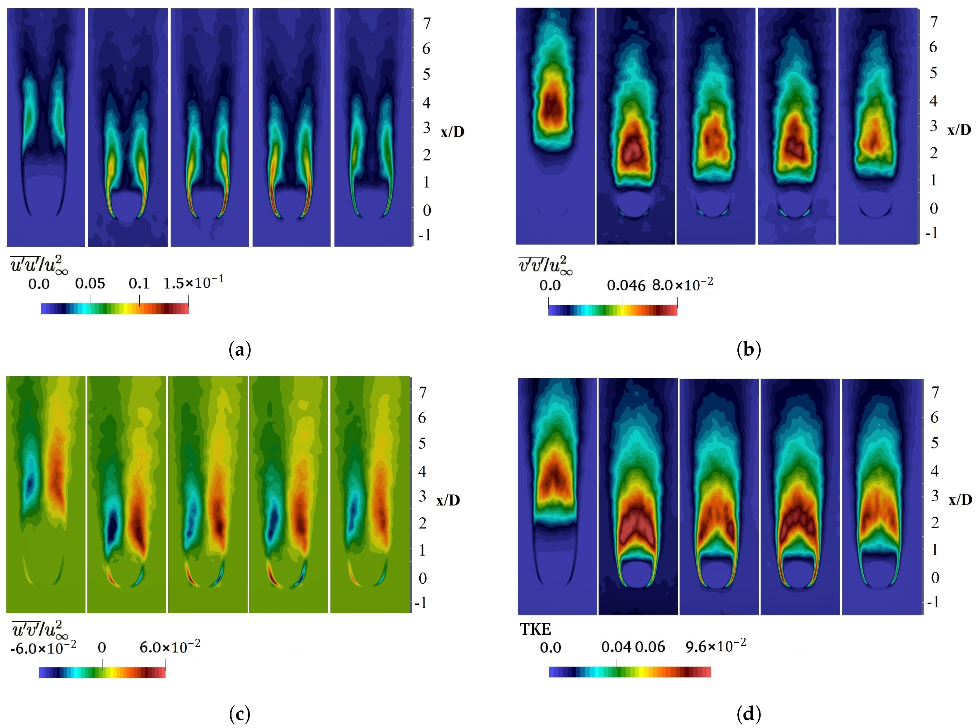
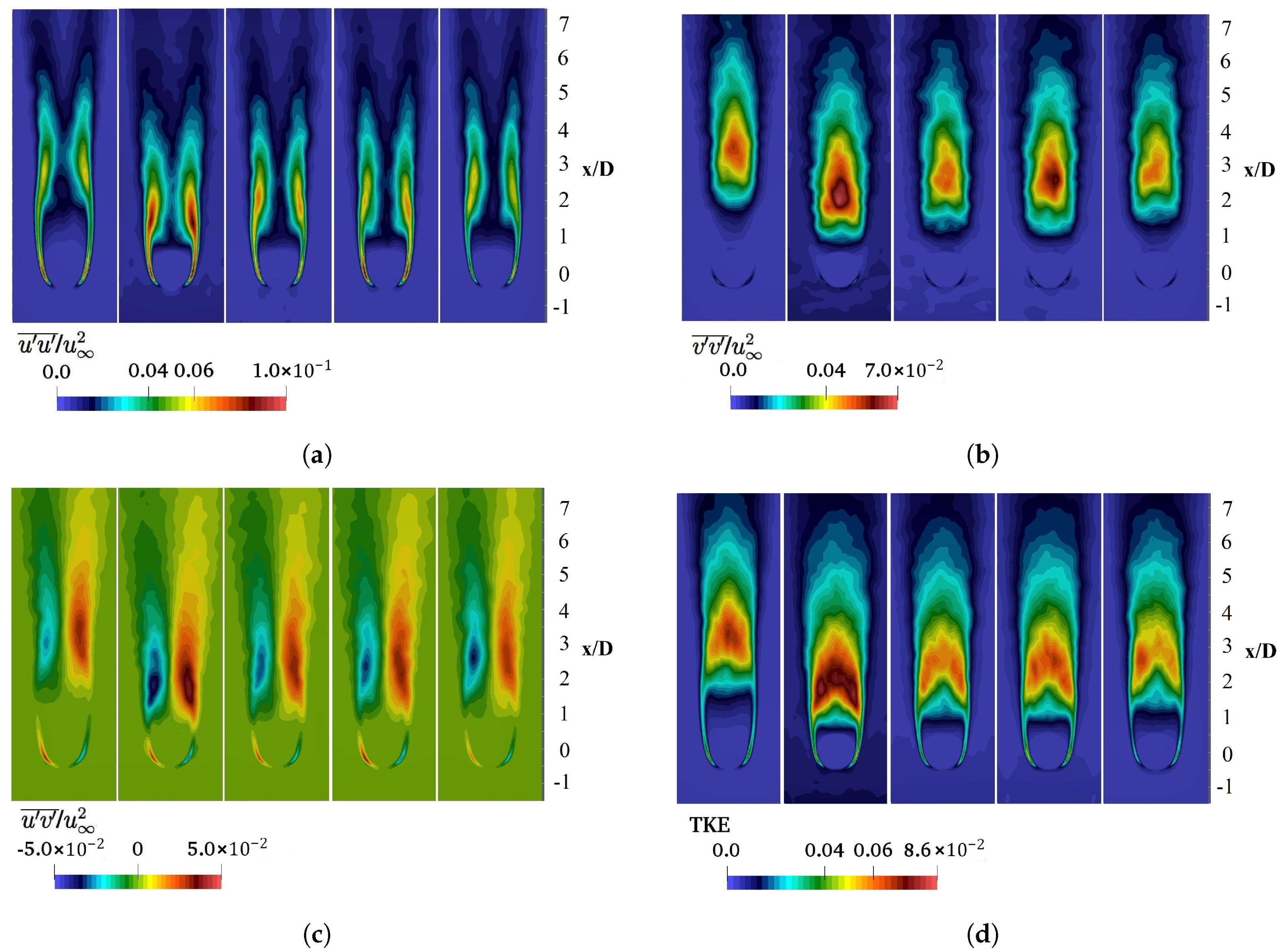
4.3.2. Mean Flow Parameters

In this section, we present the quantitative details of the flow field characteristics. We will first show that our results for the still air case are in good agreement with previous studies.
Table 5 presents a summary of the time-averaged flow parameters, which include the flow separation angle θ ¯ s , recirculation bubble size L ¯ / D (see Figure 11), base pressure coefficient − C ¯ pb = ( p b p ) / ( 1 / 2 ρ u 2 ) , vortex formation length L ¯ v / D , minimum pressure coefficient on the wake axis − C ¯ pmin and the Strouhal number S t = f r D / U . Here, p b denotes the time averaged pressure at the droplet basis and f r the vortex shedding frequency.
To attain converged statistics, we averaged the flow field of the 3 mm and 2 mm water drops with results from 400 time steps for a time period of 0.28 s and 0.2 s, respectively. This is equivalent to around 760 D / U time units and 16.5 drop oscillation periods in the case D3T0 and around 690 D / U time units and 23 oscillation periods in the case D2T0. θ ¯ s was calculated starting from the flow stagnation point. Four separation points from the two symmetry planes (xy-plane, xz-plane) were used for the averaging. L ¯ / D and L ¯ v / D were both measured along the wake centre-line, starting from a distance of the drop radius from the drop centre. The recirculation region terminates where the time-averaged stream-wise flow velocity U x reaches zero; the vortex formation region ends with the same position of − C ¯ pmin . We estimated the Strouhal numbers by observing the vortex shedding process in the shear layer over a time period of 180 D / U (see Section 4.3.1).
To the best of our knowledge, there exists no measurement data for the flow characteristics (e.g., flow separation, size of the recirculation bubble) of a water drop at Re ≈ 1000. Since both the 3 mm and 2 mm water drops still retain a sphere-like shape in spite of the surface deformation, we may expect the flow in the near wake of a sphere to be similar to that of a water drop at the same Re. Hence, we conducted the simulation of a sphere falling in air with Re = 1000 for the validation. The computation was done using FS3D with a recently developed method for arbitrarily-shaped rigid bodies [45], which was specifically designed to account for the flow velocity within each interface cell of a rigid body.
The simulated time-averaged flow separation occurs at 101.7 from the stagnation point of the sphere, and the length of the recirculation area is found to be 1.71D. Both values match very well with the results from Tomboulides and Orszag [46]. According to their work, the flow separates at 102 , and the length of the recirculation region is about 1.7D. In the case D2T0 (Re ≈ 1000), the flow separation occurs earlier on the drop surface with θ ¯ s = 90.6 . We suspect the deformation of the water drop to be one of the main reasons resulting in an earlier onset of the flow separation. Note that, during the simulation, the water drop displays a minimum shift of the drop centre relative to its original position through the falling process. Since the calculation of the separation angle is based on the original position of the drop centre, this has brought some uncertainties. We estimated the shift of the water drop through overlapping the time-averaged pressure distribution of the drop onto the contour of a 2 mm sphere and found an uncertainty of + 2.3 in the separation angle, meaning that in the case D2T0, the flow separation may take place at an angle of up to 92.9 .
To validate the velocity field in the near wake region, we compared the stream-wise velocity U x /U on the wake centre-line with previous simulation results (Re = 1000) from Tomboulides and Orszag [46], as well as with the experimental data (Re = 960) by Wu and Faeth [47]. Figure 12 shows a good agreement between the results from FS3D and those from the previous studies. The length of the wake recirculation bubble L ¯ / D of the 2 mm water drop is 2.5D, which is about 47% longer than that of the sphere. This matches well with the displacement of U x /U in the downstream direction, as shown in Figure 12. In the case of a falling water drop, the drop surface deformation and drop oscillation will have some influence on the length and width of the wake recirculation region. Furthermore, we suspect an increase in the width of the shear layer, which wraps around the water drop, as a result of the earlier onset of flow separation. This should eventually lead to a larger L ¯ / D . The large-eddy simulation (LES) conducted by Yun et al. and the DNS by Rodriguez et al. [28,48] show comparable results for L ¯ / D and θ ¯ s in the case of a flow over a sphere at Re = 3700. L ¯ / D was predicted to be 2.622 and 2.28 and θ ¯ s to be 90 and 89.4 , according to Yun et al. and Rodriguez et al., respectively.
Through our observation, the Strouhal number S t of the 2 mm water drop falling in still air was found to be significantly lower than that of the 3 mm water drop. Moreover, the vortex shedding process of these two cases has been noted to be slightly different. In the case of the 3 mm water drop, vortices are often observed travelling further downstream after detaching from the shear layer, while in the case of the 2 mm water drop, vortices are most likely to be drawn to the centre-line of the wake after their detachment, which then disappear shortly after. A comparison of S t for the wake of simulated water drops and that of spheres at different Re is shown in Figure 13. S t of the simulated sphere obtained through observation is 0.26 and lies between the low-mode S t associated with the large-scale wake instability and the high-mode S t for the small-scale shear layer instability measured in the previous studies. At the same Re, S t appears to be higher in the rigid sphere case than in the case of a water drop. Magarvey and Bishop [49] studied the wake of a drop in a liquid system with Re ranging from 350 to 500. They also reported the S t of the drop, which were lower than those of a rigid sphere.
Turbulence has a great influence on the vortex shedding process in the shear layer, as well as on the flow characteristics in the near wake of the water drop. In turbulent cases, the formation and shedding of vortices take place at an earlier point in the shear layer and at higher frequencies. Cases D3L050T10 and D2L050T10 exhibit the earliest vortex formation near the drop surface; cases D3L025T05 and D2L025T05 display the lowest level of the displacement of vortex formation in the upward direction relative to the still air cases.
As in Table 5, the turbulent surroundings cause a backward movement of the flow separation points θ ¯ s , an increase in the critical wake flow parameters S t , − C ¯ pb and − C ¯ pmin , as well as a shortening in L ¯ v / D and L ¯ / D . It is clear that in stronger turbulence conditions, where L t = D/2 or T u = 10% at the inflow, there is a more intense delay of the flow separation and a stronger rise in S t .
Changes in the other four wake parameters all display a similar tendency that the reduction of L ¯ v / D and L ¯ / D , as well as the corresponding increase of − C ¯ pmin and − C ¯ pb become more significant in stronger turbulence conditions, which is consistent with the rise in C d . Figure 14 displays the strong relation between these four parameters amongst all simulation cases. As illustrated in the figure, the reduction in L ¯ v / D and L ¯ / D corresponds to a proportional increase in − C ¯ pmin and − C ¯ pb , respectively. More interestingly, for each case, the ratio between − C ¯ pmin and − C ¯ pb falls between 1.29 and 1.33, with a maximum ratio discrepancy of around 3%. In addition, the figure indicates less impact from the turbulence on the 2 mm water drop than on the 3 mm drop, where the shortening of L ¯ / D ranges from 16.4% to 45.6% with the 2 mm drops; with the 3 mm drops, from 37.2% to 56.4%. The increase in − C ¯ pb lies between 9.6% and 26% in the 2 mm drop case and between 26% and 40% in the 3 mm drop case.
Figure 15 illustrates a strong connection between L ¯ / D and C d . In the case of turbulent surroundings, C d increases linearly with the decrease of L ¯ / D . This however does not occur in the still air case, where the C d of both 3 mm and 2 mm water drops is located higher than the elongation of the dotted lines. This indicates that other factors, which tend to reduce C d in the case of a turbulent surroundings, may exist, and especially so for a 3 mm water drop.
In Figure 16, C d of the simulated water drops is plotted as a function of S t . These data points lie close to the straight line with a slope of 0.299 (3 mm drop) and 0.176 (2 mm drop).
In the following section, we examine the distribution of the time-averaged Reynolds stresses (e.g., the stream-wise Reynolds stress u u ¯ / u 2 , the transverse Reynolds stress v v ¯ / u 2 and the Reynolds shear stress u v ¯ / u 2 ) and turbulent kinetic energy T K E in the flow field, as these further reveal the influence of turbulence on the shear layer and wake instabilities, which are closely associated with the vortex shedding process, recirculation in the near wake, as well as the base suction pressure.
Figure 17 displays u v ¯ / u 2 of flow past a sphere at Re = 1000 simulated with FS3D. The result is in good agreement with that computed by Poon et al. [50].
Figure 18 and Figure 19 depict the distribution of u u ¯ / u 2 , v v ¯ / u 2 , u v ¯ / u 2 and T K E for the 3 mm and 2 mm water drops, respectively. Compared to the sphere case, the Reynolds stress near the drop surface is increased, and we think that this relates more to the dynamic drop oscillation.
For all conducted cases, the peak value of u u ¯ / u 2 appears at the shear layer and lies stream-wise between the end of the vortex formation region and wake recirculation region. Regions of stronger v v ¯ / u 2 are seen near the centre-line of the wake. The maximum of v v ¯ / u 2 is located directly behind the end of the recirculation area. The field of v v ¯ / u 2 and that of w w ¯ / u 2 (not displayed) downstream the drop base are found to be quite similar. The contours of the Reynolds stresses, in accordance with the shortening of the wake recirculation area, are thus shifted upwards closer to the drop base. Cases D3L050T10 and D2L050T10 display the largest displacement upwards for the 3 mm and the 2 mm drop case, respectively. In addition, in the cases of higher turbulence intensities and a larger turbulence length scale, T K E reaches higher values at the shear layer at an earlier stage due to stronger velocity fluctuations between the shear layer and the free stream. The stronger and faster increase in the T K E level corresponds to a more obvious displacement of Reynolds stress components, as well as a more significant reduction in L ¯ / D , as seen in Figure 18 and Figure 19.
In cases D3L050T10 and D2L050T10, T K E reaches the highest value of around 0.1 and 0.08 at 0.85–1.1D and 1.15–1.25D at the shear layer downstream of the drop base, respectively. This implies that there is still room for a further reduction of L ¯ / D in the case of a stronger turbulent air flow, where C d continues to increase until the boundary layer and the shear layer become fully turbulent and drag crisis sets in.

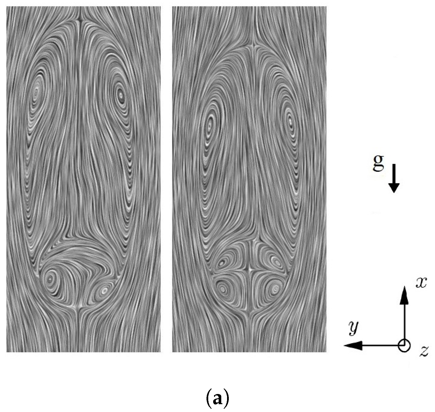
4.4. Internal Circulation

Figure 20a depicts the time-averaged streamlines for the 3 mm and 2 mm drop falling in stagnant air. The symmetrical wake recirculation area in both cases indicates good statistical convergence. In contrast to the 3 mm water drop, the 2 mm water drop is less flattened; the recirculation area appears to be shorter and narrower. Inside the 3 mm water drop, the streamline pattern illustrates a pair of well-developed circulation. The flow inside the 2 mm water drop displays a pair of well-organised secondary recirculation opposing the primary circulation.
Instantaneous streamlines of the 2 mm drop show that as the drop oscillates and gets more flattened with increasing major axis length, the core of the secondary recirculation is shifted towards the drop surface near the flow separation. As the major axis reaches its maximum, the secondary recirculation is disrupted and tends to break down. Inside the 3 mm water drop, the opposing circulation rarely appears and disappears shortly after as a result of the mixing effect of the near-wake flow. Figure 20b,c displays an example of the streamlines for 3 mm and 2 mm water drops at different time steps, respectively.

5. Conclusions

The present work investigates how the terminal velocity of a 2 mm (Re ≈ 900) and 3 mm (Re ≈ 1600) water drop are influenced by the turbulent surroundings by means of direct numerical simulations. We examined the turbulence effects on both the dynamic drop oscillation and flow field characteristics. At the inflow area, the turbulence intensity T u was set to vary between 0%, 5% and 10%; with the turbulence length scale L t between a quarter or a half of the drop diameter. In the cases of still air, the simulated terminal velocity, as well as the drop oscillation behaviour (e.g., the drop oscillation frequency, drop axis ratio and axis ratio amplitude) are in good agreement with the results from previous studies. The characteristics of the flow field were validated through the DNS of the flow over a rigid sphere at Re = 1000. The flow separation point, the size of the wake recirculation region, the Strouhal number, the stream-wise velocity along the centreline of the near wake, as well as the Reynolds shear stresses all match well with previous studies.
The DNS results show a decrease in the terminal velocities v t for both water drops falling in turbulent air flow. The drag coefficients C d of both water drops increase. A stronger turbulent air flow (higher T u and a larger L t ) at the inflow region results in a greater decrease in v t .
The study of the drop oscillation behaviour and the characteristics of flow over the water drop reveals that the rise of C d is strongly associated with the decrease in the length of the wake recirculation region L ¯ / D , as well as the rise in the base suction coefficient − C ¯ pb . In terms of the drop surface deformation, the time-averaged drop axis ratio and length of the drop major axis are barely influenced by the turbulence. In the cases of stronger turbulence surroundings, the increase of the drop oscillation frequency becomes obvious; the rise in the axis ratio amplitude becomes much more significant. However, the fluctuations of the drop fall velocities are still comparable in all simulation cases. A great impact from the turbulent air flow on the near wake flow region is revealed by the instantaneous streamlines, which clearly display the increased irregularity and shortening of the recirculation area in the near wake region. Accordingly, the pressure loss at the rear end of the wake recirculation is shifted upstream.
Regarding the influence of the turbulence on the statistical flow parameters, we found an increase in the flow separation angle, base suction pressure − C ¯ pb , minimum pressure coefficient − C ¯ pmin and Strouhal number S t and a decrease of the wake recirculation length L ¯ / D and vortex formation length L ¯ v / D . The impact from a stronger turbulent air flow is more intense on these parameters. Strong correlations between the wake parameters − C ¯ pmin , − C ¯ pb , L ¯ v / D and L ¯ / D are displayed. For all simulation cases, the ratio between − C ¯ pmin and − C ¯ pb lies near a constant value (around 1.3). The reduction in L ¯ v / D and L ¯ / D corresponds to a proportional increase of − C ¯ pmin and − C ¯ pb .
Furthermore, in the cases of turbulent surroundings, C d increases linearly with a decrease of L ¯ / D . The turbulent air flow results in an earlier and more frequent vortex shedding. The increase in the Reynolds stresses, as well as in the turbulent kinetic energy T K E takes place earlier at the shear layer and is more significant in the cases of stronger turbulent ambient flow. In accordance with the shortening of the wake recirculation area, the contours for the shear stresses and T K E are shifted upwards closer to the drop base.
In addition to the above-mentioned observations, the time-averaged streamlines display a pair of well-organised circulation inside the 3 mm drop and an extra pair of secondary recirculation inside the 2 mm drop in the still air case.
While the current study involves only cases with a limited range of turbulence levels, it is shown that with stronger turbulent air flow, there is still room for a further increase in T K E at the shear layer, shortening of the recirculation area and consequently an increase of C d until the drag crisis sets in. Regarding the simulation results from FS3D, a couple of interesting questions remain unanswered. These include the limit of L ¯ / D , L t and T u for the presence of drag crisis, the impact of ambient turbulence on the drag and the wake flow of a smaller falling water droplet (with a lower Re). Whether the linear relation between C d and L ¯ / D still holds with stronger turbulent air flow also requires further investigations. In addition, it remains to be explored whether or at which turbulence level the influence of the internal circulation/recirculation on the near wake would become strong enough to affect the fall velocity of a drop.

Author Contributions

Conceptualization, W.R. and J.R.; software, W.R. and J.R.; investigation, W.R.; methodologies, J.R.; validation, W.R. and J.R.; formal analysis, W.R.; data curation, W.R. and J.R.; visualization, W.R.; writing, original draft preparation, W.R.; writing, review and editing, W.R., J.R. and B.W.; supervision, J.R. and B.W.; project administration, J.R. and B.W.; funding acquisition, B.W. All authors read and agreed to the published version of the manuscript.

Funding

This research was funded by the Deutsche Forschungsgemeinschaft (DFG, German Research Foundation) through the grants SFB-TRR 75 (Project Number 84292822) and GRK 2160/1.

Acknowledgments

We would like to thank the support from the High Performance Computing Center Stuttgart (HLRS) and the supply of computations on the Cray XC40 system.

Conflicts of Interest

The authors declare that there is no conflict of interest. The funders had no role in the design of the study; in the collection, analyses, or interpretation of data; in the writing of the manuscript; nor in the decision to publish the results.

Abbreviations

v t terminal velocity( m / s )
DNSDirect Numerical Simulation
FS3DFree Surface 3D
MACMarker and Cell
VOFvolume of fluid method
PLICPiecewise Linear Interface Calculation
Nabla-Operator
T K E turbulent kinetic energy(−)
Dequivalent droplet diameter( m )
C d drag coefficient(−)
ρ density( k g / m 3 )
fvolume fraction variable(−)
θ separation angle( )
ReReynolds number
StStrouhal number
WeWeber number
u velocity vector( m / s )
ttime( s )
ppressure( N / m 2 )
μ dynamic viscosity( Pa · s )
g gravitational acceleration( m / s 2 )
f st surface tension force( N / m 3 )
lliquid phase
g a s gas phase
n normal vector at the interface(−)
CFLCourant–Friedrich–Lewy
s t surface tension
T u turbulence intensity(−)
L t turbulence length scale( m )
L c cell size( m )
λ k Kolmogorov length scale( m )
u streamwise velocity fluctuations( m / s )
v transverse velocity fluctuations( m / s )
w spanwise velocity fluctuations( m / s )
asemi-major axis length, measured in y-direction( m )
a semi-major axis length, measured in z-direction( m )
bsemi-minor axis length( m )
A dr drop surface area( m 2 )
A sp surface area of a sphere( m 2 )
a ¯ time-averaged length of semi-major axis( m )
C pb base suction coefficient(−)
| ω | vorticity magnitude( 1 / s )
C p pressure coefficient(−)
θ ¯ s time-averaged flow separation angle( )
¯ time average
Llength of the recirculation region( m )
C pmin minimum pressure coefficient on the wake axis(−)
L v vortex formation length( m )

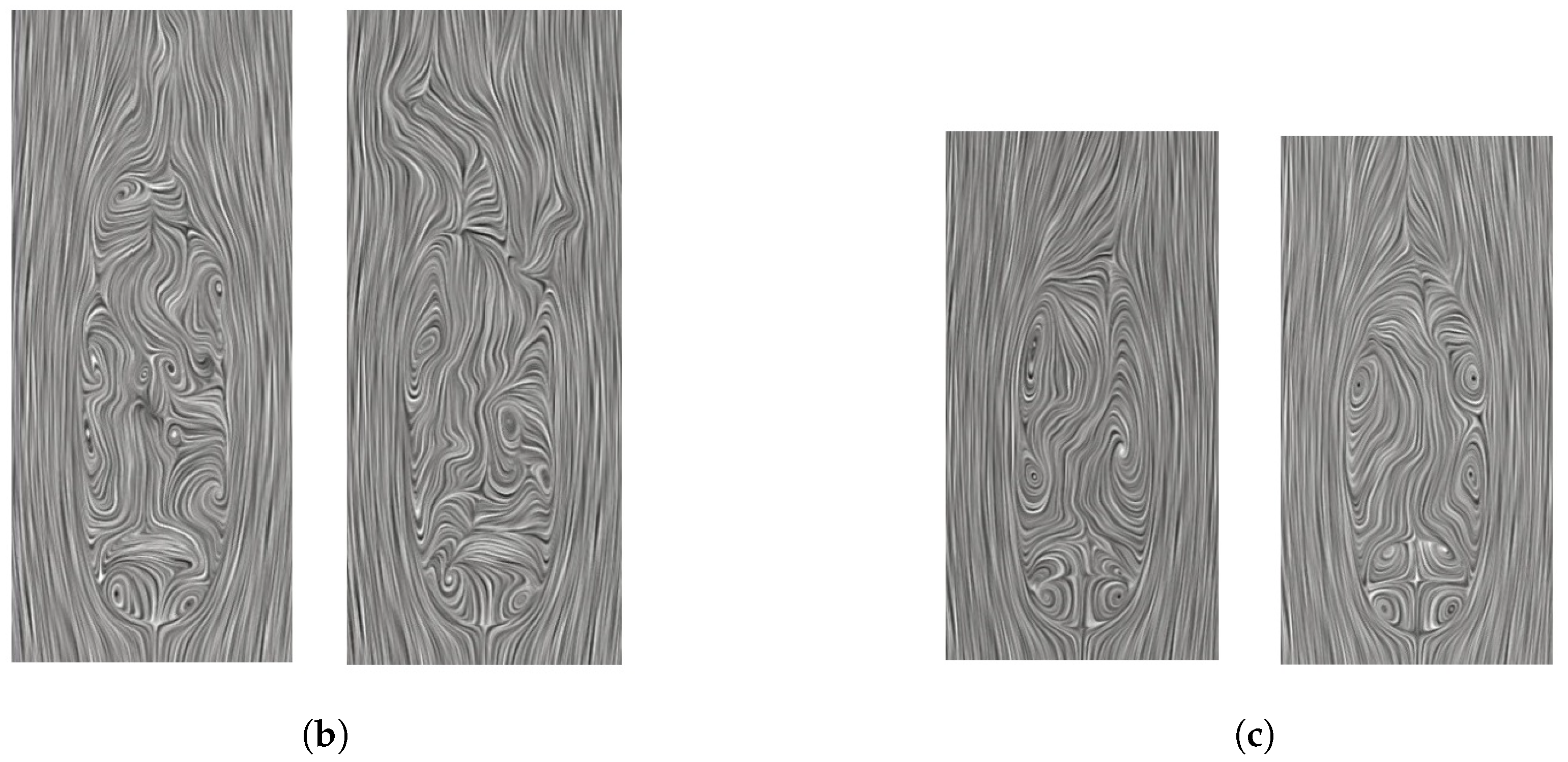
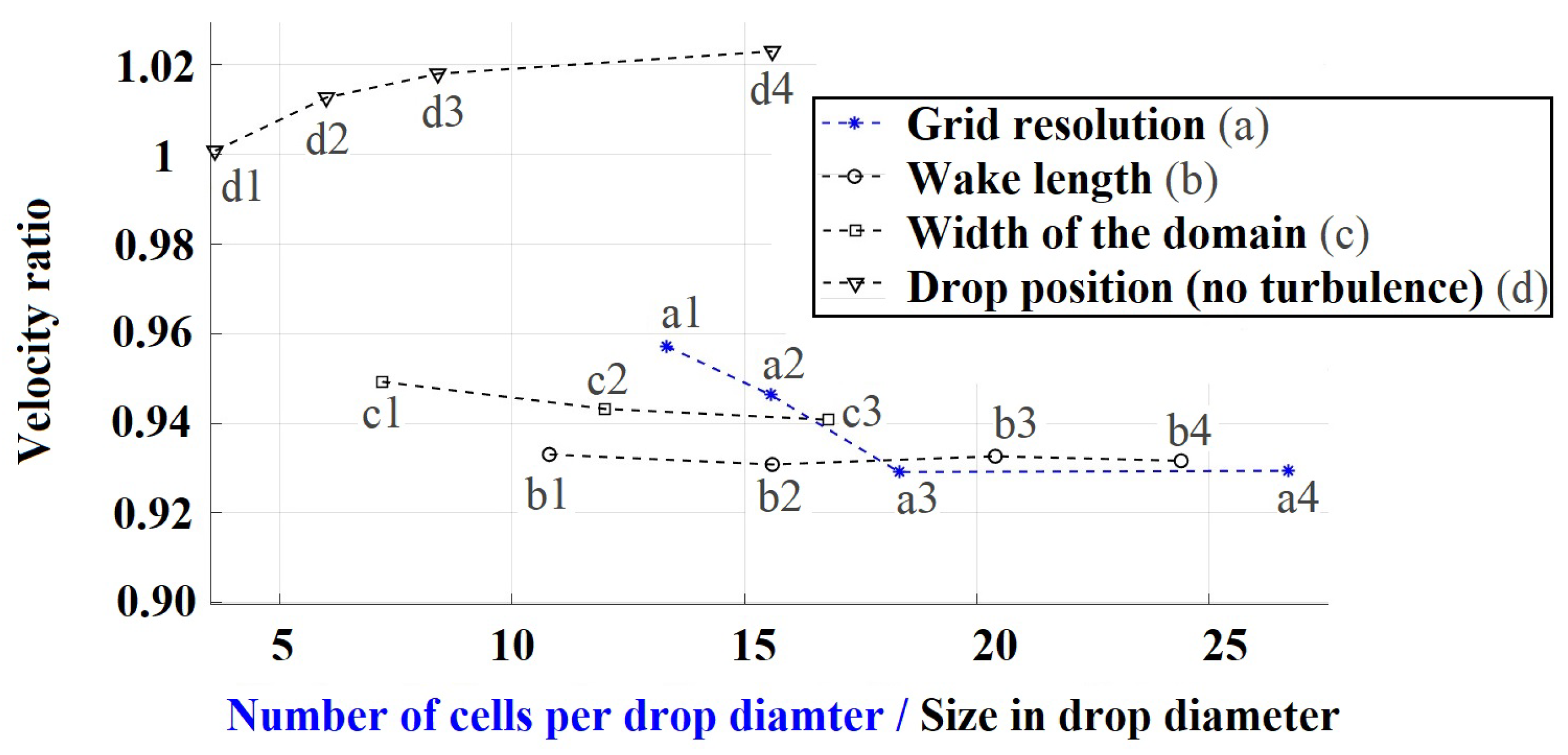
Appendix A. Studies for Grid Resolution and Domain Size

We studied the influence of the grid resolution and domain size (e.g., domain width, drop position, wake length) on the fall velocity of a 3 mm water drop. Except for the study of the drop position, the drop was set to fall in turbulent surroundings with T u = 10%, L t = D/2 at the inflow region. The inertial mean flow velocity of the coming air lies at 7.8 m/s. The strength of turbulent air flow in the stream-wise direction changes due to turbulence decay and should exert a different impact for drop at a different position. Thus, we conducted the study for the drop position with an air flow without turbulence. Simulations for each separate test series were carried out with a time duration that was long enough to quantify the influence of turbulence with different setups. Table A1 presents for each test series the setups for the grid resolution and domain size.
Table A1. Setup for the studies of the grid resolution, the size of the simulation domain and the position of water drop in the main flow direction.
Test SeriesGrid-Cells in a Drop DiameterDomain WidthWake LengthDrop PositionCase Number
Grid Resolution13.37.2D10.8D3.6Da1
15.6 a2
18.3 a3
26.7 a4
Wake Length26.77.2D10.8D3.6Db1
15.6D b2
20.4D b3
24.4D b4
Domain Width26.77.2D18D6.0Dc1
12.0D c2
16.8D c3
Drop Centre in the Stream-wise Direction26.712D15.6D3.6Dd1
6.0Dd2
8.4Dd3
10.8Dd4
Figure A1 summaries the results, the velocity ratios between the simulated fall velocities and v t measured in still air of all cases, from these four studies. Based on the convergence of these results, we chose a grid resolution of 26.7 cells per drop diameter for the further simulations. With this resolution, we resolved the flow field until the Kolmogorov length scale (see Section 3).
Figure A1. Studies of the grid resolution, the domain width and wake length, as well as the position of water drop in the stream-wise direction.
Fluids 05 00158 g0a1
The wake length and domain width were selected as 13.2D and 12D, respectively. We suggest that the deviations of the velocity ratio in the cases d1–d4 are more related to the spacing for the pressure field around the flow stagnation point. A large spacing should provide a more reasonable solution of the flow field. Thus, we selected the position of the drop at a stream-wise direction of 6D, with consideration of the decay in the turbulent air flow from the inlet.

Appendix B. Validations for the Drop Deformation

Figure A2 shows a comparison of the simulated axis ratios, axis ratio amplitudes and drop oscillation frequencies for the 3 mm and 2 mm water drops in still air with results from previous studies. Values from the simulations were averaged over at least 0.5 s after the fall velocity of the water drop stabilised. The axis ratio amplitude was calculated with the difference between the maximum and the minimum temporal axis ratio during the drop oscillation periods. As shown in the figure, the simulated axis ratios and oscillation frequencies of both drops fit quite well with the results from previous studies. The axis ratio amplitudes of both water drops lie near most of the data from previous measurements.
Figure A2. Comparison of the axis ratios, the axis ratio amplitudes and the oscillation frequencies of the simulated 3 mm and 2 mm water drops in stagnant air: (a) Axis ratio. (b) Axis ratio amplitude. (c) Oscillation frequency. The figure is adapted from [30].
Fluids 05 00158 g0a2

References

  1. Hosking, J.; Stow, C. Ground-based measurements of raindrop fallspeeds. J. Atmos. Ocean. Technol. 1991, 8, 137–147. [Google Scholar] [CrossRef]
  2. Sekhon, R.; Srivastava, R. Doppler radar observations of drop-size distributions in a thunderstorm. J. Atmos. Sci. 1971, 28, 983–994. [Google Scholar] [CrossRef] [Green Version]
  3. Pei, B.; Testik, F.; Gebremichael, M. Impacts of raindrop fall velocity and axis ratio errors on dual-polarization radar rainfall estimation. J. Hydrometeorol. 2014, 15, 1849–1861. [Google Scholar] [CrossRef]
  4. Joss, J.; Waldvogel, A. Ein spektrograph für niederschlagstropfen mit automatischer auswertung. Pure Appl. Geophys. 1967, 68, 240–246. [Google Scholar] [CrossRef]
  5. Marshall, J.; Langille, R.; Palmer, W.M.K. Measurement of rainfall by radar. J. Meteorol. 1947, 4, 186–192. [Google Scholar] [CrossRef]
  6. List, R.; Donaldson, N.; Stewart, R. Temporal evolution of drop spectra to collisional equilibrium in steady and pulsating rain. J. Atmos. Sci. 1987, 44, 362–372. [Google Scholar] [CrossRef] [Green Version]
  7. Fornis, R.; Vermeulen, H.; Nieuwenhuis, J. Kinetic energy–rainfall intensity relationship for Central Cebu, Philippines for soil erosion studies. J. Hydrol. 2005, 300, 20–32. [Google Scholar] [CrossRef]
  8. Rosewell, C. Rainfall kinetic energy in eastern Australia. J. Clim. Appl. Meteorol. 1986, 25, 1695–1701. [Google Scholar] [CrossRef] [Green Version]
  9. Fox, N. The representation of rainfall drop-size distribution and kinetic energy. Hydrol. Earth Syst. Sci. Discuss. 2004, 8, 1001–1007. [Google Scholar] [CrossRef] [Green Version]
  10. Panagopoulos, A.; Kanellopoulos, J. Prediction of triple-orbital diversity performance in Earth-space communication. Int. J. Satell. Commun. 2002, 20, 187–200. [Google Scholar] [CrossRef]
  11. Gunn, R.; Kinzer, G. The terminal velocity of fall for water droplets in stagnant air. J. Meteorol. 1949, 6, 243–248. [Google Scholar] [CrossRef] [Green Version]
  12. Löffler-Mang, M.; Joss, J. An optical disdrometer for measuring size and velocity of hydrometeors. J. Atmos. Ocean. Technol. 2000, 17, 130–139. [Google Scholar] [CrossRef]
  13. Testik, F.; Barros, A.; Bliven, L. Field observations of multimode raindrop oscillations by high-speed imaging. J. Atmos. Sci. 2006, 63, 2663–2668. [Google Scholar] [CrossRef]
  14. Montero-Martínez, G.; Kostinski, A.; Shaw, R.; García-García, F. Do all raindrops fall at terminal speed? Geophys. Res. Lett. 2009, 36. [Google Scholar] [CrossRef] [Green Version]
  15. Larsen, M.; Kostinski, A.; Jameson, A. Further evidence for superterminal raindrops. Geophys. Res. Lett. 2014, 41, 6914–6918. [Google Scholar] [CrossRef] [Green Version]
  16. Montero-Martínez, G.; García-García, F. On the behaviour of raindrop fall speed due to wind. Q. J. R. Meteorol. Soc. 2016, 142, 2013–2020. [Google Scholar] [CrossRef]
  17. Niu, S.; Jia, X.; Sang, J.; Liu, X.; Lu, C.; Liu, Y. Distributions of raindrop sizes and fall velocities in a semiarid plateau climate: Convective versus stratiform rains. J. Appl. Meteorol. Climatol. 2010, 49, 632–645. [Google Scholar] [CrossRef]
  18. Thurai, M.; Bringi, V.; Petersen, W.; Gatlin, P. Drop shapes and fall speeds in rain: Two contrasting examples. J. Appl. Meteorol. Climatol. 2013, 52, 2567–2581. [Google Scholar] [CrossRef]
  19. Bringi, V.; Thurai, M.; Baumgardner, D. Raindrop fall velocities from an optical array probe and 2-D video disdrometer. Atmos. Meas. Technol. 2018, 11, 1377–1384. [Google Scholar] [CrossRef] [Green Version]
  20. Stout, J.; Arya, S.; Genikhovich, E. The effect of nonlinear drag on the motion and settling velocity of heavy particles. J. Atmos. Sci. 1995, 52, 3836–3848. [Google Scholar] [CrossRef]
  21. Smith, F. Conditioned particle motion in a homogeneous turbulent field. Atmos. Environ. (1967) 1968, 2, 491–508. [Google Scholar] [CrossRef]
  22. Clift, R.; Grace, J.; Weber, M. Bubbles, Drops, and Particles; Courier Corporation: Chelmsford, MA, USA, 2005. [Google Scholar]
  23. Johnson, T.; Patel, V. Flow past a sphere up to a Reynolds number of 300. J. Fluid Mech. 1999, 378, 19–70. [Google Scholar] [CrossRef]
  24. Sakamoto, H.; Haniu, H. A study on vortex shedding from spheres in a uniform flow. J. Fluids Eng. 1990, 112, 386–392. [Google Scholar] [CrossRef]
  25. Leweke, T.; Provansal, M.; Ormieres, D.; Lebescond, R. Vortex dynamics in the wake of a sphere. Phys. Fluids 1999, 11, S12. [Google Scholar] [CrossRef]
  26. Mittal, R. Planar symmetry in the unsteady wake of a sphere. AIAA J. 1999, 37, 388–390. [Google Scholar] [CrossRef]
  27. Kim, H.; Durbin, P. Observations of the frequencies in a sphere wake and of drag increase by acoustic excitation. Phys. Fluids 1988, 31, 3260–3265. [Google Scholar] [CrossRef]
  28. Yun, G.; Kim, D.; Choi, H. Vortical structures behind a sphere at subcritical Reynolds numbers. Phys. Fluids 2006, 18, 015102. [Google Scholar] [CrossRef]
  29. Van Dyke, M. An Album of Fluid Motion; Parabolic Press: Stanford, CA, USA, 1982. [Google Scholar]
  30. Szakáll, M.; Mitra, S.; Diehl, K.; Borrmann, S. Shapes and oscillations of falling raindrops—A review. Atmos. Res. 2010, 97, 416–425. [Google Scholar] [CrossRef]
  31. Beard, K. Terminal velocity and shape of cloud and precipitation drops aloft. J. Atmos. Sci. 1976, 33, 851–864. [Google Scholar] [CrossRef] [Green Version]
  32. Pruppacher, H.; Klett, J. Microphysics of Clouds and Precipitation, 2nd ed.; Kulwer Academic: Dordrecht, The Netherlands, 1997. [Google Scholar]
  33. Tokay, A.; Beard, K. A field study of raindrop oscillations. Part I: Observation of size spectra and evaluation of oscillation causes. J. Appl. Meteorol. 1996, 35, 1671–1687. [Google Scholar] [CrossRef]
  34. Pruppacher, H.; Beard, K. A wind tunnel investigation of the internal circulation and shape of water drops falling at terminal velocity in air. Q. J. R. Meteorol. Soc. 1970, 96, 247–256. [Google Scholar] [CrossRef]
  35. LeClair, B.; Hamielec, A.; Pruppacher, H.; Hall, W. A theoretical and experimental study of the internal circulation in water drops falling at terminal velocity in air. J. Atmos. Sci. 1972, 29, 728–740. [Google Scholar] [CrossRef] [Green Version]
  36. Szakáll, M.; Diehl, K.; Mitra, S.; Borrmann, S. A wind tunnel study on the shape, oscillation, and internal circulation of large raindrops with sizes between 2.5 and 7.5 mm. J. Atmos. Sci. 2009, 66, 755–765. [Google Scholar] [CrossRef]
  37. Eisenschmidt, K.; Ertl, M.; Gomaa, H.; Kieffer-Roth, C.; Meister, C.; Rauschenberger, P.; Reitzle, M.; Schlottke, K.; Weigand, B. Direct numerical simulations for multiphase flows: An overview of the multiphase code FS3D. Appl. Mathe. Comput. 2016, 272, 508–517. [Google Scholar] [CrossRef]
  38. Hirt, C.; Nichols, B. Volume of fluid (VOF) method for the dynamics of free boundaries. J. Comput. Phys. 1981, 39, 201–225. [Google Scholar] [CrossRef]
  39. Rider, W.J.; Kothe, D.B. Reconstructing volume tracking. J. Comput. Phys. 1998, 141, 112–152. [Google Scholar] [CrossRef] [Green Version]
  40. Popinet, S. An accurate adaptive solver for surface-tension-driven interfacial flows. J. Comput. Phys. 2009, 228, 5838–5866. [Google Scholar] [CrossRef] [Green Version]
  41. Rieber, M. Numerische Modellierung der Dynamik freier Grenzflächen in Zweiphasenströmungen. Ph.D. Thesis, University of Stuttgart, Stuttgart, Germany, 2004. [Google Scholar] [CrossRef] [Green Version]
  42. Harlow, F.; Welch, J. Numerical calculation of time-dependent viscous incompressible flow of fluid with free surface. Phys. Fluids 1965, 8, 2182–2189. [Google Scholar] [CrossRef]
  43. Kornev, N.; Hassel, E. Synthesis of homogeneous anisotropic divergence-free turbulent fields with prescribed second-order statistics by vortex dipoles. Phys. Fluids 2007, 19, 068101. [Google Scholar] [CrossRef]
  44. Zhu, C.; Ertl, M.; Weigand, B. Numerical investigation on the primary breakup of an inelastic non-Newtonian liquid jet with inflow turbulence. Phys. Fluids 2013, 25, 083102. [Google Scholar] [CrossRef]
  45. Baggio, M.; Weigand, B. Numerical simulation of a drop impact on a superhydrophobic surface with a wire. Phys. Fluids 2019, 31, 112107. [Google Scholar] [CrossRef]
  46. Tomboulides, A.; Orszag, S. Numerical investigation of transitional and weak turbulent flow past a sphere. J. Fluid Mech. 2000, 416, 45–73. [Google Scholar] [CrossRef]
  47. Wu, J.; Faeth, G. Sphere wakes in still surroundings at intermediate Reynolds numbers. AIAA J. 1993, 31, 1448–1455. [Google Scholar] [CrossRef]
  48. Rodriguez, I.; Borrell, R.; Lehmkuhl, O.; Segarra, C.; Oliva, A. Direct numerical simulation of the flow over a sphere at Re = 3700. J. Fluid Mech. 2011, 679, 263–287. [Google Scholar] [CrossRef]
  49. Magarvey, R.; Bishop, R. Wakes in liquid-liquid systems. Phys. Fluids 1961, 4, 800–805. [Google Scholar] [CrossRef]
  50. Poon, E.; Iaccarino, G.; Ooi, A.S.; Giacobello, M. Numerical studies of high Reynolds number flow past a stationary and rotating sphere. In Proceedings of the 7th International Conference on CFD in the Minerals and Process Industries, Melbourne, Australia, 9–11 December 2009. [Google Scholar]
Figure 1. Drag coefficients of water drops in stagnant air falling at their terminal velocities (blue dots) (data taken from Gunn and Kinzer [11]) in comparison to the drag curve of rigid spheres suggested by Clift [22].
Fluids 05 00158 g001
Figure 2. Terminal velocities and the corresponding Reynolds numbers for water drops of various diameters in stagnant air; data taken from Gunn and Kinzer [11].
Fluids 05 00158 g002
Figure 3. Computational domain for the fall of a water drop in air flow, displayed in a 2D slice.
Fluids 05 00158 g003
Figure 4. The black curve illustrates the time evolution of the simulated fall velocity of a 3 mm water drop in stagnant air. The dashed line displays the corresponding terminal velocity according to Gunn and Kinzer [11] ( v t = 8.06 m/s).
Fluids 05 00158 g004
Figure 5. Simulated fall velocities of the 3 mm and 2 mm water drops over time: (a) D = 3 mm. (b) D = 2 mm. In the 3 mm drop case D3T0, the curve is obtained from the validation case. For all other cases, the initial mean velocity of the incoming air flow was set to 7.8 m/s and 6.2 m/s for the 3 mm and 2 mm drops, respectively.
Fluids 05 00158 g005
Figure 6. Temporal variations in the axis lengths and surface area of the simulated 3 mm water drop in stagnant air.
Fluids 05 00158 g006
Figure 7. An example for the shape change of the simulated 3 mm water drop, falling in stagnant air.
Fluids 05 00158 g007
Figure 8. Comparison of the instantaneous (stream-wise) velocity field of a 3 mm water drop falling in still air (left) and that falling in turbulent air flow (right).
Fluids 05 00158 g008
Figure 9. Instantaneous streamlines coloured with the normalised stream-wise velocity (left), the vorticity magnitude (middle) and the normalised pressure (right) for the case D3T0, at about 2.3 s.
Fluids 05 00158 g009
Figure 10. Instantaneous streamlines coloured with the normalised stream-wise velocity (left), the vorticity magnitude (middle) and the normalised pressure (right) for the case D3L050T10, at about 1.6 s.
Fluids 05 00158 g010
Figure 11. An example of time-averaged flow over a droplet, showing the position for the base pressure coefficient − C ¯ pb and wake recirculation bubble.
Fluids 05 00158 g011
Figure 12. Comparison of the time-averaged stream-wise velocity along the wake symmetry axis for the simulated sphere with Re = 1000 (dashed line), the 3 mm water drop in still air with Re = 916 (dashed line) and the previous studies. The figure is adapted from [46].
Fluids 05 00158 g012
Figure 13. Comparisons of the Strouhal numbers for the simulated 3 mm and 2 mm water drops in stagnant air, the simulated sphere at Re = 1000 and the spheres from the previous studies. The figure is reproduced from [28] and modified with our simulation results, with the permission of AIP Publishing.
Fluids 05 00158 g013
Figure 14. Simulated base suction pressure coefficient − C ¯ pb with respect to the length of the recirculation region L ¯ / D , as well as the minimum axis pressure coefficient − C ¯ pmin with respect to the wake formation length L ¯ v / D (exact values and the corresponding cases are shown in Table 5).
Fluids 05 00158 g014
Figure 15. Drag coefficients of the simulated water droplets with respect to the lengths of their wake recirculation areas (exact values and the corresponding cases are shown in Table 5).
Fluids 05 00158 g015
Figure 16. Strouhal numbers of the simulated water drops with respect to their drag coefficients (exact values and the corresponding cases are shown in Table 5).
Fluids 05 00158 g016
Figure 17. Reynolds stress component u v ¯ / u 2 for flow past the simulated sphere at Re = 1000.
Fluids 05 00158 g017
Figure 18. Comparison of the Reynolds stresses and turbulent kinetic energy of the 3 mm water drops falling in stagnant and turbulent surroundings: (a) u u ¯ / u 2 . (b) v v ¯ / u 2 . (c) u v ¯ / u 2 . (d) Turbulent kinetic energy. From left to right: cases D3T0, D3L050T10, D3L025T10, D3L050T05, D3L025T05.
Fluids 05 00158 g018
Figure 19. Comparison of the Reynolds stresses and turbulent kinetic energy of the 2 mm water drops falling in stagnant and turbulent surroundings: (a) u u ¯ / u 2 . (b) v v ¯ / u 2 . (c) u v ¯ / u 2 . (d) Turbulent kinetic energy. From left to right: cases D2T0, D2L050T10, D2L025T10, D2L050T05, D2L025T05.
Fluids 05 00158 g019
Figure 20. Streamlines of the 3 mm (Re = 1614) and 2 mm (Re = 916) water drops falling in stagnant air at their terminal velocities: (a) Time-averaged streamlines of the 3 mm (left) and 2 mm (right) water drop. (b) Streamlines of the 3 mm water drop at two different time steps. (c) Streamlines of the 2 mm water drop at two different time steps.
Fluids 05 00158 g020aFluids 05 00158 g020b
Table 1. Physical properties of the air and water drop (20 C) within the simulations.
Air Density
ρ gas (kg/m 3 )
Water Density
ρ l (kg/m 3 )
Air Viscosity
μ gas (Pa · s)
Water Viscosity
μ l (Pa · s)
Surface Tension
σ (N/m)
1.2045998.218.2 × 10 6 1 × 10 3 72.75 × 10 3
Table 2. Terminal velocities, corresponding Reynolds numbers and drag coefficients for 3 mm and 2 mm water drops falling in stagnant air, according to Gunn and Kinzer [11].
Equivalent Drop Diameter (mm)Terminal Velocity (m/s)Reynolds NumberDrag Coefficient
3.08.0616130.503
2.06.498660.517
Table 3. Comparison of the terminal velocities and drag coefficients for the 3 mm and 2 mm water drops in turbulent and stagnant air flows.
Test CasesTerminal Velocity (m/s)Drag CoefficientVelocity DecreaseReynolds NumberWeber Number
D3T08.130.492-16143.28
D3L050T107.550.5707.1%--
D3L025T107.730.5444.9%--
D3L050T057.690.5505.4%--
D3L025T057.830.5303.7%--
D2T06.920.453-9161.59
D2L050T106.640.4924.0%--
D2L025T106.770.4732.2%--
D2L050T056.730.4792.7%--
D2L025T056.850.4621.0%--
Table 4. Comparison of the time-averaged drop axis ratios, horizontal axis lengths, axis ratio amplitudes and oscillation frequencies of the simulated falling water drops in both stagnant and turbulent surroundings.
Test CasesAxis RatioAxis Length 2 a ¯ (mm)Axis Ratio AmplitudeOscillation Frequency
D3T00.8813.1190.08659
D3L050T100.8873.1140.14466
D3L025T100.8863.1150.09162
D3L050T050.8873.1140.08860
D3L025T050.8843.1170.10761
D2T00.9422.0400.064116
D2L050T100.9422.0380.098120
D2L025T100.9422.0380.067116
D2L050T050.9422.0400.083116
D2L025T050.9422.0390.075117
Table 5. Comparison of statistical flow parameters for the simulated water drops falling in stagnant air and turbulent surroundings, e.g., the flow separation angle, base suction pressure, length of the wake recirculation, minimum pressure coefficient, vortex formation length and Strouhal numbers.
θ ¯ s ( ) C ¯ pb L ¯ / D C ¯ pmin L ¯ v / D S t
D3T088.20.2432.820.3131.7870.263
D3L050T1093.60.3411.230.4480.4000.532
D3L025T1092.30.3201.560.4240.6250.430
D3L050T0595.10.3381.470.4380.5880.451
D3L025T0588.70.3061.780.4070.8130.413
D2T090.60.2362.500.3031.4500.167
D2L050T1096.00.2971.360.3880.4750.393
D2L025T1092.20.2701.790.3540.7750.314
D2L050T0593.70.2821.710.3710.7380.313
D2L025T0590.80.2582.090.3341.0000.257

