Abstract
We examine two dimensional properties of vortex shedding past elliptical cylinders through numerical simulations. Specifically, we investigate the vortex formation length in the Reynolds number regime 10 to 100 for elliptical bodies of aspect ratio in the range 0.4 to 1.4. Our computations reveal that in the steady flow regime, the change in the vortex length follows a linear profile with respect to the Reynolds number, while in the unsteady regime, the time averaged vortex length decreases in an exponential manner with increasing Reynolds number. The transition in profile is used to identify the critical Reynolds number which marks the bifurcation of the Karman vortex from steady symmetric to the unsteady, asymmetric configuration. Additionally, relationships between the vortex length and aspect ratio are also explored. The work presented here is an example of a module that can be used in a project based learning course on computational fluid dynamics.
1. Introduction
Vortex development in a fluid’s flow is a highly nonlinear phenomenon which goes through multiple bifurcations. This topic is rarely introduced in a serious manner in an undergraduate course on fluids. However, there are simple ways to talk about vortex development by combining qualitative and quantitative approaches that go beyond simply examining classical images or the use of sophisticated particle image velocimetry (PIV) techniques. We introduce one such method of talking about the physics of vortex development in this paper, which can be used in the form of a lesson plan for a lecture or to motivate computational projects in more advanced classes in fluids. Student-centered practices such as problem-based and project-based learning (PBL) are more commonly practiced in the arts. Instructional methods related to PBL promote a more inductive approach to learning whereby generalizations and abstractions follow from first understanding specific cases [1]. This approach is in contrast to the deductive strategy taken in the sciences which is a more top-down approach and a possible cause of alienation in several students. The concept of problem-based learning began more than 30 years ago in the context of medical education. PBL has been defined as the “posing of a complex problem to students to initiate the learning process” [2] and as “experiential learning organized around the investigation and resolution of messy, real-world problems” [3]. PBL can be implemented at various scales in a course with a focus from a “teacher to student-centered education with process-oriented methods of learning” [4,5]. The recent popularity of project based learning approach in physics and engineering education is based on research indicating the effectiveness of PBL in enhancing student engagement [4,6,7]. Several recent educational papers have specifically discussed the effectiveness of computational problems in fluid dynamics and the use of software such as Comsol, among others, in improving classroom engagement [8,9,10,11,12,13]. The current paper is an attempt to present a similar example of a complex problem in fluid dynamics which is apt as a unit which can be introduced as a project.
Flow past a circular cylinder is a very well studied problem in classical fluid mechanics. While the creeping flow regime is completely understood and most related problems are approachable analytically, the inertial regime contains several unanswered questions. The evolution of flow past a cylinder is a particularly interesting and well studied problem [14]. The Reynolds number (, where U and L represent the characteristic velocity and length respectivel, and refers to the dynamic viscosity) has been shown to capture several critical changes in flow structure. The first of these happens around [15], where the flow transitions from the creeping flow to one with a symmetric vortex profile. A second flow bifurcation from the steady symmetric profile to a asymmetric unsteady vortex occurs at around [16] which lasts until about . Following the notation employed in the recent literature [17], we identify these critical Reynolds numbers as and , respectively. We refer the readers to the paper by Faruquee et al. [17] who provide a thorough discussion of the various historical experimental and numerical studies on this topic. The critical values referred to above are sensitive to shape of the obstacle, aspect ratio (), blockage ratio of channel diameter to channel width, roughness of the cylinder etc. but the qualitative aspects of the various transitions are still maintained.
In this paper we are concerned with highlighting the dynamics of vortex formation, specifically through an examination of the vortex length in a flow past an elliptical obstacle. Experimental measurements of the length and width of wake vortices past cylinders have been discussed in the literature [14,16,18,19,20,21,22,23,24]. The vortex length, usually denoted , is defined as “the streamwise distance between the confluence point (wake stagnation point) and the rear stagnation point of the cylinder” [17]. It is also, more commonly, defined as the distance between the rear stagnation point and the “point downstream where the velocity fluctuation level has grown to a maximum” [14] (Figure 1 provides a schematic explanation of this metric). Experiments and numerics indicate the relation between and maximum velocity fluctuation and the base pressure (at the rear of the obstacle) to be inversely proportional [23,25,26]. Coutanceau and Bouard [27] put forth the linear equation for , which, in the steady, symmetric vortex regime, related the growth of the near wake vortex as a function of .
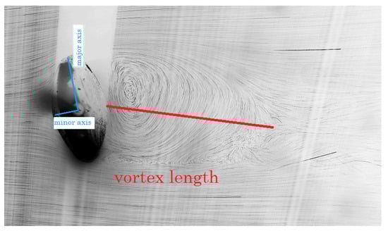
Figure 1.
This figure shows a visualization of the primary vortex region in a flow past an ellipsoidal body. Based on past experimental work [24], the vortex length (denoted by the length of the bold red line) is measured as the distance between the rear surface of the body and the "pinch-off" point where the flow velocity vanishes.
The effect of , which is the ratio of the semi-minor (a) to semi-major (b) axis of the obstacle, is also of interest in this study. Note that indicates an elongated body while, suggests a squat, flat object (such as disk in 3D). In two dimensions the shape itself is identical and therefore the is reflective of the orientation of the body with respect to the oncoming flow. Hence in 2D, we can describe as indicative of a high drag configuration where the entire length of the body is perpendicular to the flow, while in the case of , the body assumes a pefectly streamlined position with the length of the body parallel to the flow. Recent numerical simulations [17] reveal that has a tendency to increase with increasing for . However, for , the wake disappears. For , Faruquee et al. [17] provide the following equation relating the normalized vortex formation length to AR:
where d is the hydraulic diameter. This formula indicates a critical minimum of 0.34 below which no symmetric vortex forms. This critical is sensitive to the and has been shown to increase with decreasing Table 3 [17]. The calculations are in agreement with the experimental studies [27,28].
In the rest of the paper we numerically investigate the vortex formation length for a class of ellipse shaped obstacles in a flow in the range for various s. Our investigation goes past into the asymmetric, periodic vortex shedding regime. Section 2, discusses the numerical method used and Section 3 elaborates the results of our computations and compares them with those in the literature.
Vortex formation in flow past cylinders has been studied extensively for many practical applications. Vortices form when fluids flow past obstacles at sufficiently high speeds and are therefore of particular interest in various branches of engineering as they can pose a threat by inducing harmful vibrations in aircrafts, buildings, and other structures. In the ensuing analysis, we determine the length of the primary vortex region in the wake of an immersed body, since this region is most influential in the dynamics of the body. More specifically, we examine 2D elliptical bodies of different aspect ratio (henceforth denoted ), which is a ratio of semi-major to semi-minor axis (oblate) and semi-minor to semi-major (prolate). A total of thirteen different values of from 0.2 to 2.6, increasing in increments of 0.2, have been considered. This simple numerical approach is a continuation of a previous experiment conducted on a flow past a fixed cylinder in a flow tank, in which the vortex length was determined by means of visualization and serves to elucidate a complex problem by simple means, which we believe makes for an effective class project.
2. Methodology
We used COMSOL Multiphysics to model a 2D flow in a channel past a fixed cylinder. The software uses a finite element method to solve the Navier–Stokes and incompressibility equations given by
Here, is the density of the fluid, u = is the divergence free flow field, t is time, is the kinematic viscosity, and p is the pressure. The Reynolds number is defined as , where U is the far-field of free-stream velocity, ranging between 0.1–1 m/s, d is the characteristic length, which in this case was m and is the dynamic viscosity, taken to be kg/m3. The solution to the above flow equation yielded the velocity and pressure fields which were then utilized to identify the vortex length for and ellipses of varying aspect ratios ( is the ratio of minor axis to major axis). The major and minor axes of the ellipses were chosen to conform to the desired values of but with keeping the area of each ellipse the same as that of the cylinder. Table 1 summarizes the important parameters used in the numerical computations.

Table 1.
The table provides some important parameters for the numerical study. Note that the area of the elliptical cylinders is always maintained at 0.0785 m2 in all calculations.
The problem of flow past a 2D cylinder is a well studied and benchmarked problem in COMSOL [29]. A description of the code and the methodology of this standard problem can also be found on the COMSOL website: comsol.com/model/download/449401/models.mph.cylinder_flow.pdf. For the purposes of this work, this code was suitably adapted for the study of the elliptical cylinder. The problem was solved using the FSI module in COMSOL which uses a PARADISO solver; it was run for 5 s in increments of 0.01 s using a "fine" mesh consisting of 5662 elements. Convergence tests were performed in a previous study [30,31] for a more complex problem involving 2D and 3D elliptical cylinders with attached wings (or flexible fiber).
The dimensions and geometry of the problem studied here were similar to those used in our previous studies [30]. We also verified our code for the case of flow past a circular cylinder with perfect slip conditions along the top and bottom walls and no slip on the surface of the cylinder, to mimic unbounded flow. Through this calculation we were able to obtain the critical bifurcation of around 47 where the flow transitions from steady to unsteady. This helped us to confirm that the metric used to identify the critical Reynolds number was correct. In a classroom setting the relationship between the Reynolds number and the Strouhal number would be appropriate as an additional validation of the numerical scheme. The remaining computations were conducted in a bounded channel with no-slip conditions on the channel walls and also on the surface of the ellipse. The various panels in Figure 2 and Figure 3 show some sample flow and pressure profiles based on our numerical simulations for various Reynolds numbers.
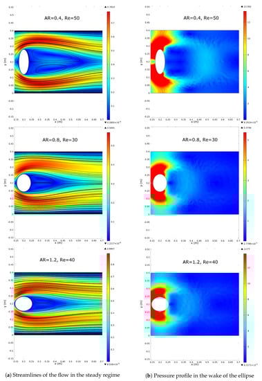
Figure 2.
Numerical simulations of the flow past elliptical objects of various ARs: steady flow.
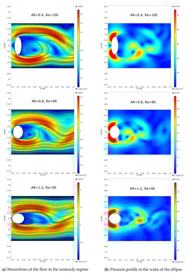
Figure 3.
Numerical simulations of the flow past elliptical objects of various ARs: unsteady flow
Two different criteria were used to measure the length of the vortex depending on whether the flow is steady or unsteady. For the steady case, since the flow does not vary in time (see the top panels in Figure 4), the vortex region is symmetric about and its length remains constant in time. In this case, we examined the horizontal component of the velocity, , and of the pressure gradient, namely, as a function of x along . The border or separatrix of the primary vortex pair separates the inner wake flow from the outer uniform flow. At the junction of the separatrix and , the two flows are in opposing directions, the outer flow moving in the positive x while the wake flow moves in the negative x direction. The point at which can therefore be defined as a critical point which marks the end of the primary vortex region. The horizontal distance of this critical point from the rear end of the cylinder is defined as the vortex length. To confirm this hypothesis, a second criterion was also tested. We also observe that the pressure along increases the fastest as we cross the critical point. Therefore the vortex length can also be defined with respect to the maximum of the magnitude of the pressure gradient. Since is negligible, this collapses to the maximum of along .
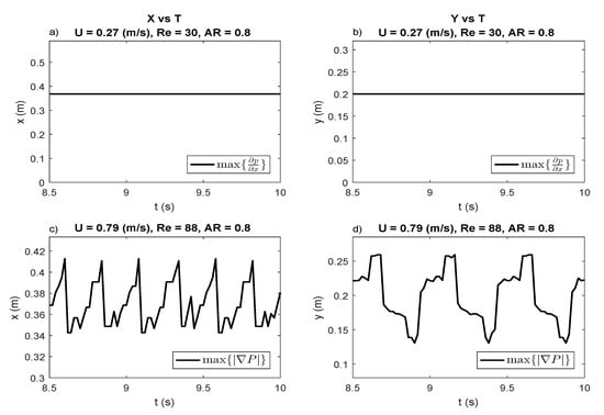
Figure 4.
The panels (a,b) show the position of the wake stagnation point in the case of steady flow, while panels (c,d) show the periodically changing position of the stagnation point for the oscillating flow regime.
In the case when flow becomes unsteady, the wake region oscillates in space and time (see the bottom panels in Figure 4). The vortex region is asymmetric about and moves in both spatial directions x and y. In this case the critical point at a given time was defined by the maximum of the magnitude of the pressure gradient, , which is a generalization of the criterion used in the steady state case and the appropriate length is the time averaged vortex length over a period. We use numerical interpolation to smooth the data and find our zeros and extremum.
3. Results and Discussion
The computations for the steady case show a monotonic increase in vortex length with increasing , below a critical threshold, for all s (see for example, Figure 5). The rising trend is similar for both criteria employed to measure the vortex length. When the flow becomes unsteady, the mean vortex length is seen to decrease with increasing . The maximum vortex length can be associated with the onset of a transition in stability as the flow bifurcates from steady to unsteady Karman vortex. The Figure 5a–d show the mean change in vortex length versus for some sample cases of flow past ellipses of 0.4, 0.8, 1.0, and 1.2. All graphs, show the same overall profile and the turning point can be used to identify the critical Reynolds number, which is sensitive to the of the body. The Table 2 depicts the versus profile for , i.e., for flows that generate a steady vortex, which is in keeping with the linear relationship proposed by Coutanceau and Bouard [27]. The table shows the slopes of best fit lines for various s which appear to monotonically decrease with increasing and are overall close to the value suggested in the literature. In the regime , we use an exponential decaying function, to fit the data. Table 2 also shows the value of the exponent, , along with the goodness of fit for various AR. As in the case of the steady vortex, the dependence of the vortex formation length on is sensitive to AR. The missing data for is due to the termination of our study at ; at this point the case does not reveal an unsteady vortex. Table 3 also shows the average for different and .
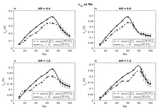
Figure 5.
The figures show the change in normalized vortex length, , versus for in (a), in (b), in (c) and in (d). The maximum point in each graph characterizes the transition at which the flow changes from steady symmetric to unsteady asymmetric.
Table 2.
This table shows the nature of the vs. relationship in the two different flow regimes. The first two rows provide the slope of the best line representing the changing value of in the steady wake. Rows three and four tabulate the exponentially decaying rate of as a function of in the unsteady, asymmetric wake.
Table 3.
The table shows the average values of the normalized vortex length for various values of and .
A particularly interesting relationship to investigate in this problem is that between the critical Reynolds numbers, and . The transitions from steady to unsteady wake are very sensitive to the specific geometric characteristics of the cylinder. Figure 6 shows the critical for s ranging between 0.4 and 1.4 estimated from using the velocity and pressure gradient criteria. The vs. curve shows a minimum at 0.6–0.7. Overall, for bodies with in the range 0.4–1.4, appears to lie in the range 55–95; for a cylinder our calculations show this critical value to lie at the accepted value of . The more streamlined bodies show greater propensity to develop elongated primary vortices. The equation:
captures the quadratic nature of the profile (with value of 0.96) seen in Figure 6, obtained by fitting the average of the two curves shown in the figure. This equation gives us valuable information about the optimal geometry and its relationship with vortex formation. Engineers and designers wanting to suppress disruptive osculations may find this equation particularly useful.
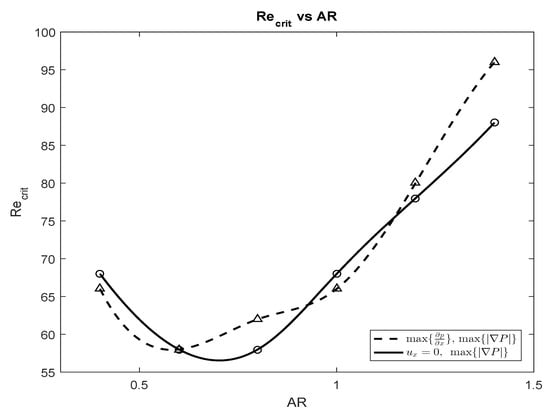
Figure 6.
The graph shows the variation of versus .
4. Conclusions
In summary, our overall computations and qualitative profiles are in agreement with previous experimental results [24], where measurements of variations in vortex length were made through flow visualization and imaging techniques of flow past various cylinders in a flow tank. These experiments indicate a similar extremum in vortex length as a function of flow speed () and . The central contribution of this work lies in two consistent ways of defining the vortex formation length and the observation of the vortex length dependence on , especially in the unsteady flow regime. Questions for future investigation include extending the regime of the study and experimental verification of the unsteady vortex formation length. Pedagogical treatments in the literature appear to focus primarily on lower level courses in science and engineering. There is little discussion about the teaching and learning of more advanced topics like fluid dynamics [32]. We believe that examples like the ones presented here add value to the science of fluid dynamics in some capacity, but also to the ways in which students can engage with difficult topics in fluid dynamics. Such a treatment lends itself very well to a first serious course in fluids but also in more advanced courses where students have greater proficiency in dealing with computational software like Comsol.
Author Contributions
The computations in this paper were performed while M.K. was a graduate student at Montclair State University. Authors B.G.N. and A.V. designed the study, helped analyze the results and wrote the paper. All authors have read and agreed to the published version of the manuscript.
Funding
This research received no external funding.
Conflicts of Interest
The authors declare no conflict of interest.
References
- Connor, J. Project Based Learning and Authenticity: An Instructor’s View. In Proceedings of the 7th First Year Engineering, Roanoke, VA, USA, 3–4 August 2015. [Google Scholar]
- Sahin, M.; Yorek, N. A comparison of problem-based learning and traditional lecture students expectations and course grades in an introductory physics classroom. Sci. Res. Essays 2009, 4, 753–762. [Google Scholar]
- Torp, L.; Sage, S. Problem as Possibilities, Problem Based Learning for K-16; Association for Supervision and Curriculum Development: Alexandria, VA, USA, 2002. [Google Scholar]
- Ahlfeldt, S.; Mehta, S.; Sellnow, T. Measurement and analysis of student engagement in university classes where varying levels of PBL methods of instruction are in use. High. Educ. Res. Dev. 2005, 24, 5–20. [Google Scholar] [CrossRef]
- Dahlgren, M.A. Portraits of PBL: Course objectives and students’ study strategies in computer engineering, psychology and physiotherapy. Instr. Sci. 2000, 28, 309–329. [Google Scholar] [CrossRef]
- Hake, R.R. Interactive-engagement versus traditional methods: A six-thousand-student survey of mechanics test data for introductory physics courses. Am. J. Phys. 1998, 66, 64–74. [Google Scholar] [CrossRef]
- Zyngier, D. Listening to teachers—Listening to students: Substantive conversations about resistance, empowerment and engagement. Teach. Teach. Theory Pract. 2007, 13, 327–347. [Google Scholar] [CrossRef]
- Bot, L.; Gossiaux, P.B.; Rauch, C.P.; Tabiou, S. Learning by doing: A teaching method for active learning in scientific graduate education. Eur. J. Eng. Educ. 2005, 30, 105–119. [Google Scholar] [CrossRef]
- Kwon, H.J. Use of comsol simulation for undergraduate fluid dynamics course. ASEE Comput. Educ. (CoED) J. 2013, 4, 63. [Google Scholar]
- Mokhtar, W. Project-Based Learning (PBL): An Effective Tool to Teach an Undergraduate CFD Course. In Proceedings of the 2011 ASEE Annual Conference & Exposition, Vancouver, BC, Canada, 26–29 June 2011. [Google Scholar]
- Mokhtar, W. Using Computational Fluid Dynamics to Introduce Critical Thinking and Creativity in an Undergraduate Engineering Course. Int. J. Learn. 2010, 17, 441–457. [Google Scholar] [CrossRef]
- Pawar, S.; San, O. CFD Julia: A learning module structuring an introductory course on computational fluid dynamics. Fluids 2019, 4, 159. [Google Scholar] [CrossRef]
- Vianna, R.S.; Cunha, A.M.; Azeredo, R.B.; Leiderman, R.; Pereira, A. Computing Effective Permeability of Porous Media with FEM and Micro-CT: An Educational Approach. Fluids 2020, 5, 16. [Google Scholar] [CrossRef]
- Williamson, C.H. Vortex dynamics in the cylinder wake. Annu. Rev. Fluid Mech. 1996, 28, 477–539. [Google Scholar] [CrossRef]
- Marris, A.W. A review on vortex streets, periodic wakes, and induced vibration phenomena. J. Basic Eng. 1964, 86, 185–193. [Google Scholar] [CrossRef]
- Williamson, C.H. Defining a universal and continuous Strouhal Reynolds number relationship for the laminar vortex shedding of a circular cylinder. Phys. Fluids (1958–1988) 1988, 31, 2742–2744. [Google Scholar] [CrossRef]
- Faruquee, Z.; Ting, D.S.; Fartaj, A.; Barron, R.M.; Carriveau, R. The effects of axis ratio on laminar fluid flow around an elliptical cylinder. Int. J. Heat Fluid Flow 2007, 28, 1178–1189. [Google Scholar] [CrossRef]
- Linke, W. New measurements on aerodynamics of cylinders particularly their friction resistance. Phys. Z. 1931, 32, 900. [Google Scholar]
- Rosenhead, L. Vortex systems in wakes. Adv. Appl. Mech. 1953, 3, 185–195. [Google Scholar]
- Berger, E.; Wille, R. Periodic flow phenomena. Annu. Rev. Fluid Mech. 1972, 4, 313–340. [Google Scholar] [CrossRef]
- Morkovin, M.V. Flow around circular cylinder a kaleidoscope of challenging fluid phenomena. In Proceedings of the ASME Symposium on Fully Separated Flows, Philadelphia, PA, USA, 18–20 May 1964; pp. 102–118. [Google Scholar]
- Oertel, H., Jr. Wakes behind blunt bodies. Annu. Rev. Fluid Mech. 1990, 22, 539–562. [Google Scholar] [CrossRef]
- Zdravkovich, M.M. Flow around circular cylinders. Fundamentals 1997, 1, 566–571. [Google Scholar]
- Chung, B.; Cohrs, M.; Ernst, W.; Galdi, G.P.; Vaidya, A. Wake cylinder interactions of a hinged cylinder at low and intermediate Reynolds numbers. Arch. Appl. Mech. 2016, 86, 627–641. [Google Scholar] [CrossRef]
- Roshko, A. On the wake and drag of bluff bodies. J. Aeronaut. Sci. 2012, 22, 124–132. [Google Scholar] [CrossRef]
- Williamson, C.H.K.; Roshko, A. Measurements of base pressure in the wake of a cylinder at low Reynolds numbers. Z. Flugwiss. Weltraumforsch. 1990, 14, 38–46. [Google Scholar]
- Coutanceau, M.; Bouard, R. Experimental determination of the main features of the viscous flow in the wake of a circular cylinder in uniform translation. Part 1. Steady flow. J. Fluid Mech. 1977, 79, 231–256. [Google Scholar] [CrossRef]
- Taneda, S. Experimental investigation of the wakes behind cylinders and plates at low Reynolds numbers. J. Phys. Soc. Jpn. 1956, 11, 302–307. [Google Scholar] [CrossRef]
- Schafer, M.; Turek, S.; Durst, F.; Krause, E.; Rannacher, R. Benchmark computations of laminar flow around a cylinder. In Flow Simulation with High-Performance Computers II; Vieweg+Teubner Verlag: Wiesbaden, Germany, 1996; pp. 547–566. [Google Scholar]
- Allaire, R.; Guerron, P.; Nita, B.; Nolan, P.; Vaidya, A. On the equilibrium configurations of flexible fibers in a flow. Int. J. Non-Linear Mech. 2015, 69, 157–165. [Google Scholar] [CrossRef]
- Nolan, P. Numerical Study of Body Shape and Wing Flexibility in Fluid Structure Interaction. Master’s Thesis, Montclair State University, Montclair, NJ, USA, 2015. [Google Scholar]
- Vaidya, A. Teaching and Learning of Fluid Mechanics. Fluids 2020, 5, 49. [Google Scholar] [CrossRef]


© 2020 by the authors. Licensee MDPI, Basel, Switzerland. This article is an open access article distributed under the terms and conditions of the Creative Commons Attribution (CC BY) license (http://creativecommons.org/licenses/by/4.0/).