Article

Acceleration Waves in Rational Extended Thermodynamics of Rarefied Monatomic Gases

Department of Mathematics and Alma Mater Research Center on Applied Mathematics AM2, University of Bologna, via Saragozza 8, 40123 Bologna, Italy
*
Author to whom correspondence should be addressed.
Fluids 2020, 5(3), 139; https://doi.org/10.3390/fluids5030139
Submission received: 20 July 2020 / Revised: 18 August 2020 / Accepted: 20 August 2020 / Published: 25 August 2020
(This article belongs to the Special Issue Classical and Modern Topics in Fluid Dynamics and Transport Phenomena)

Abstract

:
Rational Extended Thermodynamics theories with different number of moments are usually introduced to study non-equilibrium phenomena in rarefied gases. Here, we use them to describe one-dimensional acceleration waves in a rarefied monatomic gas. In particular, we focus on the degeneracy of the acceleration wave to a shock wave, in order to test the validity of the models and the role played by an increasing number of moments. As a byproduct, some peculiarities of the characteristic velocities at equilibrium are analyzed as well.

1. Introduction

Acceleration waves, also known as weak discontinuity waves, are propagating surfaces across which all the field variables are continuous but some or all the first derivatives of the field variables exhibit a jump [1,2,3]. In particular, this is the case for the velocity that presents a jump of acceleration, hence the name acceleration wave. They can be generated by a small compressive disturbance in a gas that occurs, for example, in a gas flow induced by the motion of a piston advancing with finite acceleration. If the gas behavior is described by a set of hyperbolic conservation laws as those of the Euler model, neglecting the effect of viscosity and conductivity, it is possible to show analytically that the acceleration wave transforms into a shock wave in a finite time, independently from the amplitude of the initial disturbance [3,4,5]. This mathematical prediction does not find evidence in experimental data. In fact, experiments show that such discontinuity does not exist [6]. In this way, acceleration waves can be used as a bench test for a gas theory. In order to have a prediction in accordance with physical observations, it is necessary to describe the gas with a hyperbolic partial differential equation (PDE) system, avoiding the paradox of infinite propagation velocity, typical of parabolic equation systems. However, this is not a sufficient condition: many authors stressed that a suitable dissipation is also required [3,4,7]. Under such conditions, the theory usually predicts the existence of a critical amplitude A c r and a critical time t c r [2,3,5,7,8,9]. If the initial wave amplitude is greater than A c r , the evolution of the weak discontinuity, after the time t c r , brings to the shock formation. In other words, dissipation has a stabilizing effect on the acceleration wave, at least if the initial disturbance is not “too big”. Of course, this effect is much more realistic if it predicts critical amplitude and critical time compatible with physics.
Rational Extended Thermodynamics (RET) is a well-known theory, developed to describe non-equilibrium phenomena in rarefied gases. Its new idea with respect to classical thermodynamics is to consider as independent field variables not only the usual ones (mass density, momentum, energy) but also non-equilibrium quantities like viscous tensor, heat flux, and others. The corresponding equation system is composed by balance laws supplemented by local and instantaneous constitutive equations that satisfy universal physical principles, like the entropy principle and the principle of relativity. Such constitutive relations are determined following different approaches. At a microscopic level, one can refer to the Maximum Entropy Principle (MEP) [10,11,12], following a procedure that starts from the construction of an infinite hierarchy of moments derived from the Boltzmann equation and its subsequent truncation at some order n. The closure of the resulting truncated system is obtained by prescribing the form of the suitable “truncated” distribution function through MEP. A simple example of RET theory is the Grad 13-moment system [13] that was employed to describe various physical phenomena. More in general, the hyperbolic PDE systems of RET, initially proposed by Müller, Ruggeri and other researchers for monatomic gases, were capable of describing phenomena far from equilibrium well, sometimes requiring a high number of moments (like in light scattering phenomena) [10]. Recently, RET has been generalized also to rarefied polyatomic gases providing relevant results and good agreement with experimental data [11,14].
In the present paper, we will consider different RET theories associated with n   =   3 ,   4 ,   ,   7 that consist of 20, 35, 56, 84, and 120 moments, respectively. They form a set of nesting theories such that a model with M moments includes all the field variables of preceding theories with N moments (if M   >   N ). We stress that an increasing truncation order n and, consequently, an increasing number of moments M could be required to describe physical phenomena further from equilibrium or more rarefied gases.
In the past, the behavior of acceleration waves was already studied for the RET 13-moment system by Ruggeri and Seccia, who show that the critical amplitude and decay coefficients of the weak discontinuity waves are big enough to make a physical detection of the phenomena impossible. Starting from these results, here we try to extend the investigation to RET systems with more moments, in order to understand which is the effect of an increasing truncation order (or number of moments) on the acceleration wave behavior. What we discover is in complete agreement with the experiments. In addition, it shows a small effect due to the variation of n that is more evident on the decay behavior of the fastest acceleration wave (which is the wave that propagates with the maximum characteristic speed of the theory). To our knowledge, the complete analysis of the one-dimensional expression of the present RET models in relation to the acceleration waves is available here for the first time. The study shows, as a byproduct, a peculiar property of the characteristic velocities of the different RET theories obtained with different truncation order, which confirms the elegant mathematical properties of RET systems.
The paper is organized as follows: In Section 1, the procedure to construct a RET theory and its properties are briefly summarized, while the theory of the acceleration waves is presented in Section 2. The behaviors of the acceleration waves modeled by RET equations with 20, 35, 56, 84, and 120 moments are presented in Section 3 and analyzed and commented on in Section 4. The Appendix contains some additional relations and calculations.

2. Rational Extended Thermodynamics Models for Monatomic Gases

As mentioned in the Introduction, different approaches could be employed to construct a Rational Extended Thermodynamics theory for a monatomic rarefied gas. In fact, it is possible to write down the field equations at a macroscopic level requiring the validity of universal principles such as the relativity and the entropy principle. Alternatively, the technique introduced by Grad to obtain his famous 13-moment system [13] can be extended to a theory with many moments. Finally, starting from the Boltzmann equation, one can construct an infinite hierarchy of moment equations that is truncated at a certain order and closed through the Maximum Entropy Principle method (MEP) [10,11]. When many moments are taken into account, as in the present work, this last procedure is the easiest to use and implement [10,11,15,16].
It is well-known that at a microscopic level (kinetic theory) the state of a rarefied gas is described by means of the phase density f   ( x ,   c ,   t ) , so that f   ( x ,   c ,   t ) d c represents the number density of the monatomic molecules at point x   =   ( x 1 ,   x 2 ,   x 3 ) and time t with velocities between c and c   +   d c ( c   =   ( c 1 ,   c 2 ,   c 3 ) ). In this framework, the Boltzmann equation describes the time evolution of f:
t f + j = 1 3 c j x j f = Q ,
where Q denotes the collision term, and t · = · / t , x j · = · / x j . If m denotes the mass of the monatomic molecule, the moments are defined as
F = m R 3 f d c , F i 1 i 2 i k = m R 3 c i 1 c i 2 c i k f d c with i k = 1 , 2 , 3 and k = 1 , 2 ,
while the production terms are
P i 1 i 2 i k = m R 3 c i 1 c i 2 c i k Q d c with i k = 1 , 2 , 3 and k = 1 , 2 , ,
and the following infinite moment hierarchy is deduced from (1)
t F + x j F j = 0 F + t F i 1 + x j F j i 1 = 0 F + t F i 1 i 2 + x j F j i 1 i 2 = P i 1 i 2 F + t F i 1 i 2 i 3 + x j F j i 1 i 2 i 3 = P i 1 i 2 i 3 t F i 1 i 2 i k + x j F j i 1 i 2 i k = P i 1 i 2 i k ,
where repeated indexes imply their sum, so for example here j = 1 3 is omitted. We recall that the first five scalar equations correspond to the usual conservation laws of mass, momentum, and energy, and we remark that the set of equations presents a very peculiar structure, since the flux of one equation is equal to the density of the next equation. The infinite PDE system (4) is usually truncated at a certain order n and closed, expressing the last flux and the productions as functions of the densities. As anticipated before, a way to prescribe the a priori unknown constitutive relations between densities, production terms, and last flux is to refer to MEP that fixes the form of the approximated phase density corresponding to the truncated hierarchy
f n = exp ( 1 m χ n / k B ) if χ n = A = 0 n u A c A ,
where k B denotes the Boltzmann constant, while the main field components u A and the quantity c A are [10,11]:
u A = u if A = 0 u i 1 i A if 1 A n , c A = 1 if A = 0 c i 1 c i A if 1 A n .
By construction, the closed truncated system turns out to be globally hyperbolic with a convex extension. The previous relations and the previous results are valid only if integrals (2) are convergent, and this is a delicate question far from equilibrium. In particular, it was proven that in (5) n has to be even [17].
At equilibrium, the phase density reduces to the Maxwellian one ( f M ) and most frequently f n is linearized in the neighborhood of an equilibrium state as
f n ( 1 ) = f M ( 1 m k B ( χ n χ n | E ) ) ,
also taking into account that at equilibrium all the main field components vanish except the first five. The approximation overcomes the convergence problems, so that, for example, a theory associated with an odd truncation order is not allowed far from equilibrium, but its linearization in the neighborhood of an equilibrium state can always be defined. This is the case of the Grad 13-moment system.
Unfortunately, for the linearized RET models expressed in the physical variables, the hyperbolicity property is valid only locally [10,11,16].
In the present paper, we will consider linearized theories obtained through the previous procedure for different values of the truncation order n (see, for example, [10]) that correspond to RET models with different number of moments M (denoted from now on by ET M ). Often, not all the moments associated with the prescribed order n are taken into account; this happens, for example, with the ET 13 that corresponds to n = 3 , but only the trace of the third order tensor F i m m = m = 1 , j = m 3 F i j m is included in the density components (for more details, see [10,11]). However, in the present work, we will focus on the ET M models that consider as independent field variables all the moments of order less or equal to the n. Such systems are also known as n-system and they contain a number of moments, given by [10,11]:
M = ( n + 1 ) ( n + 2 ) ( n + 3 ) 6 .
Denoting with F , F j and P density, flux and production vectors [10,11]:
F ( F , F i 1 , F i 1 i 2 . F i 1 i 2 i N ) T , F j ( F j , F j i 1 , F j i 1 i 2 F j i 1 i 2 i n ) ,
P ( 0 , 0 i 1 , P i 1 i 2 , P i 1 i 2 i n )
(the 0 i 1 denotes the zero vector and the trace of P i 1 i 2 vanishes), the final set of balance laws of ET M can be written in a very concise form:
t F + x i F i = P .
We recall also that, in general densities, fluxes and production terms are determined under the assumption of zero macroscopic gas velocity v obtaining the corresponding non-convective quantities F ˜ i 1 i 2 i k and P ˜ i 1 , i 2 , · , i k . After that, the dependence on the velocity is prescribed by the requirement of Galilean invariance, as shown by Ruggeri in ([18]) where he introduced a general procedure that allows for passing from the convective to the non-convective quantities in a very elegant way. Boillat and Ruggeri [17,19] have also shown that there are strong relations between RET theory with an increasing number of moments, since they constitute nesting theories. In fact, an RET theory with M moments presents characteristic speeds that are contained in the interval between the minimum and the maximum characteristic speed of a theory with N moments, if N > M and ET M is a subsystem of ET N . This will be the case of our n-systems.
In the present paper, we will focus on one-dimensional phenomena that involve one-dimensional field variables. If u is the vector of such variables, system (8) can be written as
C ( u ) t u + D ( u ) x u = P ,
where for simplicity we denote x = x 1 and v = v 1 , while C ( u ) = u F and D ( u ) = u F 1 are square matrices. The system can also be rewritten referring to the material time derivative ˙ = t + v x :
u ˙ + B ( u ) x u = P ( u )
and we will use this last form in the next sections. A final remark concerns a possible simplification of the notation for this peculiar case under investigation. In fact, the one-dimensional ET M system will involve only some of the M-moment components that we can denote by F h , j and define
F h , j = R 3 c 1 h c 2 j f n d c , and F ˜ h , j = R 3 C 1 h C 2 j f n d C ,
where h = 0 , 1 , n and j = 0 , 1 , n / 2 with h + 2 j n ; moreover, F ˜ h , j indicates the non-convective part of F h , j and C i = c i v i the peculiar velocity. The non-equilibrium non-convective part of F h , j will be indicated from now on with
ρ h , j = F ˜ h , j F ˜ h , j | E ,
so that, for example, F ˜ 0 , 0 = ρ , F ˜ 0 , 1 = 3 p , F ˜ 2 , 0 = p + σ , F ˜ 1 , 1 = 2 q and, consequently, ρ 0 , 0 = ρ 0 , 1 = 0 , ρ 2 , 0 = σ , ρ 1 , 1 = 2 q , if ρ is the mass density, p the pressure, σ the 1-component of the viscous tensor, and q the 1-component of the heat flux.

3. Acceleration Waves

An acceleration wave, known also as weak discontinuity, is a propagating surface Γ across which all the field variables are continuous, while the first derivatives of one or more field variables present a jump. Let us suppose that the Cartesian equation of wave front Γ is φ ( x , t ) = 0 and that such surface separates the space into two subspaces: in front, the field variables u 0 ( x , t ) are known and unperturbed, while behind Γ the perturbed field variables u ( x , t ) are in general unknown. If we consider an acceleration wave and denote by [ [ · ] ] = ( . ) φ = 0 ( . ) φ = 0 + the jump across Γ , we have [ [ u ] ] = 0 , while [ [ u φ ] ] = A 0 . Here, we focus on the one-dimensional models and one-dimensional acceleration waves. Under such assumptions, the field equations reduce to (10) if u = u ( x , t ) is the M-dimensional vector of the field variables, B is the corresponding square M × M matrix, and P the M-dimensional vector of the production terms.
Regarding the one-dimensional weak discontinuity waves, it is well known that [1,2,3]
  • The normal velocity V = φ t / | φ | of the wave front coincides with a characteristic speed of system (10) evaluated in the unperturbed field: V = λ ( u 0 ) .
  • The jump vector A is proportional to the right eigenvector r (of matrix B ) corresponding to λ , evaluated in u 0 , so that A = A r ( u 0 ) .
  • The scalar amplitude A satisfies the Bernoulli equation, if d / d t denotes the time derivative along the characteristic line (in our case, d x / d x = λ ( u 0 ) and a ( t ) and b ( t ) are suitable function of the time t):
d A d t + a ( t ) A 2 + b ( t ) A = 0 ,
whose solution can be written as
A ( t ) = A ( 0 ) exp ( 0 t b ( s ) d s ) 1 + A ( 0 ) 0 t a ( s ) e x p ( 0 s b ( χ ) d χ ) d s .
For a one-dimensional space, it was shown that [3]
a ( t ) = φ x u λ · r | 0 , b ( t ) = r T ( u l ) T u l · d u d t + ( u λ · r ) ( l · x u ) u ( l · P ) · r | 0 , d φ x d t + ( u λ · x u ) | 0 φ x = 0 with φ x ( 0 ) = 1 ,
where φ x = φ x and l denote the left eigenvector of B , assuming that l · r = 1 For the sake of completeness, we have also to recall that there are different acceleration waves. If u λ · r = 0 u (hence also a vanishes), the wave is called exceptional, the Bernoulli equation reduces to a linear differential equation whose solution decays in time if b > 0 :
A ( t ) = A ( 0 ) exp ( 0 t b ( s ) d s ) .
In contrast, if u λ · r 0 , for suitable initial values A ( 0 ) ( | A ( 0 ) > | A c r | ), there exists a critical time t c r such that the solution (14) diverges and the acceleration wave degenerates into a shock structure. Accordingly, the field variables are no more continuous across the wave front.
In the cases studied in the next sections, the acceleration waves will propagate in an unperturbed constant equilibrium state u 0 = u E , in which the characteristic speed λ ( u E ) turns out to be constant, so that φ x = 1 t > 0 , and consequently a and b turn out to be constant as well:
a = u λ · r | E and b ( t ) = l · u P r | E ,
so the corresponding formula for A becomes
A ( t ) = A ( 0 ) exp ( b t ) 1 A ( 0 ) a b ( exp ( b t ) 1 ) .
Consequently, the value of the critical time is
t c r = 1 b ln 1 + b a A ( 0 ) ,
if b > 0 (this will be true in all the following examples), t c r is positive if and only if the initial value of the scalar amplitude satisfies the condition A ( 0 ) > b / a for a < 0 , or A ( 0 ) < b / a for a > 0 . The choice of left and right eigenvectors deserves special notice. In principle, they are both defined apart from an arbitrary factor. The arbitrary factor of the left eigenvector can be prescribed by the condition l · r = 1 , while for the right eigenvector the arbitrary factor is somehow absorbed by the scalar amplitude A. However, if the characteristic speed λ | E does not vanish, one can choose the arbitrary factor of r referring to the Hadamard relation, in order to obtain the time evolution equation for the acceleration jump G [11]. In all the RET models analyzed in the next sections, the second component of u corresponds to the velocity of the gas along the x direction, in other words A 2 = A r 2 = [ [ v x ] ] and, thanks to the Hadamard condition, the acceleration gap across the wave front has to satisfy the following relation:
G = v t = λ | E v x = λ | E A r 2 .
Hence, if the second component of the right eigenvector is chosen as r 2 = 1 / λ | E , the scalar amplitude A coincides with G. In what follows, we will take into account this idea for all the acceleration waves that propagates with λ | E 0 .
A final remark concerns the fastest acceleration wave. In general, considering a certain equation model, we will deal with different characteristic velocities and consequently with acceleration waves that propagate with different speeds. If more waves are propagating simultaneously, the fastest one is the only one that could propagate in an unperturbed constant state. For this reason, we will consider all the non-exceptional waves, paying attention in particular to the fastest one that corresponds to the characteristic velocity that exhibits the maximum absolute value.

4. Acceleration Waves in RET Theories

In what follows, we will consider different ET M systems in order to compare the behavior of the acceleration waves for different RET models. In particular, we will introduce the case of ET 20 , ET 35 , ET 56 , ET 84 , and ET 120 . As already stated, the analysis will be restricted to one-dimensional phenomena, referring to equations and procedures described in Section 1 and Section 2. To construct the set of balance laws starting from a fixed tensorial order n, we refer to the method described in [10,11,15,16] and determine the production terms through the Bhatnagar-Gross-Krook (BGK) approximation [20], assuming that all the relaxation times are equal. Of course, this is a strong idealization of physical phenomena related to rarefied monatomic gases, since in general different relaxation times can be observed. Nevertheless, as we will verify in the next pages, the oversimplification of the production model does not significantly change the behavior of the acceleration waves. In fact, the magic combination of hyperbolicity and dissipation typical of RET models gives rise to a regularization of the weak discontinuities, at least for an initial amplitude that is not too large.

4.1. The ET 20 Model

If the moment hierarchy (4) described in Section 1 is truncated at order 3 and all the moments of order less equal to 3 are taken into account, it is possible to obtain the ET 20 theory. For the sake of simplicity, we consider here only the case of one-dimensional space and fields, so that the independent variables reduce to only 6: the mass density ρ , the component 1 of the velocity v along the x direction, the temperature T, the (1,1) component of the viscous tensor σ , the component of the heat flux parallel to the x direction q, and ρ 3 , 0 = F ˜ 3 , 0 :
u ( 20 ) = ρ , v , T , σ , q , ρ 3 , 0 .
Here, and in the next pages, we will assume that the pressure p is related to the mass density and to the temperature by the relation p = k B ρ T / m . The corresponding field equations are deduced with the MEP procedure described in Section 1 [10,11,15] and read
ρ ˙ + ρ x v = 0 , v ˙ + k B T m ρ x ρ + k B m x T 1 ρ x σ = 0 , T ˙ + 2 3 T m σ k B ρ x v + 2 m 3 k B ρ x q = 0 , σ ˙ + 7 σ 4 p 3 x v + 2 3 x q x ρ 3 , 0 = 1 τ σ , q ˙ + k B T σ m ρ x ρ + ( 2 q + ρ 3 , 0 ) x v + 5 k B ( p σ ) 2 m x T ( p + σ ) ρ x σ = 1 τ q , ρ ˙ 3 , 0 + 3 p σ ρ 2 x ρ + 4 ρ 3 , 0 x v + 3 k B ( p σ ) m x T 3 ( p + σ ) ρ x σ = 1 τ ρ 3 , 0 .
System (22) is written here explicitly in the form of (10) and therefore the expression of matrix B is easily determined. Denoting the non-convective part of the characteristic speed as λ ˜ (where λ = λ ˜ + v ), the characteristic polynomial associated with (22) can be written after some calculations as
P 20 ( λ ˜ ) = α 6 λ ˜ 6 + α 5 λ ˜ 5 + α 4 λ ˜ 4 + α 3 λ ˜ 3 + α 2 λ ˜ 2 + α 1 λ ˜ + α 0
where
α 6 = 1 α 5 = 0 , α 4 = 7 σ 21 p 3 ρ , α 3 = 4 ρ 3 , 0 ρ , α 2 = 9 p 2 6 p σ ρ 2 , α 1 = ( 12 p 16 σ ) ρ 3 , 0 + 24 q σ 3 ρ 2 , α 0 = 3 p 2 ( p σ ) ρ 3 .
At equilibrium, the previous characteristic polynomial reduces to
P 20 ( λ ˜ ) | E = ( k B T 0 m λ ˜ E 2 ) ( 3 k B 2 T 0 2 6 k B m T 0 λ ˜ E 2 + m 2 λ ˜ E 4 ) m 3
and so the equilibrium characteristic velocities are
λ ˜ 1 , 2 ( 20 ) | E = ± 3 6 c 0 , λ ˜ 3 , 4 ( 20 ) | E = ± c 0 , λ ˜ 5 , 6 ( 20 ) | E = ± 3 + 6 c 0 , with c 0 = k B T 0 m ,
while the right and the left corresponding eigenvectors at equilibrium are
r i ( 20 ) | E = r 2 ρ 0 λ ˜ i | E , 1 , 2 m T 0 λ ˜ i | E 9 k B T 0 3 m λ ˜ i 2 | E , 4 k B T 0 ρ 0 λ ˜ i | E 9 k B T 0 3 m λ ˜ i 2 | E , 3 k B 2 T 0 2 ρ 0 3 k B m T 0 m 2 λ ˜ i 2 | E , 6 k B 2 T 0 2 ρ 0 3 k m T 0 m 2 λ ˜ i 2 | E T
l i ( 20 ) | E = s i r 2 k B T 0 λ ˜ i | E ρ , m , k B m λ ˜ i | E ( 3 k B T 0 m λ ˜ i 2 | E ) , m 2 λ ˜ i | E ( 3 k B T 0 + m λ ˜ i 2 | E ) ρ 0 , 0 , m 2 ( 3 k B T 0 m λ ˜ i 2 | E ) ρ 0 , with s i = 3 k T 0 λ ˜ i | E + m λ ˜ i 3 | E 2 9 k B 3 T 0 3 + 9 k B 2 m T 0 2 λ ˜ i 2 | E 3 k B m 2 T 0 λ ˜ i 4 | E + m 3 λ ˜ i 6 | E ,
where r 2 is an arbitrary factor of the right eigenvector r i . We have considered a BGK approximation for the productions terms, so that it holds
u P = 0 0 0 0 0 0 0 0 0 0 0 0 0 0 0 0 0 0 0 0 0 1 / τ 0 0 0 0 0 0 1 / τ 0 0 0 0 0 0 1 / τ .
If r 2 = 1 / λ i | E , the scalar amplitude A coincides with the acceleration jump G (see Section 2) and one gets
a i ( 20 ) = u λ ˜ i · r i | E = 81 k B 4 T 4 + 36 k B 3 m T 3 λ ˜ i 2 207 k B 2 m 2 T 2 λ ˜ i 4 + 82 k B m 3 T λ ˜ i 6 18 m 4 λ ˜ i 8 9 m λ ˜ i 3 ( 3 k B T m λ ˜ i 2 ) ( 9 k B 2 T 2 14 k B m T λ ˜ i 2 + 3 m 2 λ ˜ i 4 ) | E ,
b i ( 20 ) = l i u P r i | E = 2 k B m T λ ˜ i 2 ( 9 k B T + 2 m λ ˜ i 2 ) 3 τ ( 9 k B 3 T 3 + 9 k B 2 m T 2 λ ˜ i 2 3 k B m 2 T λ ˜ i 4 + m 3 λ ˜ i 6 ) | E .
Table 1 collects the quantities necessary to describe the time evolution of the acceleration waves in terms of the relaxation time τ : a i , b i , G c r = b i / a i . The quantities related to the fastest acceleration waves are presented in the last line.

4.2. The ET 35 Model

The RET theory with 35 moments is obtained when the truncation order of the moment hierarchy (4) is equal to 4 and all the moments of order less equal to 4 are considered. If we restrict our attention to one-dimensional space and one-dimensional field variables, we will deal with nine components:
u ( 35 ) = u ( 20 ) , ρ 0 , 2 , ρ 2 , 1 , ρ 4 , 0 ,
if F ˜ 0 , 2 = ρ 0 , 2 + 15 p 2 ρ ( ρ 0 , 2 is often denoted by Δ [10]), F ˜ 2 , 1 = ρ 2 , 1 + 5 p 2 ρ and F ˜ 4 , 0 = ρ 4 , 0 + 3 p 2 ρ . The corresponding RET system reduces to
ρ ˙ + ρ x v = 0 , v ˙ + k B T m ρ x ρ + k B m x T 1 ρ x σ = 0 , T ˙ + 2 3 T m σ k B ρ x v + 2 m 3 k B ρ x q = 0 , σ ˙ + 7 σ 4 p 3 x v + 2 3 x q x ρ 3 , 0 = 1 τ σ , q ˙ + k B T σ m ρ x ρ + ( 2 q + ρ 3 , 0 ) x v + k B ( 5 p + 2 σ ) 2 m x T + ( 5 p 2 σ ) 2 ρ x σ + 1 2 x ρ 2 , 1 = 1 τ q , ρ ˙ 3 , 0 + 3 p σ ρ 2 x ρ + 4 ρ 3 , 0 x v + 3 k B ( p + σ ) m x T + 3 ( p σ ) ρ x σ + x ρ 4 , 0 = 1 τ ρ 3 , 0 , ρ ˙ 0 , 2 8 p q ρ 2 x ρ + ρ 0 , 2 + 4 ρ 2 , 1 + 20 k B T σ m x v + 20 k B q m x T + 8 q ρ x σ + 8 k B T m x q = 1 τ ρ 0 , 2 ,
ρ ˙ 2 , 1 2 p ( 2 q + ρ 3 , 0 ) ρ 2 x ρ + 2 ρ 4 , 0 + 3 ρ 2 , 1 + 4 p ( 7 p + 5 σ ) 3 ρ x v + + k B ( 2 q + 7 ρ 3 , 0 ) m x T + 2 ( 2 q + ρ 3 , 0 ) ρ x σ 2 p 3 ρ x q + 9 p ρ x ρ 3 , 0 = 1 τ ρ 2 , 1 , ρ ˙ 4 , 0 4 p ρ 3 , 0 ρ 2 x ρ + [ 5 ρ 4 , 0 + 4 p ( 2 p + σ ) ρ ] x v + 6 k B ρ 3 , 0 m x T + 4 ρ 3 , 0 ρ x σ 4 p ρ x q + 10 p ρ x ρ 3 , 0 = 1 τ ρ 4 , 0 .
where Equations (33) 1 4 coincide with those in (22) 1 4 of ET 20 , Equations (33) 5 , 6 differ from (22) 5 , 6 in some terms, while the last three equations of ET 35 system (33) 7 9 are new with respect to the 20-moment theory. The corresponding characteristic polynomial is determined after some calculations:
P 35 ( λ ˜ ) = λ ˜ 2 [ β 7 λ ˜ 7 + β 6 λ ˜ 6 + β 5 λ ˜ 5 + β 4 λ ˜ 4 + β 3 λ ˜ 3 + β 2 λ ˜ 2 + β 1 λ ˜ + β 0 ] ,
where
β 7 = 1 β 6 = 0 , β 5 = 13 p ρ , β 4 = 2 q + 3 ρ 3 , 0 ρ , β 3 = 5 ρ 4 , 0 ρ 45 p 2 + 30 p σ ρ 2 , β 2 = 10 p ( 2 q + ρ 3 , 0 ) ρ 2 , β 1 = ( 15 p ρ ρ 4 , 0 + 45 p 3 90 p 2 σ ) ρ 3 , β 0 = ( 30 ρ q ρ 4 , 0 25 ρ ρ 4 , 0 ρ 3 , 0 + 30 ρ ρ 2 , 1 ρ 3 , 0 + 90 p 2 q + 15 p 2 ρ 3 , 0 180 p q σ + 60 p ρ 3 , 0 σ ) 3 ρ 3 .
It is easily verified that at equilibrium the characteristic polynomial reduces to
P 35 ( λ ˜ ) | E = λ ˜ E 3 ( 3 k B T 0 m λ ˜ E 2 ) ( 15 k B 2 T 0 2 10 k B m T 0 λ ˜ E 2 + m 2 λ ˜ E 4 ) m 3 ,
and the characteristic velocities are
λ ˜ 1 , 2 , 3 ( 35 ) | E = 0 , λ ˜ 4 , 5 ( 35 ) = ± 5 10 c 0 , λ ˜ 6 , 7 ( 35 ) | E = ± 3 c 0 , λ ˜ 8 , 9 ( 35 ) | E = ± 5 + 10 c 0 .
A comparison between the spectrum of ET 20 and ET 35 at equilibrium shows a complete agreement with the theory by Boillat and Ruggeri [19]. In the present work, we ignore the exceptional waves that here correspond to the acceleration waves with zero characteristic velocity λ ˜ 1 , 2 , 3 ( 35 ) | E ), since they decay for any initial amplitude of the weak discontinuity.
In order to determine the characteristic quantities of the non-exceptional waves one can proceed as in the previous case, starting from the calculation of right and left eigenvectors, when i = 4 , 5 , , 9 and r 2 is again an arbitrary non-zero real factor
r i | E = r 2 ρ 0 λ ˜ i | E , 1 , 2 T 0 y i y i 3 λ ˜ i | E , 4 k B T 0 y i y i ρ 0 3 m λ ˜ i | E , 3 k B 2 T 0 2 ρ 0 y i m , 6 k B 2 T 0 2 y i ρ 0 m , 24 k B 3 T 0 3 y i ρ 0 m 2 λ ˜ i | E , 4 k B 2 T 0 2 y i ( 10 k B T 0 + 7 m λ ˜ i 2 | E ) ρ 0 3 m 2 λ ˜ i | E , 8 k B 2 T 0 2 y i ( k B T 0 + m λ ˜ i 2 | E ) ρ 0 m 2 λ ˜ i | E , with y i = 1 ( 7 k B T 0 + m λ ˜ i 2 | E ) , and y i = ( 4 k B T 0 + m λ ˜ i 2 | E ) ,
l i | E = 1 y i y i r 2 k B T 0 λ ˜ i | B y i ρ 0 , m λ ˜ i 2 | E y i , k B λ ˜ i | E y i , m λ ˜ i | E ( 10 k B T 0 + m λ ˜ i 2 | E ) ρ 0 , 0 , m 2 λ ˜ i 2 | E ρ 0 , 0 , 0 , m 2 λ ˜ i | E ρ 0 , with y i = ( 105 k B 3 T 0 3 + 25 k B 2 m T 0 2 λ ˜ i 2 | E 11 k B m 2 T 0 λ ˜ i 4 | E + m 3 λ ˜ i 6 | E ) .
In order to determine the behavior of the acceleration jump, we prescribe r 2 = 1 / λ ˜ i | E , we write down the expression of u P (that will be very similar to (29)), deriving the values of a, b
a i ( 35 ) = 323 1071 λ ˜ i + ( 2745 m λ ˜ i ) 1071 ( 7 k B T m λ ˜ i 2 ) + ( 7 m λ ˜ i ( 18135 k B 2 T 2 + 1838 k B m T λ ˜ i 2 + 2043 m 2 λ ˜ i 4 ) ) 1071 ( 135 k B 3 T 3 + 225 k B 2 m T 2 λ ˜ i 2 91 k B m 2 T λ ˜ i 4 + 9 m 3 λ ˜ i 6 ) ) | E , b i ( 35 ) = 2 k B T ( 68 k B 2 T 2 7 k B m T λ ˜ i 2 + 2 m 2 λ ˜ i 4 ) 3 τ ( 105 k B 3 T 3 + 25 k B 2 m T 2 λ ˜ i 2 11 k B m 2 T λ ˜ i 4 + m 3 λ ˜ i 6 ) | E .
The numerical values of the coefficients a, b and G c r are summarized in Table 2.

4.3. The ET 56 Model

Increasing to 5 the truncation order of the infinite hierarchy and keeping all the moments of order less equal to 5, we face now the ET 56 theory that under the assumption of one-dimensional space and variables deals with 12 independent fields
u ( 56 ) = u ( 35 ) , ρ 1 , 2 , ρ 3 , 1 , ρ 5 , 0
with F ˜ 1 , 2 = ρ 1 , 2 , F ˜ 3 , 1 = ρ 3 , 1 and F ˜ 5 , 0 = ρ 5 , 0 . The one-dimensional set of balance laws is composed now by 12 equations that for the sake of simplicity are written in Appendix A (A1) and (A2), together with the complete expression of the characteristic polynomial. It is easily verified that at equilibrium (i.e., u 1 ( 56 ) | E = ρ 0 , u 2 ( 56 ) | E = v 0 , u 3 ( 56 ) | E = T 0 , u j ( 56 ) | E = 0 if j = 4 , 5 , 12 ) the characteristic polynomial reduces to
P 56 ( λ ˜ ) | E = P 20 ( λ ˜ ) | E × ( 15 k B 3 T 0 3 45 k B 2 m T 0 2 λ ˜ E 2 + 15 k B m 2 T 0 λ ˜ E 4 m 3 λ ˜ E 6 ) m 3
and therefore the characteristic speeds at equilibrium turn out to be
λ ˜ 1 , 2 ( 56 ) | E = ± 3 6 c 0 λ ˜ 3 , 4 ( 56 ) | E = ± c 0 , λ ˜ 5 , 6 ( 56 ) | E = ± 3 + 6 c 0 , λ ˜ 7 , 8 ( 56 ) = ± 5 + 2 10 cos ϕ 1 + 2 π 3 c 0 , λ ˜ 9 , 10 ( 56 ) = ± 5 + 2 10 cos ϕ 1 + 4 π 3 c 0 , λ ˜ 11 , 12 ( 56 ) = ± 5 + 2 10 cos ϕ 1 3 c 0 ,
with ϕ 1 = arctan 3 2 . We remark that the equilibrium spectrum of ET 56 contains all the eigenvalues of ET 20 , together with other eigenvalues and in agreement with the conditions stated by Boillat and Ruggeri [17,19]. As for the truncation order 3, no exceptional waves are observable in this case, so the usual quantities a and b are determined for all the possible characteristic speeds. The increasing number of moments gives rise to a more complicated expression of the left and right equilibrium eigenvectors that we will not present explicitly, but can be deduced from the knowledge of matrix B . After several calculations, the coefficients a and b can be determined as follows (we refer also in this case to the behaviour of the acceleration jump G) if i = 1 , 2 , , 12 :
a i ( 56 ) = k B T 6 m λ ˜ i 3 61 90 λ ˜ i + 2 m λ ˜ i ( 2168 k B T + 59 m λ ˜ i 2 ) 1245 ( 15 k B 2 T 2 12 k B m T λ ˜ i 2 + m 2 λ ˜ i 4 ) + + m λ ˜ i ( 14583 k B 4 T 4 3186 k B 3 m T 3 λ ˜ i 2 + 45246 k B 2 m 2 T 2 λ ˜ i 4 11806 k B m 3 T λ ˜ i 6 + 561 m 4 λ ˜ i 8 ) 747 ( 135 k B 5 T 5 555 k B 4 m T 4 λ ˜ i 2 + 702 k B 3 m 2 T 3 λ ˜ i 4 318 k B 2 m 3 T 2 λ ˜ i 6 + 55 k B m 4 T λ ˜ i 8 3 m 5 λ ˜ i 10 ) | E , b i ( 56 ) = 2 k B m T λ ˜ i 2 ( 405 k B 3 T 3 + 108 k B 2 m T 2 λ ˜ i 2 27 k m 2 T λ ˜ i 4 + 2 m 3 λ ˜ i 6 ) ( 3 τ ( 225 k B 5 T 5 + 135 k B 4 m T 4 λ ˜ i 2 60 k B 3 m 2 T 3 λ ˜ i 4 + 120 k B 2 m 3 T 2 λ ˜ i 6 21 k B m 4 T λ ˜ i 8 + m 5 λ ˜ i 10 ) ) | E
The numerical values of the coefficients a, b, and G c r for the acceleration waves of ET 56 model are collected in Table 3.

4.4. The ET 84 Model

The ET 84 theory is obtained considering all the moments of order less or equal to 6. Taking into account once again a one-dimensional space and one-dimensional field variables, the number of the independent variables reduces to 16:
u ( 84 ) = u ( 56 ) , ρ 0 , 3 , ρ 2 , 2 , ρ 4 , 1 , ρ 6 , 0 ,
with F ˜ 0 , 3 = ρ 0 , 3 + 105 p 3 ρ 2 , F ˜ 2 , 2 = ρ 2 , 2 + 35 p 3 ρ 2 , F ˜ 4 , 1 = ρ 4 , 1 + 21 p 3 ρ 2 and F ˜ 6 , 0 = ρ 6 , 0 + 15 p 3 ρ 2 . The corresponding set of 16 balance laws can be found in the Appendices (A5) and (A6). At equilibrium (i.e., u 1 ( 84 ) | E = ρ 0 , u 2 ( 84 ) | E = v 0 , u 3 ( 84 ) | E = T 0 , u j ( 84 ) | E = 0 j = 4 , 5 , , 16 ), the characteristic polynomial reduces to:
P 84 ( λ ˜ ) | E = P 35 ( λ ˜ ) | E × λ E ˜ ( 105 k B 3 T 0 3 105 k B 2 m T 0 2 λ E 2 + 21 k B m 2 T 0 λ ˜ E 4 m 3 λ ˜ E 6 ) m 3 ,
and the characteristic velocities at equilibrium are
λ ˜ 1 , 2 , 3 , 4 ( 84 ) | E = 0 , λ ˜ 5 , 6 ( 84 ) = ± 5 10 c 0 , λ ˜ 7 , 8 ( 84 ) | E = ± 3 c 0 , λ ˜ 9 , 10 ( 84 ) | E = ± 5 + 10 c 0 λ ˜ 11 , 12 ( 84 ) | E = ± 7 + 2 14 cos ( ϕ 2 + 2 π 3 ) c 0 , λ ˜ 13 , 14 ( 84 ) | E = ± 7 + 2 14 cos ( ϕ 2 + 4 π 3 ) c 0 , λ ˜ 15 , 16 ( 84 ) | E = ± 7 + 2 14 cos ϕ 2 3 c 0 ,
with ϕ 2 = arctan 5 2 . Once again, the equilibrium spectrum of ET 35 is clearly contained in the corresponding spectrum of ET 84 , while the characteristic speeds differ from those of ET 20 and ET 56 . Following the procedure described in detail for ET 20 , we determine the coefficients a and b for the analysis of the acceleration jumps in the case of non-exceptional waves:
a i ( 84 ) = a N i ( 84 ) a D i ( 84 ) , b i = b N i ( 84 ) b D i ( 84 ) ,
a N i ( 84 ) = ( 118125 k B 8 T 8 + 1751400 k B 7 m T 7 λ ˜ i 2 3226230 k B 6 m 2 T 6 λ ˜ i 4 + 2245500 k B 5 m 3 T 5 λ ˜ i 6 798576 k B 4 m 4 T 4 λ ˜ i 8 + + 157728 k B 3 m 5 T 3 λ ˜ i 10 17202 k B 2 m 6 T 2 λ ˜ i 12 + 956 k B m 7 T λ ˜ i 14 21 m 8 λ ˜ i 16 ) | E a D i ( 84 ) = 6 λ ˜ i ( 57 k B 2 T 2 18 k B m T λ ˜ i 2 + m 2 λ ˜ i 4 ) ( 4725 k B 6 T 6 14175 k B 5 m T 5 λ ˜ i 2 + 14070 k B 4 m 2 T 4 λ ˜ i 4 6150 k B 3 m 3 T 3 λ ˜ i 6 + 1269 k B 2 m 4 T 2 λ ˜ i 8 119 k B m 5 T λ ˜ i 10 + 4 m 6 λ ˜ i 12 ) | E
b N i ( 84 ) = 2 k B T ( 3528 k B 4 T 4 603 k B 3 m T 3 λ ˜ i 2 + 384 k B 2 m 2 T 2 λ ˜ i 4 51 k B m 3 T λ ˜ i 6 + 2 m 4 λ ˜ i 8 ) | E , b D i ( 84 ) = 3 τ ( 5985 k B 5 T 5 + 315 k B 4 m T 4 λ ˜ i 2 1176 k B 3 m 2 T 3 λ ˜ i 4 + 348 k B 2 m 3 T 2 λ ˜ i 6 33 k B m 4 T λ ˜ i 8 + m 5 λ ˜ i 10 ) | E
In Table 4, the numerical vales of the main coefficients are summarized for the non-exceptional waves.

4.5. The ET 120 Model

ET 120 corresponds to a truncation order equal to 7. In this case, the number of independent one-dimensional field variables is 20:
u ( 120 ) = u ( 120 ) , ρ 1 , 3 , ρ 3 , 2 , ρ 5 , 1 , ρ 7 , 0 ,
where F ˜ 1 , 3 = ρ 1 , 3 , F ˜ 3 , 2 = ρ 3 , 2 , F ˜ 5 , 1 = ρ 5 , 1 and F ˜ 7 , 0 = ρ 7 , 0 . The one-dimensional set of field equations has a complicated structure and can be found in Appendix A (A10) and (A11).
In addition, the characteristic polynomial presents a very complicated expression and for the sake of simplicity, we report here only its expression at equilibrium. As for the previous cases, the field components that do not vanish at equilibrium are only u 1 ( 120 ) | E = ρ 0 , u 2 ( 120 ) | E = v 0 and u 3 ( 120 ) | E = T 0 , so the equilibrium characteristic polynomial reduces to
P 120 ( λ ˜ ) | E = P 56 ( λ ˜ ) | E × ( 105 k B 4 T 0 4 420 k B 3 m T 0 3 λ ˜ E 2 + 210 k B 2 m 2 T 0 2 λ ˜ E 4 28 k B m 3 T 0 λ ˜ E 6 + m 4 λ ˜ E 8 ) m 4 ,
and the characteristic speed at equilibrium is
λ ˜ 1 , 2 ( 120 ) | E = ± 3 6 c 0 , λ ˜ 3 , 4 ( 120 ) | E = ± c 0 , λ ˜ 5 , 6 ( 120 ) | E = ± 3 + 6 c 0 , λ ˜ 7 , 8 ( 120 ) = ± 5 + 2 10 cos ϕ 1 + 2 π 3 c 0 , λ ˜ 9 , 10 ( 120 ) = ± 5 + 2 10 cos ϕ 1 + 4 π 3 c 0 , λ ˜ 11 , 12 ( 120 ) = ± 5 + 2 10 cos ϕ 1 3 c 0 , λ ˜ 13 , 14 ( 120 ) = ± 7 14 + h 28 h 56 14 + h c 0 , λ ˜ 15 , 16 ( 120 ) = ± 7 14 + h + 28 h 56 14 + h c 0 , λ ˜ 17 , 18 ( 120 ) = ± 7 + 14 + h 28 h + 56 14 + h c 0 , λ ˜ 19 , 20 ( 120 ) = ± 7 + 14 + h + 28 h + 56 14 + h c 0 ,
with h = 2 70 cos ( ϕ 3 / 3 ) and ϕ 3 = arctan 3 / 7 . It is easily verified that no exceptional waves are predicted by this model. Again, ET 120 presents the equilibrium characteristic speeds of ET 56 together with four new eigenvalues that behave as predicted in [17,19]. No characteristic speeds of ET 35 and ET 84 are observable for the 120-moment system.
Following the procedures described in Section 1 and Section 2 and presented in details for ET 20 , one can determine the coefficients a and b corresponding to the acceleration jump G:
a i ( 120 ) = a N i ( 120 ) a D i ( 120 ) , b i ( 120 ) = b N i ( 120 ) b D i ( 120 ) ,
with
a N i ( 120 ) = [ 1488375 k B 13 T 13 + 4068225 k B 12 m T 12 λ ˜ i 2 + 30230550 k B 11 m 2 T 11 λ ˜ i 4 177007950 k B 10 m 3 T 10 λ ˜ i 6 + + 395140095 k B 9 m 4 T 9 λ ˜ i 8 482337405 k B 8 m 5 T 8 λ ˜ i 10 + 349324020 k B 7 m 6 T 7 λ ˜ i 12 154092468 k B 6 m 7 T 6 λ ˜ i 14 + + 42307383 k B 5 m 8 T 5 λ ˜ i 16 7316169 k B 4 m 9 T 4 λ ˜ i 18 + 790870 k B 3 m 10 T 3 λ ˜ i 20 51422 k B 2 m 11 T 2 λ ˜ i 22 + + 1825 k B m 12 T λ ˜ i 24 27 m 13 λ ˜ i 26 ] | E ; a D i ( 120 ) = [ 6 m λ ˜ i 3 ( 7 k B T + m λ ˜ i 2 ) ( 15 k B 2 T 2 18 k B m T λ ˜ i 2 + + m 2 λ ˜ i 4 ) ( 23625 k B 9 T 9 + 181125 k B 8 m T 8 λ ˜ i 2 510300 k B 7 m 2 T 7 λ ˜ i 4 + 674820 k B 6 m 3 T 6 λ ˜ i 6 457950 k B 5 m 4 T 5 λ ˜ i 8 + 169182 k B 4 m 5 T 4 λ ˜ i 10 34860 k B 3 m 6 T 3 λ ˜ i 12 + 3940 k B 2 m 7 T 2 λ ˜ i 14 225 k B m 8 T λ ˜ i 16 + 5 m 9 λ ˜ i 18 ) ] | E ;
b N i ( 120 ) = [ 2 k B m T λ ˜ i 2 ( 27405 k B 5 T 5 + 8442 k B 4 m T 4 λ ˜ i 2 4866 k B 3 m 2 T 3 λ ˜ i 4 + 1028 k B 2 m 3 T 2 λ ˜ i 6 79 k B m 4 T λ ˜ i 8 + 2 m 5 λ ˜ i 10 ) ] | E ; b D i ( 120 ) = [ 3 τ ( 11025 k B 7 T 7 315 k B 6 m T 6 λ ˜ i 2 + 6195 k B 5 m 2 T 5 λ ˜ i 4 + 12075 k B 4 m 3 T 4 λ ˜ i 6 5229 k B 3 m 4 T 3 λ ˜ i 8 + + 775 k B 2 m 5 T 2 λ ˜ i 10 47 k B m 6 T λ ˜ i 12 + m 7 λ ˜ i 14 ) ] | E .
The numerical values of the coefficients corresponding to the different characteristic speeds are shown in Table 5.

5. Results, Conclusions, and Final Remarks

The investigation of RET models with different numbers of moments presented in the previous sections allows the comparison and the identification of the main features of acceleration waves described by ET M balance laws. All the non-exceptional acceleration waves decade quickly with a coefficient that is inversely proportional to the common relaxing time. As already stressed, this is an oversimplification, since in a more realistic case it is necessary to take into account the presence of different relaxation times that could speed up the decay of the wave amplitude for increasing values of M. This fact is in accordance with a previous result about ET 13 by Ruggeri and Seccia, ref. [9] and can be seen as its generalization. All the non-exceptional acceleration waves also exhibit a critical time, due to the hyperbolicity property of the equation set that is a time in which, for certain large values of the initial amplitude, the weak discontinuity wave becomes a strong discontinuity wave. However, this is more a mathematical question than a physical one, since in all the previous cases the initial critical amplitude is inversely proportional to τ , i.e., | G c r | 10 11 m / s 2 for helium at room temperature and usual pressure [8,9]. It is practically impossible to figure out an experiment where such a big discontinuity in the field derivative is generated, without a discontinuity in the field variables themselves. The result is in complete agreement with the experimental evidence: no formation of shock waves from an acceleration wave was ever observed.
The behavior of all the non-exceptional acceleration waves is completely studied for ET 20 , ET 35 , ET 56 , ET 84 and ET 120 models, and the stabilizing effect of dissipation is confirmed once again. For any fixed 
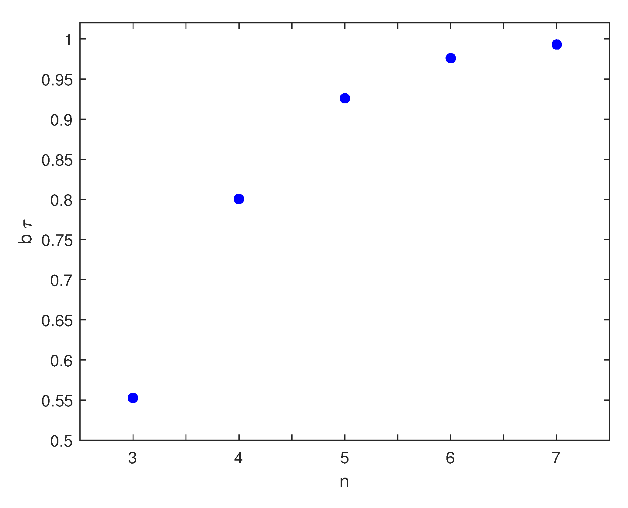
M, a special role is played by the fastest wave that propagates into the equilibrium unperturbed state with the maximum characteristic speed. In all the previous examples, this wave exhibits the fastest decay and the decay coefficient increases when n (and hence M) is increased. We can conjecture that these properties are valid for all RET theories, since a higher number of moments corresponds to a higher number of dissipation terms. In other words, the acceleration waves described by RET balance laws are in perfect agreement with the experimental observations: in a time comparable with the inverse of the relaxation time, the amplitude decreases exponentially and becomes undetectable by a physical measurement apparatus. In fact, no acceleration waves were revealed during experiments. Figure 1 shows the coefficients b of the fastest wave as a function of n. It is easily verified that b increases slowly together with the truncation order.
A distinct general remark has to be addressed to the results concerning the equilibrium characteristic speeds of the different theories. Boillat and Ruggeri have demonstrated a “nesting property” for the characteristic speeds of RET model with an increasing number of moments [19] that we have described in Section 1 and verified in our examples. However, in Section 3, we have found a more peculiar behavior of the spectrum of the equilibrium matrix B | E . In fact, the equilibrium characteristic speeds of an n-system coincide with some equilibrium eigenvalues of the ( n + 2 ) -system. This leads to a distinction between two “families” of systems and their sets of eigenvalues: those for an odd truncation order and those for an even truncation order. We conjecture that this is a general property valid for any n-system and related to the symmetric structure of RET systems of balance laws [10,11,19].

Author Contributions

Conceptualization, F.B. and L.S.; methodology, F.B. and L.S.; validation, F.B. and L.S.; investigation, F.B.; writing—original draft preparation, F.B.; writing—review and editing, F.B. and L.S. All authors have read and agreed to the published version of the manuscript.

Funding

The paper was supported by Gruppo Nazionale di Fisica Matematica (GNFM) dell’INdAM and in part (F.B.) by the Italian research Project PRIN 2017 No. 2017YBKNCE “Multiscale phenomena in Continuum Mechanics: singular limits, off-equilibrium and transitions”.

Conflicts of Interest

The authors declare no conflict of interest.

Appendix A

The present Appendix collects the equation systems and the characteristic polynomials of ET 56 , ET 84 and ET 120 .

Appendix A.1. The ET 56 Case

The one-dimensional set of balance laws is composed now by 12 equations: the first six are the same as (33) 1 6 and we will not write down them here, while the remaining six are given by
ρ ˙ 0 , 2 8 p q ρ 2 x ρ + ( ρ 0 , 2 + 4 ρ 2 , 1 + 20 k B T σ m ) x v 8 k B q m x T + 8 q ρ x σ 20 k B T m x q + x ρ 1 , 2 = 1 τ ρ 0 , 2 ρ ˙ 2 , 1 2 p ( 2 q + ρ 3 , 0 ) ρ 2 x ρ + 2 ρ 4 , 0 + 3 ρ 2 , 1 + 4 p ( 7 p + 5 σ ) 3 ρ x v k B ( 2 q + ρ 3 , 0 ) m x T + 2 ( 2 q + ρ 3 , 0 ) ρ x σ 20 p 3 ρ x q + x ρ 3 , 1 = 1 τ ρ 2 , 1 ρ ˙ 4 , 0 4 p ρ 3 , 0 ρ 2 x ρ + 5 ρ 4 , 0 + 4 p ( 2 p + σ ) ρ x v 4 k B ρ 3 , 0 m x T + 4 ρ 3 , 0 ρ x σ 4 p ρ x q + x ρ 5 , 0 = 1 τ ρ 4 , 0
and
ρ ˙ 1 , 2 + p ρ ρ 0 , 2 4 ρ 2 , 1 + 4 v ( 4 q + 2 ρ 3 , 0 + 2 p v + v σ ) x ρ + + 2 2 ρ 3 , 1 + ρ 1 , 2 + 2 v ( 2 ρ 4 , 0 + 2 ρ 2 , 1 2 q v + ρ 3 , 0 v + 4 p 2 ρ ) x v + + 1 m 3 70 k B 3 T 2 ρ + 2 k B m ( 7 ρ 2 , 1 + k B T ( 4 v 2 ρ + 63 σ ) + 2 m v ( 4 q + 2 ρ 3 , 0 + v σ ) x T + + 1 m 2 ρ 98 k B 2 T 2 ρ + m ( m ρ 0 , 2 + 4 m ρ 2 , 1 4 v ( 4 m q + 2 m ρ 3 , 0 + 2 k B T v ρ + m v σ ) ) x σ + + p ρ x ρ 0 , 2 + 18 p ρ x ρ 2 , 1 = 1 τ ρ 1 , 2 ρ ˙ 3 , 1 k B T m ρ ( 2 ρ 4 , 0 + 3 ρ 2 , 1 ) x ρ + 2 ( ρ 5 , 0 + 2 ρ 3 , 1 ) x v + + 3 k B m 3 m 2 ρ 4 , 0 + m 2 ρ 2 , 1 + 2 k B T ( 7 k B T ρ + 18 m σ ) x T + 75 k B 2 T 2 m 2 + 2 ρ 4 , 0 + 3 ρ 2 , 1 ρ x σ + + 6 k B T m x ρ 2 , 1 + 11 k B T m x ρ 4 , 0 = 1 τ ρ 3 , 1 ρ ˙ 5 , 0 5 k B T ρ 4 , 0 m ρ x ρ + 6 ρ 5 , 0 x v + 10 k B m 3 m 2 ρ 4 , 0 + 3 k B T ( k B T ρ + 3 m σ ) x T + 60 p 2 + 5 ρ ρ 4 , 0 ρ 2 x σ + + 15 k B T m ρ 4 , 0 = 1 τ ρ 5 , 0
After some tedious calculations, the characteristic polynomial can be explicitly written as
P 56 ( λ ˜ ) = k = 0 12 γ k λ ˜ k ,
where
γ 12 = 1 , γ 11 = 0 , γ 10 = 22 k B 2 T m , γ 9 = 0 , γ 8 = 1 3 ρ 2 [ 11 ρ 4 , 0 ρ + 6 ρ ρ 2 , 1 477 p 2 + 108 p σ ] , γ 7 = 1 3 ρ 2 [ 18 ρ ρ 5 , 0 180 p ρ 3 , 0 ] , γ 6 = 1 3 ρ 3 [ 56 p ρ ρ 4 , 0 96 p ρ ρ 2 , 1 + 1404 p 3 1008 p 2 σ ] , γ 5 = 1 3 ρ 3 [ 126 p ρ ρ 5 , 0 + 1260 p 2 ρ 3 , 0 ] , γ 4 = 1 3 ρ 4 [ 360 p 2 ρ ρ 2 , 1 1665 p 4 + 2520 p 3 σ ] , γ 3 = 1 3 ρ 4 [ ( 36 ρ 2 ρ 5 , 0 ρ 2 , 1 + 360 p ρ ρ 2 , 1 ρ 3 , 0 12 ρ 4 , 0 ( 3 ρ 2 ρ 5 , 0 5 ρ 2 ρ 3 , 1 + 15 p ρ ( 2 q + ρ 3 , 0 ) ) + 162 p 2 ρ ρ 5 , 0 1620 p 3 ρ 3 , 0 36 p ( 13 ρ ρ 5 , 0 m 10 ( ρ ρ 3 , 1 6 p q + 4 p ρ 3 , 0 ) ) σ ) ] , γ 2 = 1 3 ρ 5 [ 60 p 3 ρ ρ 4 , 0 360 p 3 ρ ρ 2 , 1 + 810 p 5 2160 p 4 σ ] γ 1 = 1 3 ρ 5 [ 36 p ρ 2 ρ 5 , 0 ρ 2 , 1 360 p 2 ρ ρ 2 , 1 ρ 3 , 0 + 12 p ρ ρ 4 , 0 ( 3 ρ ρ 5 , 0 5 ρ ρ 3 , 1 + + 15 p ( 2 q + ρ 3 , 0 ) ) 54 p 3 ρ ρ 5 , 0 + 540 p 4 ρ 3 , 0 + 36 p 2 ( 13 ρ ρ 5 , 0 10 ( ρ ρ 3 , 1 6 p q + 4 p ρ 3 , 0 ) ) σ ] , γ 0 = 1 3 ρ 6 [ 15 ρ p 4 ρ 4 , 0 + 90 ρ p 4 ρ 2 , 1 135 p 6 + 540 p 5 σ ] .

Appendix A.2. The ET 84 Case

Tedious calculations are required for the one-dimensional PDE system of ET 84 that is composed of 16 equations: the first six are given by (33) 1 6 , the next three are those of (A1), the following three equations are a modification of (A2)
ρ ˙ 1 , 2 + k B T m ρ ρ 0 , 2 4 ρ 2 , 1 + 4 v ( 4 q + 2 ρ 3 , 0 + 2 p v + v σ ) x ρ + + 2 2 ρ 3 , 1 + ρ 1 , 2 + 2 v ( 2 ρ 4 , 0 + 2 ρ 2 , 1 2 q v + ρ 3 , 0 v + 4 p 2 ρ ) x v + + 1 m 3 70 k B 3 T 2 ρ + k B m ( m ρ 0 , 2 4 m ρ 2 , 1 + 4 m v ( 4 q + 2 ρ 3 , 0 + 2 p v + v σ ) x T + + 1 m 2 ρ 35 k B 2 T 2 ρ + m ( m ρ 0 , 2 + 4 m ρ 2 , 1 4 v ( 4 m q + 2 m ρ 3 , 0 + 2 k B T v ρ + m v σ ) ) x σ + + x ρ 2 , 2 = 1 τ ρ 1 , 2 , ρ ˙ 3 , 1 k B T m ρ ( 2 ρ 4 , 0 + 3 ρ 2 , 1 ) x ρ + 2 [ ρ 5 , 0 + 2 ρ 3 , 1 ] x v k B m 2 2 m ρ 4 , 0 + 3 m ρ 2 , 1 + 42 k B T p x T + [ 21 k B 2 T 2 m 2 + 2 ρ 4 , 0 + 3 ρ 2 , 1 ρ ] x σ + x ρ 4 , 1 = 1 τ ρ 3 , 1 , ρ ˙ 5 , 0 5 k B T ρ 4 , 0 m ρ x ρ + 6 ρ 5 , 0 x v 5 k B m 2 m ρ 4 , 0 6 k B T p x T + 15 p 2 + 5 ρ ρ 4 , 0 ρ 2 x σ + x ρ 6 , 0 = 1 τ ρ 5 , 0 ,
while the remaining ones are new with respect to the previous theories:
ρ ˙ 0 , 3 2 k B T m 3 ρ 2 ρ 3 , 1 m 2 + ρ 1 , 2 m 2 + 28 k B 2 T 2 v ρ + 2 v m ( m ρ 0 , 2 2 m ρ 4 , 0 + m ρ 2 , 1 8 m q v + 4 m v ρ 3 , 0 + 4 k B T v 2 ρ + + 2 m v 2 σ ) x ρ + 4 ρ 4 , 1 + 2 ρ 2 , 2 + ρ 0 , 3 8 v ρ 5 , 0 + 4 v ( ρ 3 , 1 + ρ 1 , 2 + 2 v ( 2 ρ 4 , 0 2 ρ 2 , 1 + 2 q v v ρ 3 , 0 ) ) 2 k B 2 T 2 ( 28 k B T ρ + 16 m v 2 ρ 105 m σ ) m 3 x v k B m 3 4 m 2 ρ 3 , 1 25 m 2 ρ 1 , 2 + 56 k b 2 T 2 v ρ + 4 k B m T ( 189 q + 4 ρ v 3 ) + + 4 m 2 v ( ρ 0 , 2 2 ρ 4 , 0 + ρ 2 , 1 + 2 v ( 4 q + 2 ρ 3 , 0 + v σ ) ) x T + 1 m 2 ρ 4 m 2 ρ 3 , 1 + 2 m 2 ρ 1 , 2 + 56 k B 2 T 2 v ρ + + 4 m v ( m ρ 0 , 2 2 m ρ 4 , 0 + m ρ 2 , 1 8 m q v + 4 m v ρ 3 , 0 + 4 k B T v 2 ρ + 2 m v 2 σ ) x σ 588 k B 2 T 2 m 2 x q + 27 k B T m x ρ 1 , 2 = 1 τ ρ 0 , 3 , ρ ˙ 2 , 2 2 k B T m 2 ρ [ 2 m ρ 3 , 1 + m ρ 1 , 2 + 4 v 2 ( 4 m q + 2 m ρ 3 , 0 + 2 k B T v ρ + m v σ ) ] x ρ + [ 4 ρ 4 , 1 + + 1 m 3 ( 3 m 3 ρ 2 , 2 + 84 k B 3 T 3 ρ + 8 m v 2 ( 2 m 2 ρ 4 , 0 2 m 2 ρ 2 , 1 + 2 m 2 q v m 2 v ρ 3 , 0 4 k B 2 T 2 ρ ) + 70 k B 2 m T 2 σ ) ] x v + + k B m 2 [ 18 m ρ 3 , 1 + m ρ 1 , 2 2 k B T ( 108 q + 99 ρ 3 , 0 + 8 v 3 ρ ) 8 m v 2 ( 4 q + 2 ρ 3 , 0 + v σ ) ] x T + + 1 m ρ 4 m ρ 3 , 1 + 2 m ρ 1 , 2 + 8 v 2 ( 4 m q + 2 m ρ 3 , 0 + 2 k B T v ρ + m v σ ) x σ 178 k B 2 T 2 m 2 x q 99 k B 2 T 2 m 2 x ρ 3 , 0 + 3 k B T m x ρ 1 , 2 + 22 k B T m x ρ 3 , 1 = 1 τ ρ 2 , 2 , ρ ˙ 4 , 1 2 k B T m ρ ρ 5 , 0 + 2 ρ 3 , 1 x ρ + 2 ρ 6 , 0 + 5 ρ 4 , 1 + 6 k B 2 T 2 m 3 ( 12 k B T ρ + 7 m σ ) x v + + k B m 2 11 m ρ 5 , 0 + 6 m ρ 3 , 1 20 k B T ( 3 q + 11 ρ 3 , 0 ) x T + 2 ( ρ 5 , 0 + 2 ρ 3 , 1 ) ρ x σ 72 k b 2 T 2 m 2 x q 110 k B 2 T 2 m 2 x ρ 3 , 0 + 10 k B T m x ρ 3 , 1 + 13 k B T m x ρ 5 , 0 = 1 τ ρ 4 , 1 , ρ ˙ 6 , 0 6 k B T ρ 5 , 0 m ρ x ρ + 7 ρ 6 , 0 + 30 k B 2 T 2 ( 2 p + σ ) m 2 x v + 15 k B m 2 m ρ 5 , 0 14 k B ρ 3 , 0 T x T + + 6 ρ 5 , 0 ρ x σ 30 k B 2 T 2 m 2 x q 105 k B 2 T 2 m 2 x ρ 3 , 0 21 k B T m ρ 5 , 0 = 1 τ ρ 6 , 0 .
The corresponding characteristic polynomial is expressed as
P 84 ( λ ˜ ) = λ ˜ 3 k = 0 13 δ k λ ˜ k
where
δ 13 = 1 , δ 12 = 0 , δ 11 = 34 k b 2 T m , δ 10 = 0 , δ 9 = 423 k B 2 T 2 m 2 , δ 8 = 1 3 m ρ 2 [ 13 m ρ ρ 5 , 0 + 10 m ρ ρ 3 , 1 60 p q 220 p ρ 3 , 0 ] , δ 7 = 1 3 m ρ 2 [ 21 m ρ ρ 6 , 0 315 m p ρ 4 , 0 + 7380 k B T p 2 945 k B T p σ ] , δ 6 = 1 3 m ρ 2 [ 102 m p ρ 5 , 0 240 m p ρ 3 , 1 + 1440 k B T p q + 3180 k B T p ρ 3 , 0 ] , δ 5 = 1 3 m 2 ρ 2 [ 273 m 2 p ρ 6 , 0 + 4095 k B T p m ρ 4 , 0 21105 k B 2 T 2 p 2 + 12285 k B 2 T 2 p σ ] , δ 4 = 1 3 m 2 ρ 2 [ 126 k B m T p ρ 5 , 0 + 1680 k B m T p ρ 3 , 1 10080 k B 2 T 2 p q 13860 k B 2 T 2 p ρ 3 , 0 ] , δ 3 = 1 3 m 3 ρ 2 [ 945 k B T m 2 p ρ 6 , 0 14175 k B 2 T 2 m p ρ 4 , 0 + 28350 k B 3 T 3 p 2 42525 k B 3 T 3 p σ ] ,
δ 2 = 1 3 m 6 ρ 2 [ 49 m 6 ρ 5 , 0 ρ 6 , 0 + 105 m 6 ρ 5 , 0 ρ 4 , 1 70 m 6 ρ 6 , 0 ρ 3 , 1 420 m 5 k B T ρ 4 , 0 ρ 5 , 0 + 1050 k B m 5 T ρ 4 , 0 ρ 3 , 1 630 k B m 5 T ρ 5 , 0 ρ 2 , 1 + 420 k B m 5 T q ρ 6 , 0 + 1120 k B m 5 T ρ 3 , 0 ρ 6 , 0 1050 k B m 5 T ρ 3 , 0 ρ 4 , 1 6300 k B 2 T 2 m 4 q ρ 4 , 0 5250 k B 2 m 4 T 2 ρ 3 , 0 ρ 4 , 0 + 6300 k B 2 T 2 m 4 ρ 3 , 0 ρ 2 , 1 + 1470 k B 3 m 3 T 3 ρ ρ 5 , 0 4200 k B 3 m 3 T 3 ρ ρ 3 , 1 + + 25200 k B 4 m 2 T 4 1 ρ q + 23100 k B 4 T 4 m 2 ρ 3 , 0 3465 k B 2 m 4 T 2 σ ρ 5 , 0 + 3150 k B 2 m 4 T 2 σ ρ 3 , 1 18900 k B 3 m 3 T 3 q σ + + 6300 k B 3 m 3 T 3 σ ρ 3 , 0 ] , δ 1 = 1 3 m 6 ρ 2 [ 945 k B 3 m 3 T 3 ρ ρ 6 , 0 + 14175 k B 4 T 4 m 2 ρ ρ 4 , 0 14175 k B 6 T 6 ρ 2 + 42525 k B 5 T 5 m ρ σ ] , δ 0 = 1 3 m 6 ρ 2 [ 147 k B m 5 T ρ 5 , 0 ρ 6 , 0 315 k B m 5 T ρ 5 , 0 ρ 4 , 1 + 210 k B T m 5 ρ 5 , 0 ρ 4 , 1 + 210 k B T m 5 ρ 6 , 0 ρ 3 , 1 + + 1260 k B 2 T 2 m 4 ρ 4 , 0 ρ 5 , 0 3150 k B 2 T 2 m 4 ρ 4 , 0 ρ 3 , 1 + 1890 k B 2 T 2 m 4 ρ 5 , 0 ρ 2 , 1 1260 k B 2 m 4 T 2 q ρ 6 , 0 3360 k B 2 T 2 m 4 ρ 3 , 0 ρ 6 , 0 + + 3150 k B 2 T 2 m 4 ρ 3 , 0 ρ 4 , 1 + 18900 k B 3 m 3 T 3 q ρ 4 , 0 + 15750 k B 3 m 3 T 3 ρ 3 , 0 ρ 4 , 0 18900 k B 3 T 3 m 3 ρ 2 , 1 ρ 3 , 0 1575 k B 4 m 2 T 4 ρ ρ 5 , 0 + + 3150 k B 4 m 2 T 4 ρ ρ 3 , 1 18900 k B 5 T 5 m ρ q 12600 k B 5 m T 5 ρ ρ 3 , 0 + 10395 k B 3 m 3 T 3 σ ρ 5 , 0 9450 k B 3 m 3 T 3 σ ρ 3 , 1 + + 56700 k B 4 T 4 m 2 q σ 18900 k B 4 m 2 T 4 ρ 3 , 0 σ ] .

Appendix A.3. The ET 120 Case

Several calculations are required in order to write down the one-dimensional set of balance laws that is composed of 20 equations: the (33) 1 6 , (A1), (A5) that coincide with equations of previous models, (A10), which is a modification of (A6)
ρ ˙ 0 , 3 2 k B T m 3 ρ ( 2 ρ 3 , 1 m 2 + ρ 1 , 2 m 2 + 28 k B 2 T 2 v ρ + 2 m v ( ρ 0 , 2 m 2 ρ 4 , 0 m + ρ 2 , 1 m 8 m q v + 4 m ρ 3 , 0 v + 4 k B T v 2 ρ + + 2 m v 2 σ ) ) x ρ + ( 4 ρ 4 , 1 + 2 ρ 2 , 1 + ρ 0 , 3 8 ρ 5 , 0 v + 4 v ( ρ 3 , 1 + ρ 1 , 2 + 2 v ( 2 ρ 4 , 0 2 ρ 3 , 1 + 2 q v ρ 3 , 0 v ) ) 8 k B 2 T 2 ( 7 k B T + 4 m v 2 ) ρ ) m 3 + 210 k B 2 T 2 σ m 2 ) x v 1 m 3 2 k B ( 2 ρ 3 , 1 m 2 + ρ 1 , 2 m 2 + 28 k B 2 T 2 v ρ + 2 m v ( ρ 0 , 2 m 2 ρ 4 , 0 m + ρ 2 , 1 m 8 m q v + 4 m ρ 3 , 0 v + 4 k B T v 2 ρ + 2 m v 2 σ ) ) x T + 1 m 2 ρ ( 4 ρ 3 , 1 m 2 + 2 ρ 1 , 2 m 2 + + 56 k B 2 T 2 v ρ + 4 m v ( ρ 0 , 2 m 2 ρ 4 , 0 m + ρ 2 , 1 m 8 m q v + 4 m ρ 3 , 0 v + 4 k B T v 2 ρ + 2 m v 2 σ ) ) x σ 210 k B 2 T 2 m 2 x q + x ρ 1 , 3 = 1 τ ρ 0 , 3 , ρ ˙ 2 , 2 2 k B T ( 2 m ρ 3 , 1 + m ρ 1 , 2 + 4 v 2 ( 4 m q + 2 m ρ 3 , 0 + 2 k B T v ρ + m v σ ) ) m 2 ρ x ρ + + ( . 4 ρ 4 , 1 + 3 ρ 2 , 2 + 1 m 3 ( 84 k B 3 T 3 ρ + 8 m v 2 ( m 2 ( 2 ρ 4 , 0 2 ρ 2 , 1 + 2 q v ρ 3 , 0 v ) 4 k B 2 T 2 ρ ) + 70 k B 2 m T 2 σ ) x v 2 k B ( 2 ρ 3 , 1 m + ρ 1 , 2 m + 4 v 2 ( 4 m q + 2 m ρ 3 , 0 + 2 k B T v ρ + m v σ ) ) m 2 x T + + 4 m ρ 3 , 1 + 2 m ρ 1 , 2 + 8 v 2 ( 4 m q + 2 m ρ 3 , 0 + 2 k B T v ρ + m v σ ) m ρ x σ 70 k B 2 T 2 m 2 x q + x ρ 3 , 2 = 1 τ ρ 2 , 2 , ρ ˙ 4 , 1 ( 2 ( ρ 5 , 0 + 2 ρ 3 , 1 ) k B T ) m ρ x ρ + 2 ρ 6 , 0 + 5 ρ 4 , 1 + 6 k B 2 T 2 ( 12 k B T ρ + 7 m σ ) m 3 x v 2 k B ( ρ 5 , 0 + 2 ρ 3 , 1 ) m x T + 2 ( ρ 5 , 0 + 2 ρ 3 , 1 ) ρ x σ 42 k B 2 T 2 m 2 x q + x ρ 5 , 1 = 1 τ ρ 4 , 1 ρ ˙ 6 , 0 6 ρ 5 , 0 k B T m ρ x ρ + 7 ρ 6 , 0 + 30 k B 2 T 2 ( 2 k T ρ + m σ ) m 3 x v 6 ρ 5 , 0 k B m x T + 6 ρ 5 , 0 ρ x σ 30 k B 2 T 2 m 2 x q + x ρ 7 , 0 = 1 τ ρ 6 , 0 ,
and the four new equations
ρ ˙ 1 , 3 + k B T m 3 ρ ( 6 ρ 2 , 2 m 2 ρ 0 , 3 m 2 + v ( 6 ρ 3 , 1 m 2 6 ρ 1 , 2 m 2 + 70 k B 2 T 2 v ρ + m v ( 5 ρ 0 , 2 m 10 ρ 4 , 0 m + 5 ρ 2 , 1 m 64 m q v + 32 m ρ 3 , 0 v + 32 k B T v 2 ρ + 16 m v 2 σ ) ) ) x ρ + ( 6 ρ 3 , 2 + 2 ρ 1 , 3 + v ( 6 ρ 4 , 1 + 6 ρ 2 , 2 + v ( 10 ρ 5 , 0 5 ( ρ 3 , 1 + ρ 1 , 2 ) + + 32 ( ρ 4 , 0 + ρ 2 , 1 ) v + 16 ( 2 q + ρ 3 , 0 ) v 2 ) + 4 k B 2 T 2 ( 21 k B T + 16 m v 2 ) ρ m 3 ) x v + k B m 4 ( 27 ρ 2 , 2 m 3 594 ρ 2 , 1 k B m 2 T + 6 ρ 3 , 1 m 3 v 6 ρ 1 , 2 m 3 v 10 ρ 4 , 0 m 3 v 2 + 5 ρ 2 , 1 m 3 v 2 64 m 3 q v 3 + 32 m 3 ρ 3 , 0 v 3 + + ρ 0 , 2 m 2 ( 54 k B T + 5 m v 2 ) + 945 k B 3 T 3 ρ + 70 k B 2 m T 2 v 2 ρ + 32 k B m 2 T v 4 ρ 2079 k B 2 m T 2 σ + 16 m 3 v 4 σ ) x T + 1 m 3 ρ ( 6 ρ 2 , 2 m 3 + ρ 0 , 3 m 3 378 k B 3 T 3 ρ m v ( 6 ρ 3 , 1 m 2 6 ρ 1 , 2 m 2 + 70 k B 2 T 2 v ρ + m v ( 5 ρ 0 , 2 m 10 ρ 4 , 0 m + + 5 ρ 2 , 1 m 64 m q v + 32 m ρ 3 , 0 v + 32 k B T v 2 ρ + 16 m v 2 σ ) ) ) x σ 27 k B 2 T 2 m 2 x ρ 0 , 2 297 k B 2 T 2 m 2 x ρ 2 , 1 + k B T m x ρ 0 , 3 + 33 k T m x ρ 2 , 2 = 1 τ ρ 1 , 3 , ρ ˙ 3 , 2 + k B T ( 4 m ρ 4 , 1 3 m ρ 2 , 2 + 12 v 3 ( 4 m q + 2 m ρ 3 , 0 + 2 k B T v ρ + m v σ ) ) m 2 ρ x ρ + 4 ( ρ 5 , 1 + ρ 3 , 2 + 3 v 3 ( 2 ρ 4 , 0 + 2 ρ 2 , 1 2 q v + ρ 3 , 0 v + 4 k B 2 T 2 ρ m 2 ) ) x v + k B m 4 ( 22 ρ 4 , 1 m 3 + 3 ρ 2 , 2 m 3 6 ρ 0 , 2 k B m 2 T 286 ρ 4 , 0 k B m 2 T 264 ρ 2 , 1 k B m 2 T 48 m 3 q v 3 + 24 m 3 ρ 3 , 0 v 3 + 567 k B 3 T 3 ρ + 24 k B m 2 T v 4 ρ 1782 k B 2 m T 2 σ + + 12 m 3 v 4 σ ) x T + 405 k B 3 T 3 m 3 24 k B T v 4 m + 4 ρ 4 , 1 + 3 ( ρ 2 , 2 4 v 3 ( 4 q + 2 ρ 3 , 0 + v σ ) ) ρ x σ 3 k B 2 T 2 m 2 x ρ 0 , 2 132 k B 2 T 2 m 2 x ρ 2 , 1 , 143 k B 2 T 2 m 2 x ρ 4 , 0 + 6 k B T m x ρ 2 , 2 + 26 k B T m ρ 4 , 1 = 1 τ ρ 3 , 2 ,
ρ ˙ 5 , 1 ( 2 ρ 6 , 0 + 5 ρ 4 , 1 ) k B T m ρ x ρ + 2 ( ρ 7 , 0 + 3 ρ 5 , 1 ) x v + + k B ( 13 ρ 6 , 0 m 3 + 5 ( 2 ρ 4 , 1 m 3 + 81 k B 3 T 3 ρ 3 k B m T ( 26 ρ 4 , 0 m + 6 ρ 2 , 1 m + 99 k B T σ ) ) ) m 4 x T 360 k B 3 T 3 m 3 2 ρ 6 , 0 + 5 ρ 4 , 1 ρ x σ 45 k B 2 T 2 m 2 x ρ 2 , 1 195 k 2 T 2 m 2 x ρ 4 , 0 + 15 k B T m x ρ 4 , 1 + 15 k B T m x ρ 6 , 0 = 1 τ ρ 5 , 1 , ρ ˙ 7 , 0 7 ρ 6 , 0 k B T m ρ x ρ + 8 ρ 7 , 0 x v + 21 k B ( ρ 6 , 0 m 3 + 5 k B T ( 4 ρ 4 , 0 m 2 + 3 k B T ( k B T ρ 4 m σ ) ) ) m 4 x T 315 k B 3 T 3 m 3 7 ρ 6 , 0 ρ x σ 210 k 2 T 2 m 2 x ρ 4 , 0 + 28 k B T m x ρ 6 , 0 = 1 τ ρ 7 , 0 .

References

  1. Boillat, G. La Propagation des Ondes; Gauthier-Villars: Paris, France, 1965. [Google Scholar]
  2. Boillat, G.; Ruggeri, T. On the evolution law of weak discontinuities for hyperbolic quasi-linear systems. Wave Motion 1979, 1, 149–152. [Google Scholar] [CrossRef]
  3. Ruggeri, T. Stability and discontinuity waves for symmetric hyperbolic systems. In Nonlinear Wave Motion; Jeffrey, A., Ed.; Longman: London, UK, 1989; pp. 148–161. [Google Scholar]
  4. Truesdell, C.; Noll, W. Handbuch der Physik; Springer: Heidelberg, Germany, 1965; Volume III/3. [Google Scholar]
  5. Muracchini, A.; Ruggeri, T. Acceleration waves, shock formation and stability in a gravitating atmosphere. Astropys. Space Sci. 1989, 153, 127–142. [Google Scholar] [CrossRef]
  6. Müller, I. Extended Thermodynamics: A theory of symmetric hyperbolic field equations. Entropy 2008, 10, 477–492. [Google Scholar] [CrossRef] [Green Version]
  7. Bowen, R.M.; Doria, M.L. Effect of diffusion on the growth and decay of acceleration waves in gases. J. Acoust. Soc. Am. 1973, 53, 75–82. [Google Scholar] [CrossRef]
  8. Muracchini, A.; Seccia, L. Thermo-acceleration waves and shock formation in Extended Thermodynamics of gravitational gases. Contin. Mech. Thermodyn. 1989, 1, 227–237. [Google Scholar] [CrossRef]
  9. Ruggeri, T.; Seccia, L. Hyperbolicity and wave propagation in extended thermodynamics. Meccanica 1989, 24, 127–138. [Google Scholar] [CrossRef]
  10. Müller, I.; Ruggeri, T. Rational Extended Thermodynamics; Springer: New York, NY, USA, 1998. [Google Scholar]
  11. Ruggeri, T.; Sugiyama, M. Rational Extended Thermodynamics beyond the Monatomic Gas; Springer: Basel, Switzerland, 2015. [Google Scholar]
  12. Kogan, M.N. Rarefied Gas Dynamics; Plenum Press: New York, NY, USA, 1969. [Google Scholar]
  13. Grad, H. On the kinetic theory of rarefied gases. Commun. Pure Appl. Math. 1949, 2, 331–407. [Google Scholar] [CrossRef]
  14. Arima, T.; Taniguchi, S.; Ruggeri, T.; Sugiyama, M. Extended thermodynamics of dense gases. Contin. Mech. Thermodyn. 2012, 24, 271–292. [Google Scholar] [CrossRef]
  15. Brini, R.; Ruggeri, T. Entropy principle for the moment systems of degree α associated with the Boltzmann equation. Critical derivatives and non controllable boundary data. Contin. Mech. Thermodyn. 2002, 14, 165–189. [Google Scholar] [CrossRef]
  16. Brini, F.; Ruggeri, T. Second-order approximation of extended thermodynamics of a monatomic gas and hyperbolicity region. Contin. Mech. Thermodyn. 2020, 32, 23–39. [Google Scholar] [CrossRef]
  17. Boillat, G.; Ruggeri, T. Moment equations in the kinetic theory of gases and wave velocities. Contin. Mech. Thermodyn. 1997, 9, 205–212. [Google Scholar] [CrossRef]
  18. Ruggeri, T. Galilean invariance and entropy principle for systems of balance laws. The structure of the extended thermodynamics. Contin. Mech. Thermodyn. 1989, 1, 3–20. [Google Scholar] [CrossRef]
  19. Boillat, G.; Ruggeri, T. Hyperbolic principal subsystem. Entropy convexity and subcharacteritic conditions. Arch. Ration. Mech. Anal. 1997, 137, 305–320. [Google Scholar] [CrossRef]
  20. Bhatnagar, P.L.; Gross, E.P.; Krook, M. A Model for Collision Processes in Gases. I. Small Amplitude Processes in Charged and Neutral One-Component Systems. Phys. Rev. 1954, 84, 511–525. [Google Scholar] [CrossRef]
Figure 1. The coefficient b of the fastest acceleration wave, multiplied by the relaxation time τ is plotted as a function of n. The values were calculated in the previous sections and reported in the previous tables.
Fluids 05 00139 g001
Table 1. The values of a, b and G c r of the acceleration waves propagating with different characteristic velocities.
λ ˜ i | E a i b i G cr
λ ˜ 1 , 2 ( 20 ) | E 2.52727 c 0 0.280584 τ ± 0.111023 c 0 τ
λ ˜ 3 , 4 ( 20 ) | E 0.722222 c 0 0.458333 τ ± 0.634615 c 0 τ
± λ ˜ m a x ( 20 ) = λ ˜ 5 , 6 ( 20 ) | E 1.3862 c 0 0.552749 τ ± 0.398751 c 0 τ
Table 2. The table collects the values of a, b and G c r corresponding to the non-exceptional acceleration waves of ET 35 .
λ ˜ i | E a i b i G cr
λ ˜ 4 , 5 ( 35 ) | E        1.68132 c 0        0.343836 τ        0.204503 c 0 τ
λ ˜ 6 , 7 ( 35 ) | E 0.529238 c 0 0.401235 τ 0.758137 c 0 τ
± λ ˜ m a x ( 35 ) = λ ˜ 8 , 9 ( 35 ) | E 1.53569 c 0 0.800609 τ 0.521334 c 0 τ
Table 3. Values of the coefficients a i and b i , together with the critical value of G ( 0 ) in the case of one-dimensional ET 56 theory.
λ ˜ i | E a i b i G cr
λ ˜ 1 , 2 ( 56 ) | E 0.854423 c 0 0.55994 τ ± 0.655343 c 0 τ
λ ˜ 3 , 4 ( 56 ) | E 0.33333 c 0 0.813333 τ ± 2.44 c 0 τ
λ ˜ 5 , 6 ( 56 ) | E 0.528062 c 0 0.383322 τ ± 0.725904 c 0 τ
λ ˜ 7 , 8 ( 56 ) | E 2.9081 c 0 0.409518 τ ± 0.14082 c 0 τ
λ ˜ 9 , 10 ( 56 ) | E 1.51194 c 0 0.497643 τ ± 0.329141 c 0 τ
± λ ˜ m a x ( 56 ) = λ ˜ 11 , 12 ( 56 ) | E 1.60945 c 0 0.926172 τ ± 0.575458 c 0 τ
Table 4. The values of a, b, and G c r corresponding to the non-exceptional acceleration waves of ET 84 .
λ ˜ i | E a i b i G cr
λ ˜ 5 , 6 ( 84 ) | E 0.642969 c 0 0.519028 τ ± 0.807236 c 0 τ
λ ˜ 7 , 8 ( 84 ) | E 0.3849 c 0 0.797101 τ ± 2.07093 c 0 τ
λ ˜ 9 , 10 ( 84 ) | E 0.497686 c 0 0.38631 τ ± 0.776212 c 0 τ
λ ˜ 11 , 12 ( 84 ) | E 1.82855 c 0 0.435448 τ ± 0.238139 c 0 τ
λ ˜ 13 , 14 ( 84 ) | E 1.49312 c 0 0.688412 τ ± 0.461057 c 0 τ
± λ ˜ m a x ( 84 ) = λ ˜ 15 , 16 ( 84 ) | E 1.69454 c 0 0.97614 τ ± 0.576051 c 0 τ
Table 5. The values of a, b and G c r corresponding to the acceleration waves of ET 120 .
λ ˜ i | E a i b i G cr
λ ˜ 1 , 2 ( 120 ) | E 0.813203 c 0 0.78892 τ ± 0.970139 c 0 τ
λ ˜ 3 , 4 ( 120 ) | E 2.83333 c 0 0.869608 τ ± 0.30692 c 0 τ
λ ˜ 5 , 6 ( 120 ) | E 0.398372 c 0 0.742313 τ ± 1.86337 c 0 τ
λ ˜ 7 , 8 ( 120 ) | E 1.11852 c 0 0.614625 τ ± 0.549497 c 0 τ
λ ˜ 9 , 10 ( 120 ) | E 0.593506 c 0 0.491156 τ ± 0.827551 c 0 τ
λ ˜ 11 , 12 ( 120 ) | E 0.447707 c 0 0.361391 τ ± 0.807203 c 0 τ
λ ˜ 13 , 14 ( 120 ) | E 3.27138 c 0 0.487302 τ ± 0.148959 c 0 τ
λ ˜ 15 , 16 ( 120 ) | E 1.56393 c 0 0.513738 τ ± 0.328492 c 0 τ
λ ˜ 17 , 18 ( 120 ) | E 1.52887 c 0 0.839253 τ ± 0.548936 c 0 τ
± λ ˜ m a x ( 120 ) = λ ˜ 19 , 20 ( 120 ) | E 1.78365 c 0 0.993041 τ ± 0.556746 c 0 τ

