Abstract
This study investigates the effect of an orthogonal-shaped reflecting breakwater on the hydrodynamic characteristics of a vertical cylindrical body. The reflecting walls are placed behind the body, which can be conceived as a floater for wave energy absorption. Linear potential theory is assumed, and the associated diffraction and motion radiation problems are solved in the frequency domain. Axisymmetric eigenfunction expansions of the velocity potential are introduced into properly defined ring-shaped fluid regions surrounding the floater. The hydrodynamic interaction phenomena between the body and the adjacent breakwaters are exactly taken into account by using the method of images. Results are presented and discussed concerning the exciting wave forces on the floater and its hydrodynamic coefficients, concluding that the hydrodynamics of a vertical cylindrical body in front of an orthogonally shaped breakwater differ from those in unbounded waters.
1. Introduction
Coastal environments are the most economically important and intensely used among all areas inhabited by humans [1]. In fact, it has been estimated that nearshore segment is expected to be the largest and fastest growing wave energy market from 2020 to 2025 at a compound annual growth rate of 19.3% [2]. Despite the high energy potential available in offshore waves, several wave energy systems have struggled to commercialize due to their: (a) high costs implicit in the installation, maintenance and connection to the electrical grid; (b) low reliability due to harsh offshore ocean climates; (c) lack of insurability surrounding offshore systems; and (d) potential negative environmental impact at the installation location [3]. Thus, nearshore installations have been happening in almost all the European regions and is a preferred choice by manufacturers owing to the fact that these installations offer better efficiency than onshore ones and easier installations when compared with offshore locations.
To protect and maintain the boundaries of coastal regions, a common practice is to transform, alter and armor shorelines or nearshore areas with a variety of structures, such as seawalls and breakwaters. Breakwaters are widely used structures to reduce the intensity of wave action on the shore. They are barriers that are frequently displaced perpendicularly to the dominant wave direction, which absorb, diffract and reflect part of the wave energy, therefore reducing the amount of energy that reaches shoreline. Within the framework of installing Wave Energy Converters (WECs) nearshore and onshore, so as to use the already developed electric grid, cost efficient solutions may arise by installing WECs in front and/or on existing coastal structures, such as breakwaters.
Previous studies on WEC-breakwater systems highlight how the presence of a breakwater as a sea bottom mounted vertical wall can efficiently enhance the efficiency of the converter. For example, the performance characteristics of an array of five wave energy heaving converters placed in front of a fully reflecting vertical breakwater have been numerically studied in [4], whereas the performance of an array of heaving WECs, coupled with DC generators, in front of a breakwater, were numerically and experimentally investigated in [5]. Similar studies concerning the solution of the corresponding wave diffraction and radiation problems for the case of an arbitrary-shaped floater, in front of a vertical wall, in regular and irregular seas have been presented in the literature [6,7,8,9,10,11]. Furthermore, breakwaters are typically considered as the most suitable and, subsequently, the most researched maritime structures for WEC integration. A number of reviews have been conducted regarding integrated WEC-breakwater systems [12,13,14,15].
With respect to WEC-breakwater system, also floating breakwaters are favored for advantageous reasons such as their relatively low construction costs, reduced dependencies on marine geological conditions, low environmental impact, aesthetic considerations and flexibility [16]. A hybrid system comprising of a WEC arranged in front of a floating pontoon-type breakwater, indicating its amplified efficiency compared to the isolated case has been presented in [17,18,19]. To broaden the effective frequency range of the breakwater-WEC system, a dual pontoon-WEC system consisting of two floating pontoons and two Power Take Off (PTO) systems has been proposed in [20]. In addition, in [21,22] a WEC has been examined, integrated into a floating breakwater, which is supported by a bottom seated structure, moving in heave mode and driving a PTO system to produce power. In [23], a modular floating breakwater system is studied combining the relative motions of the WEC and the breakwater to increase system’s efficiency. Indicative, relevant reviews on other floating WEC-breakwater systems are [24,25,26,27].
As an alternative to reflecting fully protecting breakwaters, permeable breakwaters have already been implemented in the literature, in the form of a pile series [28,29]. Pile breakwaters comprising of one or multiple rows of piles partially attenuate the wave energy due to turbulences and eddies created around piles, preventing also effectively the shore from sediment siltation. The efficiency of pile breakwaters was numerically and experimentally studied by many researchers, e.g., [30,31,32]. Permeable breakwaters also consist of perforated and slotted structures. These porous protection structures are usually bottom seated, operating as permeable breakwaters increasing wave reflection as their porosity decreases [33,34]. As far as WEC-permeable breakwater systems are concerned, the Wave Star [35] can be considered as a WEC-pile breakwater. The machine, a prototype of which has been placed at Nissum Bredning site [36], is equipped with a number of floats which are moved by the waves to activate pumps, the pressure of which drives a hydraulic motor.
In recent decades, apart from vertical fully reflecting—and permeable—breakwaters, semicircular breakwaters have aroused interest in the scientific community based on their advantages compared to conventional vertical walls. Semicircular breakwaters reflect less and transmit more energy than vertical ones at the same relative submerged depth [37,38]. Furthermore, the efficiency of submerged plate breakwaters has been studied parametrically in [39,40]. Parameters such as the effect of wave steepness, the relative depth, the relative submergence and angle of inclination affect the performance of the breakwater. However, these types of breakwaters, to the authors’ knowledge, do not represent wave energy conversion solutions.
In the present study, an orthogonal breakwater type is examined towards, nearshore or onshore wave power absorption efficiency. Two bottom-fixed, vertical, fully reflecting walls of infinite length are assumed, joined at a right angle (i.e., 90 degrees with each other), in an orthogonal configuration. In the area formed by the walls’ angle, an array of WECs can be placed, receiving the benefits from wave reflections on the breakwaters’ walls towards energy performance amplification. The V-shaped arrangements of floaters have been presented in [41,42,43], integrated with Oscillating Water Column devices in the outer and inner area of the formed corner, whereas, in [44,45], a sea-bottom-fixed vertical cylinder in front of two orthogonal walls was studied in terms of its horizontal hydrodynamic forces. In the present contribution the examined vertical cylindrical body can be conceived as a floater for wave energy absorption, based on the heaving device principle. Several distances between the floater and the vertical walls and wave heading angles are studied to investigate the effect of the walls on the body’s hydrodynamic characteristics. The presented theoretical model takes exactly into account the hydrodynamic interaction phenomena between the floater and the reflecting fluid flow in front of the vertical walls, and numerical results are presented in the frequency domain. The corresponding diffraction and motion radiation problems are solved by applying the method of images (i.e., for the effect of the vertical walls) and the method of ‘matched’ eigenfunction expansions (i.e., for the velocity potentials in the fluid domains surrounding the body). The numerous presented results in the form of figures, indicate the significant effect of the reflecting waves from the two walls on the floater’s hydrodynamics. The latter are compared with the corresponding hydrodynamic forces on an isolated WEC (i.e., without the presence of the breakwater) and on a WEC placed in front of a single vertical fully reflecting wall (i.e., single breakwater).
This work is structured as follows: Section 2 describes the applied image method to simulate the effect of the orthogonal breakwater on the floater; Section 3 formulates the diffraction and motion radiation problems, while Section 4 presents the calculation of the hydrodynamic forces on the vertical cylindrical floater based on the image method. In Section 5, numerical results are presented in terms of exciting wave forces and hydrodynamic coefficients. Finally, the conclusions are drawn in Section 6.
2. Breakwater Simulation
A rigid, vertical cylindrical floater, placed in front of two fully reflecting vertical walls, forming a right angle (i.e., 90 degrees), is considered. The walls are rigid, fixed on the sea bottom, with infinite length, extending beyond the undisturbed free surface. The floater is exposed to the action of monochromatic incident waves of linear amplitude H/2 and of circular frequency ω, that propagate at angle β, relative to the horizontal axis x (see Figure 1). In order to describe the fluid flow around the floater in front of the orthogonal breakwaters, the method of images is applied. According to this method, the problem under investigation is equivalent to the one of an array of four floaters consisting of the initial and its image bodies with respect to the two walls that are exposed to the action of surface waves without the presence of the vertical walls. Thus, an equivalent problem of four-directional incident waves is considered: one propagating at angle β, a second one at angle 180-β, a third one at angle 180 + β and a fourth one at angle of 360-β, on an array of four floats, without the presence of the breakwater (see Figure 2). For the solution of the diffraction problem the corresponding results of the four incident wave trains are properly added to produce relevant exciting forces and moments. This is similar for the solution of the radiation problem, where the effect of the image devices on the initial floater’s hydrodynamics is properly taken into consideration (see Section 4).
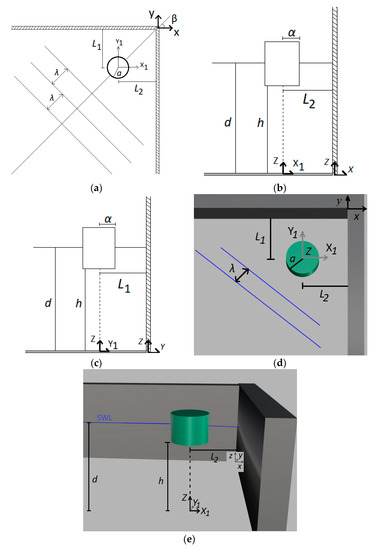
Figure 1.
2-D and 3-D representation of a vertical cylindrical floater in front of an orthogonal breakwater: (a) plan view in 2-D; (b) side view −xz in 2-D; (c) side view −yz in 2-D; (d) plan view −xyz in 3-D; (e) side view −xzy in 3-D.
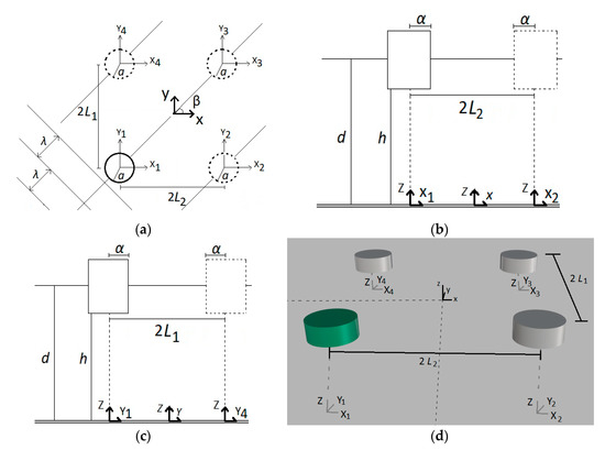
Figure 2.
2-D and 3-D representation of the floaters in the image method: (a) plan view in 2-D; (b) side view −xz in 2-D; (c) side view −yz in 2-D. The image devices are denoted dashed; (d) side view −xyz in 3-D. The image devices are depicted in gray color. The dashed lines in black denote the location of the orthogonal breakwater.
The method of images has been applied in the past to tackle the diffraction and radiation problems of a single or array of cylindrical bodies in channels [46,47,48]. In the present article, it is applied to simulate the effect of two “pure” reflecting walls (i.e., infinite length) on the WEC’s hydrodynamics.
3. Theoretical Modeling
In the present article, a floater of a radius a is considered placed at the inner area formed by the angle of the two breakwaters. The floater is assumed to move only in heave direction; small amplitude heave motions are assumed. The water depth is denoted by d and it is constant, assuming that the sea bottom is flat and horizontal, whereas, the distance between the bottom of the floater and the sea bottom is denoted by h. A global, right-handed Cartesian co-ordinate system O-xyz is introduced with origin located at the sea bottom on the connection point of the two walls, with its vertical axis Oz directed upwards. Moreover, local cylindrical co-ordinate systems are defined with origins at the intersection of the sea bottom with the vertical axis of symmetry of each body (i.e., the initial floater and its image devices—see Section 2). The distance between the walls and the center of the floater is denoted by L1 and L2 (see Figure 1 and Figure 2). The flow is assumed to be incompressible, inviscid and irrotational, whereas, second- or higher-order phenomena are neglected.
In the framework of the linearized potential theory, the fluid flow around the q floater of the arrangement (q = 1, 2, 3, 4, including the initial and its image floaters) can be described by the potential function [4,5,44],
where
In Equation (2), is the undisturbed incident wave component; is the scattered components originating by all floaters of the arrangement, expressed in the co-ordinate system of body q; are the diffraction components; is the radiation component induced around anybody q of the configuration due to the forced oscillation of the p float in the heave direction with unit velocity amplitude; and is the velocity amplitude in heave direction of body p.
The fluid domain is denoted by Ω and extends to infinity, the undisturbed free surface is denoted by SF, which also extends to infinity. The volume of the cylinders is excluded from Ω as well as their cross sections on the undisturbed free surface are excluded from SF. The mean wetted surface of the q body q = 1,…, 4 is denoted by . The underlying boundary value problem is described by the following equations:
where . and g is the gravitational acceleration; is the derivative in the direction of the outward unit normal vector . to the mean wetted surface of the p cylinder; is the Kronecker’s symbol; is the amplitude of the linear heave motion of the q cylinder; and is the generalized normal component.
Furthermore, a radiation condition must be imposed stating that propagating disturbances must be outgoing.
By applying the method of matched axisymmetric eigenfunctions expansions, the flow field around the floaters (i.e., the initial and its image devices) is subdivided in two coaxial ring-shaped fluid regions I, II, i.e., I: and II: , in which different series expansions of the velocity potential can be established. These series representations are solutions of the Laplace equation (see Equation (3)) and satisfy the linearized conditions at the free surface (see Equation (4)); the kinematic condition at the sea bed (see Equation (5)); the kinematic boundary condition at the walls of the floater (see Equations (6) and (7)); and the radiation condition at infinity. Furthermore, the velocity potentials and their derivatives must be continuous at the vertical boundaries of neighboring fluid regions. The associated continuity relations can be written as:
Here, are the velocity potentials of the q cylinder of the array at the I and II fluid regions, respectively.
The velocity potential of the undisturbed incident wave propagating at angles β, 180- β, 180+ β and 360- β can be written as:
with
Here, is the m-th order Bessel function of first kind, k is the wave number related to ω by the dispersion equation; is the distance between the center of the q floater and the origin of the global co-ordinate system; is the angle formed by and the horizontal axis; is defined by
and is its derivative at = d.
In accordance with Equation (10) the diffraction,, and the radiation, , potentials can be obtained as:
The functions are the principal unknowns of the diffraction and radiation problems.
In order to express the potentials in the form of Equations (13) and (14), Twerky’s multiple scattering approach is implemented, taking into consideration the interaction phenomena between the floaters of the array. The method which is applicable to arrays consisting of an arbitrary number of vertical axisymmetric bodies, having any geometrical arrangement and individual body geometry, has been described exhaustively in previous publications [49,50]; thus, it is not further elaborated upon here.
Combining the above, the wave field outside the q cylinder can be written in the below extended form:
Here, is defined by Equation (12), whereas reads
where . are the real roots of
The terms of Equation (15) are presented in Appendix A.
Next, as far as the velocity potential in the lower region II is concerned, , can be written as:
The terms and are presented in Appendix B.
4. Hydrodynamic Forces
Following the solution of the first-order boundary value problem, the exciting wave forces and the hydrodynamic reaction forces acting on the q floater, q = 1,..,4 can be obtained by:
Here is the mean wetted surface of the p floater; ρ is the water density; are the added mass and damping coefficients, respectively, of the q floater in the i-th direction due to the forced oscillation of the p floater in heave direction.
Based on the method of images the exciting forces acting on a vertical cylindrical body in front of an orthogonal breakwater exposed to the action of waves propagating at an angle β, equal to the sum of the exciting forces acting on the initial body, for wave angles β, 180-β, 180+β and 360-β, assuming the presence of image bodies, with respect to the breakwaters, without the presence of the vertical walls. Table 1 summarizes the exciting forces and moments on a vertical cylindrical body in front of an orthogonal breakwater, exposed to the action of a wave train of angle β.

Table 1.
Exciting forces and moments on a vertical cylindrical body in front of an orthogonal breakwater.
In Table 1 the subscripts j = β, 180-β, 180+β, 360-β denote the wave heading angles for each calculated exciting force , i = 1,2,…,5.
Furthermore, the hydrodynamic coefficients in the i-th direction of the initial cylindrical floater due to its own forced oscillation in the heave direction can be derived by summing up properly the motion dependent hydrodynamic coefficients of the initial floater in the i-th direction (i = 1,..,5) due to its forced oscillation in heave direction with the corresponding hydrodynamic coefficients on the initial floater in the i-th direction due to the forced oscillation in heave direction of the image floaters (p = 2,3,4). In Table 2, the formulation for the added mass coefficients is given. The same formula is applied to the damping coefficients.
Table 2.
Hydrodynamic added mass of a vertical cylindrical body in front of an orthogonal breakwater.
5. Numerical Results
5.1. Validation of Results
In order to validate the accuracy of the presented theoretical model, a sea-bottom-fixed vertical cylindrical body located in front of an orthogonal vertical wall is considered in order to compare the results of the present method with the results from Ning et al. [44]. The examined cylinder of radius α is placed at a water depth d/α = 1.0. The distances of the cylinder’s center from the vertical walls are L1 = L2 = 1.5α (see Figure 1, assuming h = 0). Herein, the wave heading angle is β = π/6 (see Figure 1). The dimensionless horizontal exciting forces at x and y direction acting on the vertical cylinder are presented in Figure 3, versus kα. The results are non-dimensionalized by the term of: ρgdαH/2 (i.e., ρ is the water density; g is the acceleration due to gravity; H/2 is the wave amplitude).
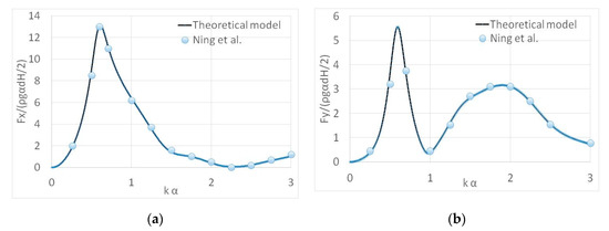
Figure 3.
Horizontal-exciting forces on a bottom fixed cylindrical body placed in front of an orthogonal breakwater using the method of images: (a) horizontal-exciting force on x-axis; (b) horizontal-exciting force on y-axis.
In Figure 3, the outcomes obtained from the present theoretical method are compared with the results from [44] with a very good agreement. More specifically, Figure 3a depicts the exciting forces on the examined bottom fixed cylinder on x-axis, whereas, in Figure 3b, the corresponding forces on the y-axis are depicted. The results from the present analysis concerning the horizontal-exciting forces correlate excellent with the corresponding ones presented in the literature. Therefore, it can be concluded that the present theoretical model can effectively simulate the effect that an orthogonal wall has on the hydrodynamic characteristics of a vertical cylindrical body placed in front of it.
5.2. Test Cases
The method developed herein is applied for a floating vertical cylindrical body in front of an orthogonal (right angle) breakwater (i.e., two bottom-fixed, vertical, reflecting, walls of infinite length is assumed, joined at a right angle, in an orthogonal configuration). The cylindrical floater of radius α, is floating at a water depth d = 3α, whereas, the distance between the floater’s lower surface from the sea bottom equals h = 2α. The distances between the center of the floater and the vertical walls are assumed equal, i.e., L1 = L2 (see Figure 1).
5.2.1. Effect of the Distance between the Walls and the Floater
In this section, the effect of the distance between the walls and the floater is presented, in terms of its exciting forces and hydrodynamic coefficients. The considered distances equal to L1 = L2 = 2α, 4α, 6α, 8α, whereas the wave heading angle is assumed equal to β = π/6 (see Figure 1). The exciting forces, (see Equations (21)–(23)), are non-dimensionalized by the term of ρgα2H/2; the hydrodynamic coefficients, (see Equations (26)–(28)) by the term of ρα3 and the damping coefficient . are non-dimensionalized by the term of ωρα3.
In Figure 4, the dimensionless wave-exciting forces in surge, sway and heave directions (i.e., ) acting on the floater in front of an orthogonal breakwater are plotted against the corresponding values acting on the same floater but in isolation condition (i.e., without the existence of the vertical walls). It is evident that the presence of the vertical walls affects the exciting wave forces at every examined wave number, irrespective of the distance between the floater and the breakwaters, since the forces’ values do not follow the smooth decrease pattern as in the isolated floater’s case. It is depicted that due to the reflected waves from the vertical walls the values of the exciting forces oscillate around those on an isolated floater. Furthermore, it can be seen that, as the distance of the floater from the vertical walls increases, the earlier (i.e., with respect to the wave numbers) the oscillatory behavior of the exciting forces occur. More specifically, when the floater is placed near the walls (i.e., L1 = L2 = 2α) the exciting forces attain higher values, than those of the isolated case, in a wider range of wave numbers (i.e., for the L1 = L2 = 2α case the surge-exciting force have higher values than the isolated case at kα ∈ [0,1.2] and [2.2, 3]). On the other hand, as the distance between the floater and the wall increases, the exciting forces attain local maxima more often but in a narrow wave number range (i.e., for the L1 = L2 = 8α case the surge-exciting force have higher values than the isolated case at kα ∈ [0,0.3]; [0.5,0.85]; [0.95,1.1]; [1.4,1.8]; [2,2.2]; [2.3,2.6]; [2.8,3]). In addition, it is depicted that the exciting forces tend to zero at several wave numbers. This behavior does not appear in the isolated floater case. The zeroing of the exciting forces can be traced back to the interaction phenomena between the floater and the vertical walls. It is also evident from the results that the presence of the vertical walls quadruplicates the heave-exciting forces for wave number tending to zero, regardless the distance between the floater and the vertical walls.
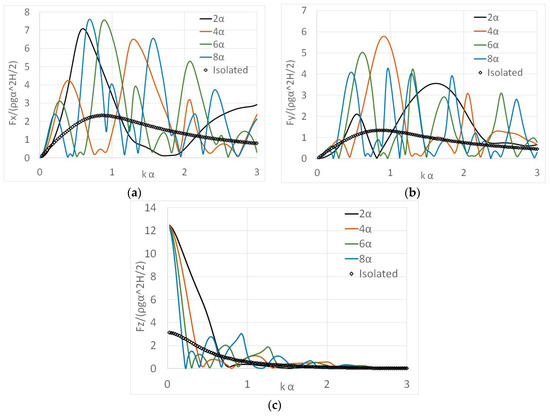
Figure 4.
Exciting forces on a floating cylindrical floater placed in front of an orthogonally shaped (right angle) breakwater using the method of images for L1 = L2 = 2α, 4α, 6α, 8α: (a) horizontal-exciting force on x-axis; (b) horizontal-exciting force on y-axis; (c) vertical-exciting force on z-axis. The results are also compared with the corresponding values of the same isolated floater (i.e., without the presence of the walls).
In Figure 5, the dimensionless hydrodynamic coefficients and are presented, against the corresponding values of the same floater but in isolation condition. The differences between the hydrodynamic coefficients of the floater with and without the presence of the orthogonal walls are evident in the values of the heave hydrodynamic mass and damping coefficients. It is also notable that the hydrodynamic coefficients of the body in front of the orthogonally shaped walls oscillate more rapidly around the corresponding values referred to the isolated body when the distance between the floater and the vertical walls is increasing. A similar conclusion was made for the case of the exciting forces (see Figure 4, and related discussion). Furthermore, in compliance with the behavior of the heave-exciting force in the low wave number regime (Figure 4c), the heave damping coefficients have four times the value of the damping term of an isolated floater for kα tending to zero, regardless the distance between the floater and the walls. As far as the zeroing of the damping coefficients is concerned, this occurs at the same wave numbers where the heave-exciting forces vanish as well. This can be explained on the basis of the Newman-Haskind [51] relations between the damping coefficient and the exciting wave force on a floating body.
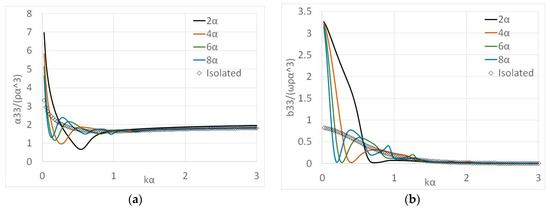
Figure 5.
Hydrodynamic coefficients of a floating cylindrical floater placed in front of an orthogonally shaped (right angle) breakwater using the method of images for L1 = L2 = 2α, 4α, 6α, 8α: (a) heave added mass due to motion of the body in heave; (b) heave damping due to motion of the body in heave. The results are also compared with the corresponding values of the same isolated floater (i.e., without the presence of the walls).
5.2.2. Effect of the Wave Heading Angle
In this section, the effect of the wave heading angle on the floater’s exciting forces is presented. The considered wave heading angles equal to: β = π/6; π/4; π/3; π/2, whereas the distance between the floater and the breakwaters is assumed L1 = L2 = 2α (see Figure 1). For the non-dimensionalizing factor of the exciting forces, the reader is referred to Section 5.2.1.
In Figure 6, the dimensionless wave-exciting forces in surge, sway, heave directions (i.e., ) acting on the floater, when placed in front of an orthogonally shaped breakwater, for several examined wave heading angles β are plotted. Due to symmetry, the surge-exciting force for β = π/6 equals the sway-exciting force for β = π/3 (and vice versa). Similarly, the heave-exciting forces for β = π/6; π/3 are equal. The results of Figure 6 depict that for kα < 1, the surge horizontal-exciting forces increase as the wave heading angle decreases. On the other hand, for the same wave number range (i.e., kα < 1) the sway-exciting forces evidently increase as the wave train angle also increases. It can be also seen that the sway-exciting forces attain their maximum values for β = π/2 at 0 < kα < 1.2 and 1.8 < kα < 2.8 (i.e., due to symmetry the surge-exciting forces attain their maximum values, also for the same wave number ranges, but for β = 0). As far as the wave heading angle β = π/3 is concerned, it can be seen that the surge-exciting forces attain maximum values at 1.2 < kα < 1.8 (i.e., similar due to symmetry for the wave heading angle β = π/6 and the sway-exciting values).
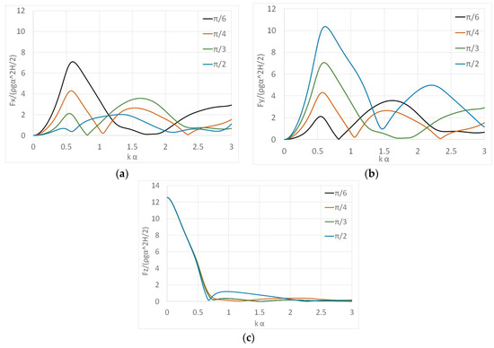
Figure 6.
Exciting forces on a floating cylindrical floater placed in front of an orthogonally (right angle) breakwater using the method of images for β = π/6; π/4; π/3; π/2: (a) horizontal-exciting force on x-axis; (b) horizontal-exciting force on y-axis; (c) vertical-exciting force on z-axis.
Concerning the heave-exciting forces it can be seen that they attain similar values at 0 < kα < 0.6, regardless the examined wave heading angles, whereas, at 0.6 < kα < 2, the heave forces maximize for wave angle β = π/2 (i.e., also for β = 0 for symmetry reasons). The heave-exciting forces minimize at kα ≈ 0.775. This wave number corresponds to a wavelength equal to twice the distance between the initial and the image floater [52].
5.2.3. Effect of the Floater’s Draught
The effect of the floater’s draught on its hydrodynamic characteristics is examined in the present section. Several floater’s draughts are examined i.e., α/h = 0.4; 0.5; 0.66; 1.0 (see Figure 1). The considered distance between the floater and the vertical walls equals L1 = L2 = 2α, whereas the wave heading angle is assumed equal to β = π/6. For the non-dimensionalizing factor of the exciting forces and hydrodynamic coefficients, the reader is referred to Section 5.2.1.
In Figure 7, the horizontal and vertical-exciting forces applied on the examined floater are presented for several floater’s draughts α/h. From the depicted results, it is obvious that the increase of the floater’s draught leads to an increase of the horizontal-exciting forces (in surge and sway direction). This increase is strongly dependent on the floater’s wetted surface. In particular, the larger the draught of the floater is, the more pronounced are the horizontal-exciting forces. It is noted that the exciting forces in surge direction increase quite rapidly up to kα ≈ 0.6, where they attain their global maximum, and then decrease attaining their minimum values at 1.6 < kα < 1.9, regardless of the examined draught values. Similar, the sway-exciting forces attain two local maxima at kα ≈ 0.5; 1.6 and a global minimum at 0.75 < kα < 0.85. It is worthwhile to note that, as the draught increases, the observed minimization of the sway-exciting force is shifted at slightly lower values of kα.
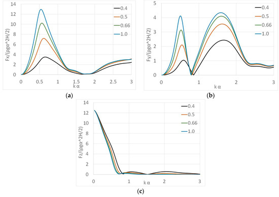
Figure 7.
Exciting forces on a floating cylindrical floater placed in front of an orthogonally shaped (right angle) breakwater using the method of images for a/h = 0.4; 0.5; 0.66; 1.0: (a) Horizontal-exciting force on x-axis; (b) Horizontal-exciting force on y-axis; (c) Vertical-exciting force on z-axis.
On the other hand, the heave-exciting forces decrease with the increase of the floater’s draught (see Figure 7c). For all the examined draughts the heave-exciting forces have a value four times higher than the corresponding one of the no-wall case (see also Figure 4 and related discussion) at small wave numbers (i.e., for kα tending to zero). A rapid decrease is also observed up to 0.6 < kα < 0.8, where the heave force attains minimum values. The observed minimum values are shifted to lower wave numbers as the floater draughts increase.
Figure 8 depicts the heave added mass and the heave hydrodynamic damping coefficients of the examined floater due to its motion in heave direction for several examined draughts. It can be seen that the draught of the floater affects the added mass of the heaving device since higher values of added mass are obtained for larger floater’s draughts. As far as the heave hydrodynamic damping coefficients is concerned, their values increase as the draught of the floater decreases. Furthermore, the damping coefficients values are four time larger than those of the no wall case (see also Figure 5c and relative discussion) for small wave numbers. In addition, the wave numbers where the heave damping coefficients minimize are the same with those that minimize the heave-exciting forces (see also Figure 7c).
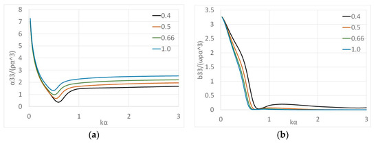
Figure 8.
Hydrodynamic coefficients of a floating cylindrical floater placed in front of an orthogonally shaped (right angle) breakwater using the method of images for a/h = 0.4; 0.5; 0.66; 1.0: (a) heave added mass due to motion of the floater in heave (b) heave damping due to motion of the floater in heave.
In Figure 9, the surge-added mass, and the surge hydrodynamic damping coefficients, of the examined floater due to its motion in heave direction are presented for the examined draughts. Regarding the surge-added mass (Figure 9a), it can be seen that it attains negative values at small wave numbers, whereas, from kα > 0.5 its values are increased up to kα ≈ 0.6 where the surge-added mass attains its maximum value. As far as the surge damping coefficient is concerned, it can be seen that irrespectively of the floater’s draught the surge damping receives negative values at small wave numbers (i.e., kα < 0.75), whereas, a rapid decrease of the damping values is noted up to kα ≈ 0.5. This decrease is more pronounced in the large-draught cases (i.e., α/h = 1.0; 0.66). For all the examined floater’s draught, the surge damping coefficients attain positive maximum values at kα > 0.75 with successively decreasing values towards higher wave numbers. This maximum is shifted at slightly lower values of kα as the floater’s draught increases.
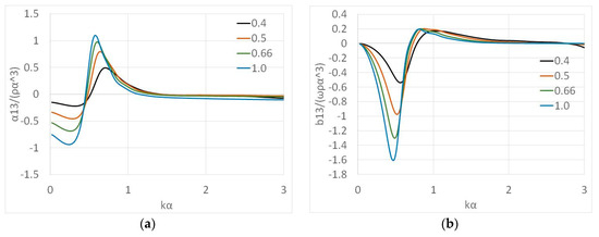
Figure 9.
Hydrodynamic coefficients of a floating cylindrical floater placed in front of an orthogonally shaped breakwater using the method of images for a/h = 0.4; 0.5; 0.66; 1.0: (a) surge-added mass due to motion of the body in heave (b) surge damping coefficient due to motion of the body in heave.
5.2.4. Effect of the Breakwater Type
In the present section the results of the examined configuration (i.e., a floater in front of an orthogonally shaped breakwater) are compared with the corresponding ones of the same floater placed in front of a linear bottom mounted, fully reflecting, vertical wall [8,9]. Concerning the orthogonally shaped breakwater case, the floater is assumed to have a draught equals α/h = 0.5, whereas its distance from the vertical walls equals L1 = L2 = 2α (see Figure 1). As far as the linear-breakwater case is concerned, the same floater is considered in front of an infinite length wall, which is placed along the y axis. The distance between the floater and the vertical wall equals L = 2α (see Figure 10). In both examined configurations, the wave heading angle, relative to the horizontal axis x, equals β = π/6. The non-dimensionalizing factor of the exciting forces and hydrodynamic coefficients is presented to Section 5.2.1.
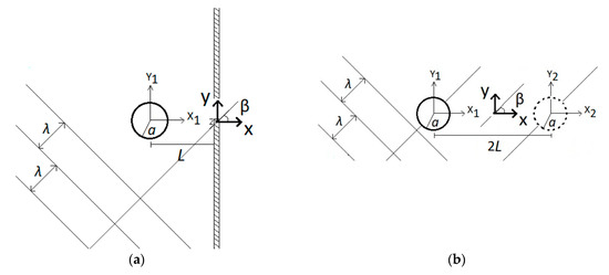
Figure 10.
2-D representation of a vertical cylindrical floater in front of a linear vertical breakwater: (a) plan view of the floater-breakwater system; (b) floaters’ representation in the image method (the image device is denoted dashed).
Figure 11 and Figure 12 depict the surge, sway, heave-exciting forces and heave hydrodynamic coefficients, respectively, of the described floater when the latter is placed in front of a linear breakwater. The results are compared with the corresponding values of the right-angle breakwater case and the isolated case.
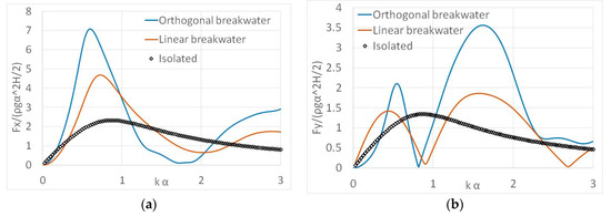
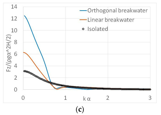
Figure 11.
Exciting forces on a floating cylindrical floater placed in front of a linear breakwater using the method of images: (a) horizontal-exciting force on x-axis; (b) horizontal-exciting force on y-axis; (c) vertical-exciting force on z-axis. The results are compared with the corresponding values of the same floater placed in front of a right-angle-shaped breakwater and in isolation condition (i.e., without the presence of the breakwater).
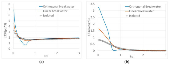
Figure 12.
Hydrodynamic coefficients of a floating cylindrical floater placed in front of a linear breakwater using the method of images: (a) heave added mass due to motion of the floater in heave (b) heave damping coefficient due to motion of the floater in heave. The results are compared with the corresponding values of the same floater placed in front of an orthogonal breakwater and in isolation condition (i.e., without the presence of the breakwater).
The results of Figure 11 demonstrate clearly that when the floater is placed in front of an orthogonal breakwater, the oscillatory behavior of the horizontal-exciting forces is more pronounced. In particular, the values of the surge and sway-exciting forces are oscillating around the corresponding values of the single-breakwater case. This is not the case for the heave-exciting forces since a similar variation pattern is observed for the values of the heave forces in both breakwater cases (i.e., orthogonally shaped and linear). However, at small wave numbers, the heave-exciting forces on the floater in front of an orthogonal breakwater attain twice values than the corresponding forces on the same floater in front of a single breakwater. As far as the heave hydrodynamic coefficients are concerned, it can be seen in Figure 12 that, for the small wave numbers, the hydrodynamic coefficients in both breakwaters cases attain larger values than the isolated case up to kα ≈ 0.2 and 0.6 for the added mass and damping coefficients, respectively.
However, by successively increasing the wave number, the hydrodynamic coefficients decrease up to kα ≈ 1, where both the breakwater cases and the isolated case depict comparable results.
5.2.5. Effect of the Length of the Walls
In the applied image method, the orthogonal breakwater is assumed as a pure reflecting wall of infinite length. Thus, the effect of the length of the walls on the exciting forces and hydrodynamic coefficients of the floater in front of an orthogonal breakwater is presented herein. The theoretical outcomes from the method of images for an orthogonal breakwater of infinite length are compared with the corresponding numerical results derived from the analysis of an orthogonal breakwater of finite length. For the latter analysis, a panel numerical software HAQi [53] has been applied to the cylinder breakwater system. The examined floater is assumed to have a radius α; draught equals α/(d − h) = 2, whereas, its distance from the vertical walls equals L1 = L2 = 2α (see Figure 1). The water depth equals d = 1.5α. As far as the length of each vertical wall in the finite orthogonal breakwater case, it is assumed equal to 40α. In both examined configurations (i.e., infinite and finite breakwater) the wave heading angle equals β = π/6. The non-dimensionalizing factor of the exciting forces and hydrodynamic coefficients is presented to Section 5.2.1.
Figure 13 and Figure 14 depict the surge, sway, heave-exciting forces and heave and surge hydrodynamic coefficients, respectively, of the described floater when the latter is placed in front of an orthogonal breakwater of finite length. The results are compared with the corresponding values of the orthogonal breakwater case of infinite length.
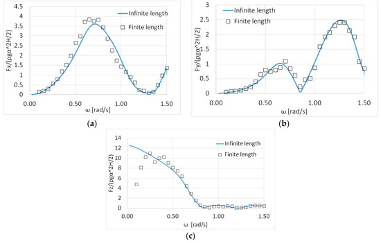
Figure 13.
Exciting forces on a floating cylindrical floater placed in front of an orthogonal breakwater of finite length: (a) horizontal-exciting force on x-axis; (b) horizontal-exciting force on y-axis; (c) vertical-exciting force on z-axis. The results are compared with the corresponding values of the same floater placed in front of an infinite length orthogonal breakwater.
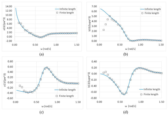
Figure 14.
Hydrodynamic coefficients of a floating cylindrical floater placed in front of an orthogonal breakwater of finite length: (a) heave added mass due to motion of the floater in heave (b) heave damping coefficient due to motion of the floater in heave (c) surge-added mass due to motion of the floater in heave (d) surge damping coefficient due to motion of the floater in heave. The results are compared with the corresponding values of the same floater placed in front of an infinite length orthogonal breakwater.
It can be seen from Figure 13 that the surge and sway-exciting forces for finite-length breakwaters agree quite well with the ones obtained for the infinite-length vertical walls. It should be noted, however, that discrepancies between these two cases do appear and, therefore, the infinite wall assumption simulated theoretically by the method of images should be used with care. As far as the heave-exciting forces is concerned, the consideration of a “pure” wave reflection in the infinite-length case causes an overestimation of the values of the forces at small wave frequencies. More specifically, for the examined finite-length wall case, the values of Fz start their variation close to the limiting value of π (at ω = 0.05 rad/s). On the other hand, the heave-exciting forces on the floater, using the image method (i.e., infinite wall-length), attain four times higher values at small wave frequencies (i.e., ω = 0.05 rad/s).
Regarding the heave and surge-added mass of the floater presented in Figure 14a,c and the surge damping coefficient depicted in Figure 14d, both cases (i.e., finite and infinite wall length) attain similar results. Few discrepancies do appear (i.e., at ω < 0.2 rad/s). However, discrepancies are more intense in the case of the heave damping coefficients (see Figure 14b) and especially for small wave frequencies (i.e., ω < 0.4 rad/s), where the infinite wall assumption overestimates the results of the corresponding heave damping coefficient compared to the ones of the finite length case.
6. Conclusions
This study deals with the determination of the hydrodynamic loads on a vertical cylindrical floater placed in front of an orthogonal breakwater. The image method is applied, assuming walls of infinite length, to simulate the effect of the breakwater on the floater’s characteristics. Furthermore, the multiple scattering approach has been used to evaluate the interaction phenomena between the initial floater and its image bodies.
Several distances between the floater and the vertical walls; floater’s draughts and wave heading angles have been investigated. Based on the theoretical computations shown and discussed in the dedicated sections, the main findings of the present research contribution concern the effect of the breakwater on the exciting wave forces and the hydrodynamic coefficients of the floater at every examined wave number, which should not be neglected when designing a WEC in front of an orthogonal breakwater. This effect—the significance of which is depending on the distance of the floater’s from the vertical walls, its draught and the angles of the wave train—causes an increase or decrease of the floater’s hydrodynamic forces at specific wave numbers compared to their isolated body results. Additionally, it is shown that the effect of the examined orthogonal breakwater affects considerably the device’s hydrodynamics compared to their corresponding values for the linear breakwater case and the no-wall case.
Furthermore, from the comparisons between the finite length breakwater case and its infinite counterpart, it can be obtained that the accuracy of the hydrodynamic forces on a floater in front of an infinite length breakwater has limitations, especially in the low wave number band. These discrepancies between the two configurations (i.e., finite and infinite breakwater length) can be traced back to the pure wave reflecting assumption of the applied image method for the infinite breakwater length which leads to an overestimation of the aforementioned physical quantities.
In conclusion, the effect of an orthogonal breakwater on the exciting wave forces and hydrodynamic coefficients of a floater, when the latter is placed in front of the walls, increases or decreases depending on the distance of the floater from the walls, the geometric characteristics of the floater, the wave heading angle and the length of the vertical walls. Nevertheless, the present research will be continued further by determining in detail the power efficiency of a WEC placed in front of a V-shaped breakwater of an arbitrary forming angle between the vertical walls.
Author Contributions
Conceptualization, S.A.M.; methodology, S.A.M., D.N.K.; software, S.A.M. validation, D.N.K.; S.A.M.; formal analysis, D.N.K.; investigation, S.A.M., D.N.K.; writing—original draft preparation, D.N.K.; writing—review and editing, S.A.M.; supervision, S.A.M.; project administration, S.A.M. All authors have read and agreed to the published version of the manuscript.
Funding
This research received no external funding.
Conflicts of Interest
The authors declare no conflict of interest.
Appendix A
The terms of Equation (15) for the outer fluid domain I: read
where
In (A1), is the mth order Bessel function of first kind; is the mth order Hankel function of first kind, whereas, in (A2) is the mth order modified Bessel function of first kind; and is the modified Bessel function of the second type. Also, are the real roots of Equation (17) and k is the wave number.
In (A4), are Fourier coefficients of the q converter for the outer fluid domain I, determined by the solution of p converter’s forced oscillation. The terms are Fourier coefficients in the I fluid domain, when the converter p is assumed isolated in the water field, determined by the solution of its forced oscillation problem. Furthermore, are Fourier coefficients derived by the diffraction problem in the outer fluid domain [49,50,54]. The term is presented in [50] (Equation (31))[M1] ; p. 495).
Appendix B
The terms presented in Equation (18) can be written as
Here, is the mth order modified Bessel function of first kind.
The terms of Equation (18) equal to
Here, are Fourier coefficients of the q converter for the lower fluid domain II, determined by the solution of p converter’s forced oscillation. Additionally, are Fourier coefficients in the II fluid domain, when the converter p is assumed isolated in the water field, determined by the solution of its forced oscillation problem. Furthermore, are Fourier coefficients derived by the diffraction problem in the lower fluid domain [49,50,54].
References
- Vona, I.; Gray, M.W.; Nardin, W. The impact of submerged breakwaters on sediment distribution along marsh boundaries. Water 2020, 12, 1016. [Google Scholar] [CrossRef]
- Wave Energy Market by Technology (OSW, OBC, & Overtopping Converters), Location (Onshore, Nearshore, Offshore), Application (Desalination, Power Generation, and Environmental Protection), and Region—Global Forecast to 2025; Research and Markets ID: 5011806. Available online: https://www.researchandmarkets.com/ (accessed on 13 August 2020).
- MacGillivray, A.; Jeffrey, H.; Hanmer, C.; Magagna, D.; Raventos, A.; Badcock-Broe, A. Ocean Energy Technology: Gaps and Barriers. Si Ocean, 2013. Available online: www.si-ocean.eu (accessed on 1 May 2020).
- Mavrakos, S.A.; Katsaounis, G.M.; Nielsen, K.; Lemonis, G. Numerical performance investigation of an array of heaving wave power converters in front of a vertical breakwater. In Proceedings of the 14th International Offshore and Polar Engineering Conference (ISOPE 2004), Toulon, France, 23–28 May 2004. [Google Scholar]
- Mavrakos, S.A.; Katsaounis, G.M.; Kladas, A.; Kimoulakis, N. Numerical and experimental investigation of performance of heaving WECs coupled with DC generators. In Proceedings of the 9th European Wave and Tidal Energy Conference, Southampton, UK, 5–9 September 2011. [Google Scholar]
- Teng, B.; Ning, D.Z. Wave diffraction from a uniform cylinder in front of a vertical wall. Ocean Eng. 2003, 21, 48–52. [Google Scholar]
- Teng, B.; Ning, D.Z.; Zhang, X.T. Wave radiation by a uniform cylinder in front of a vertical wall. Ocean Eng. 2004, 31, 201–224. [Google Scholar] [CrossRef]
- Zheng, S.; Zhang, Y. Wave diffraction from a truncated cylinder in front of a vertical wall. Ocean Eng. 2015, 104, 329–343. [Google Scholar] [CrossRef]
- Zheng, S.; Zhang, Y. Wave radiation from a truncated cylinder in front of a vertical wall. Ocean Eng. 2016, 111, 602–614. [Google Scholar] [CrossRef]
- Schay, J.; Bhattacharjee, J.; Soares, C. Numerical modelling of a heaving point absorber in front of a vertical wall. In Proceedings of the 32nd International Conference on Ocean, Offshore and Artic Engineering (OMAE 2013), Nantes, France, 9–14 June 2013. [Google Scholar] [CrossRef]
- Loukogeorgaki, E.; Boufidi, I.; Chatjigeorgiou, I. Performance of an array of oblate spheroidal heaving wave energy converters in front of a wall. Water 2020, 12, 188. [Google Scholar] [CrossRef]
- Zhao, X.L.; Ning, D.Z.; Liang, D.F. Experimental investigation on hydrodynamic performance of a breakwater-integrated WEC system. Ocean Eng. 2019, 171, 25–32. [Google Scholar] [CrossRef]
- Rosa-Santos, P.; Taveira-Pinto, F.; Clemente, D.; Cabral, T.; Fiorentin, F.; Belga, F.; Morais, T. Experimental Study of a Hybrid Wave Energy Converter Integrated in a Harbor Breakwater. J. Mar. Sci. Eng. 2019, 7, 18. [Google Scholar] [CrossRef]
- Cabral, T.; Clemente, D.; Rosa-Santos, P.; Taveira-Pinto, F.; Morais, T.; Belga, F.; Cestaro, H. Performance Assessment of a Hybrid Wave Energy Converter Integrated into a Harbor Breakwater. Energies 2020, 13, 236. [Google Scholar] [CrossRef]
- Cascajo, R.; Garcia, E.; Quiles, E.; Correcher, A.; Morat, F. Integration of marine wave energy converters into seaports: A case study in the port of Valencia. Energies 2019, 12, 787. [Google Scholar] [CrossRef]
- Zhao, X.L.; Ning, D.Z.; Zou, Q.P.; Qiao, D.S.; Cai, S.Q. Hybrid floating breakwater-WEC system: A review. Ocean Eng. 2019, 186, 106126. [Google Scholar] [CrossRef]
- Zhao, X.L.; Ning, D.Z.; Zhang, C.W.; Liu, Y.Y.; Kang, H.G. Analytical study on an oscillating buoy wave energy converter integrated into a fixed box-type breakwater. Math. Probl. Eng. 2017, 2017, 1–9. [Google Scholar] [CrossRef]
- Zhao, X.L.; Ning, D.Z.; Zhang, C.W.; Kang, H.G. Hydrodynamic investigation of an oscillating buoy wave energy converter integrated into a pile-restrained floating breakwater. Energies 2017, 10, 712. [Google Scholar] [CrossRef]
- Zhao, X.; Ning, D. Experimental investigation of breakwater type wec composed of both stationary and floating pontoons. Energy 2018, 155, 226–233. [Google Scholar] [CrossRef]
- Ning, D.; Zhao, X.; Zhao, M.; Hann, M.; Kang, H. Analytical investigation of hydrodynamic performance of a dual pontoon WEC-type breakwater. Appl. Ocean Res. 2017, 65, 102–111. [Google Scholar] [CrossRef]
- Ning, D.; Zhao, X.; Goteman, M.; Kang, H. Hydrodynamic performance of a pile restrained wec-type floating breakwater: An experimental study. Renew. Energy 2016, 95, 531–541. [Google Scholar] [CrossRef]
- Madhi, F.; Yeung, R.W.; Sinclair, M.E. The “Berkeley Wedge”: An asymmetrical energy-capturing floating breakwater of high performance. Mar. Syst. Ocean Technol. 2014, 9, 5–16. [Google Scholar] [CrossRef]
- Zingale, G. Modular Floating Breakwater of the Transformation of Wave Energy. U.S. Patent No. 6,443,653, 3 September 2002. [Google Scholar]
- Martinelli, L.; Ruol, P.; Favaretto, C. Hybrid structure combining a wave energy converter and a floating breakwater. In Proceedings of the International Offshore and Polar Engineering Conference, Rhodes, Greece, 26 June–1 July 2016; pp. 622–628. [Google Scholar]
- Favaretto, C.; Martinelli, L.; Ruol, P.; Cortellazzo, G. Investigation on possible layouts of a catamaran floating breakwater behind a wave energy converter. In Proceedings of the International Ocean and Polar Engineering Conference, San Francisco, CA, USA, 25–30 June 2017. [Google Scholar]
- Chen, B.; Ning, D.; Liu, C.; Greated, C.; Kang, H. Wave energy extraction by horizontal floating cylinders perpendicular to wave propagation. Ocean Eng. 2016, 121, 112–122. [Google Scholar] [CrossRef]
- Michailides, C.; Angelides, D. Wave energy production by a flexible floating breakwater. In Proceedings of the International Offshore and Polar Engineering Conference, Maui, HI, USA, 19–24 June 2011; pp. 614–621. [Google Scholar]
- Sundar, V.; Subbarao, B.V.V. Hydrodynamic performance characteristics of quadrant front face pile supported breakwater. J. Waterw. PortCoast. Ocean Eng. 2003, 129, 22–33. [Google Scholar] [CrossRef]
- Suh, K.D.; Jung, H.Y.; Pyun, C.K. Wave reflection and transmission by curtain wall-pile breakwaters using circular piles. J. Waterw. PortCoast. Ocean Eng. 2007, 34, 2100–2106. [Google Scholar] [CrossRef]
- Hu, P. Dynamic responses analysis of permeable breakwater subjected to random waves. Adv. Mater. Res. 2015, 1061, 809–812. [Google Scholar]
- Elkotby, M.; Rageh, O.; Sarhan, T.; Ezzeldin, M. Wave transformation behind permeable breakwater. Int. J. Sci. Eng. Res. 2019, 10, 83–90. [Google Scholar] [CrossRef]
- Yoo, J.; Kim, S.-Y.; Kim, J.-M.; Cho, Y.-S. Experimental Investigation of the Hydraulic Performance of Caisson-Pile Breakwaters. J. Coast. Res. 2010, 263, 444–450. [Google Scholar] [CrossRef]
- Pourteimouri, P.; Hejazi, K. Development of An Integrated Numerical Model for Simulating Wave Interaction with Permeable Submerged Breakwaters Using Extended Navier–Stokes Equations. J. Mar. Sci. Eng. 2020, 8, 87. [Google Scholar] [CrossRef]
- Mellink, B.A. Numerical and Experimental Research of Wave Interaction with a Porous Breakwater. Master’s Thesis, Faculty of Civil Engineering and Geosciences TU Delft, Delft, The Netherlands, 2012. [Google Scholar]
- Wave Star Energy. Available online: www.wavestarenergy.dk (accessed on 13 August 2020).
- Steenstrup, P.R. Wave Star Energy—New wave energy converter, which is now under going sea trial in Denmark. In Proceedings of the International Conference Ocean Energy, Bremerhaven, Germany, 23–24 October 2006. [Google Scholar]
- Jiang, X.L.; Zou, Q.P.; Zhang, N. Wave load on submerged quarter-circular and semicircular breakwaters under irregular waves. Coast. Eng. 2017, 121, 265–277. [Google Scholar] [CrossRef]
- Gomes, A.; Pinho, J.; Valante, T.; Antuanes do Carmo, J.; Hegde, A.V. Performance assessment of a semi-circular breakwater through CFD modelling. J. Mar. Sci. Eng. 2020, 8, 226. [Google Scholar] [CrossRef]
- Rao, S.; Shirlal, K.G.; Varghese, R.V.; Govindaraja, K.R. Physical model studies on wave transmission of a submerged inclined plate breakwater. Ocean Eng. 2009, 36, 1199–1207. [Google Scholar] [CrossRef]
- Shirlal, K.G. Wave transmission of submerged inclined serrated plate breakwater. Int. J. Chem. Environ. Biol. Sci. 2013, 1, 657–660. [Google Scholar]
- Retief, G.; Muller, F.; Prestedge, G. Detailed design of a wave energy conversion plant. In Proceedings of the 19th Conference on Coastal Engineering, Houston, TX, USA, 19 November 1984. [Google Scholar]
- Kelly, T.; Dooley, T.; Campbell, J.; Ringwood, J.V. Comparison of the experimental and numerical results of modelling a 32-oscillating water column, V-shaped floating wave energy converter. Energies 2013, 6, 4045–4077. [Google Scholar] [CrossRef]
- Ackerman, P.H. Air Turbine Design Study for a Wave Energy Conversion System. Master’s Thesis, Department of Mechanical and Mechatronic Engineering, University of Stellenbosch, Stellenbosch, South Africa, 2009. [Google Scholar]
- Ning, D.; Teng, B.; Song, X. Analytical study on wave diffraction from a vertical circular cylinder in front of orthogonal vertical walls. Mar. Sci. Bull. 2005, 7, 1. [Google Scholar]
- Ning, D.; Teng, B. Study on the oscillation of a uniform cylinder in front of two vertical walls intersecting normally. Chin. Eng. Sci. 2003, 5, 84–91. [Google Scholar]
- Spring, B.W.; Monkmeyer, P.L. Interaction of plane waves with a row of cylinders. In Proceedings of the 3rd Specialty Conference of Civil Engng in Oceans, ASCE, Newark, DE, USA, 9–12 June 1975; pp. 979–998. [Google Scholar]
- Yeung, R.W.; Sphaier, S.H. Wave-interference effects on a truncated cylinder in a channel. J. Eng. Math. 1989, 23, 95–117. [Google Scholar] [CrossRef]
- Mavrakos, S.A. The scattered wave field by vertical cylinders in a narrow tank. In Proceedings of the 4th National Symposium on Theoretical and Applied Mechanics, Xanthi, Greece, 26–29 June 1995; Volume 2, pp. 819–829. [Google Scholar]
- Mavrakos, S.A.; Koumoutsakos, P. Hydrodynamic interaction among vertical axisymmetric bodies restrained in waves. Appl. Ocean Res. 1987, 9, 128–140. [Google Scholar] [CrossRef]
- Mavrakos, S.A. Hydrodynamic coefficients for groups of interacting vertical axisymmetric bodies. Ocean Eng. 1991, 18, 485–515. [Google Scholar] [CrossRef]
- Newman, J.N. The exciting forces on fixed bodies in waves. J. Ship Res. 1962, 6, 10–17. [Google Scholar]
- Faltinsen, O.M. Sea Loads on Ships and Offshore Structures; Cambridge University Press: Cambridge, UK, 1993. [Google Scholar]
- Bardis, L.; Mavrakos, S.A. User’s Manual for the Computer Code HAQ; Laboratory for Floating Bodies and Mooring Systems, National Technical University of Athens: Athens, Greece, 1988. [Google Scholar]
- Kokkinowrachos, K.; Mavrakos, S.A.; Asorakos, S. Behavior of vertical bodies or revolution in waves. Ocean Eng. 1986, 13, 505–538. [Google Scholar] [CrossRef]


© 2020 by the authors. Licensee MDPI, Basel, Switzerland. This article is an open access article distributed under the terms and conditions of the Creative Commons Attribution (CC BY) license (http://creativecommons.org/licenses/by/4.0/).