Dynamics of Swimmers in Fluids with Resistance

Abstract

Micro-swimmers such as spermatozoa are able to efficiently navigate through viscous fluids that contain a sparse network of fibers or other macromolecules. We utilize the Brinkman equation to capture the fluid dynamics of sparse and stationary obstacles that are represented via a single resistance parameter. The method of regularized Brinkmanlets is utilized to solve for the fluid flow and motion of the swimmer in 2-dimensions when assuming the flagellum (tail) propagates a curvature wave. Extending previous studies, we investigate the dynamics of swimming when varying the resistance parameter, head or cell body radius, and preferred beat form parameters. For a single swimmer, we determine that increased swimming speed occurs for a smaller cell body radius and smaller fluid resistance. Progression of swimmers exhibits complex dynamics when considering hydrodynamic interactions; attraction of two swimmers is a robust phenomenon for smaller beat amplitude of the tail and smaller fluid resistance. Wall attraction is also observed, with a longer time scale of wall attraction with a larger resistance parameter.

1. Introduction

Spermatozoa (sperm) are micro-swimmers that generate propulsive forces and forward motion via the undulation of a single, cylindrical flagellum (tail). As shown in Figure 1a, a cross section of the flagellum of a sperm contains 9 sets of microtubule doublets along the perimeter, as well as an additional pair of microtubules in the center, giving the so-called 9+2 structure [1]. These rigid microtubules, along with the accessory structures called the outer dense fibers, set the material properties of the flagellum. Active bending is generated by dyneins, molecular motors that walk along microtubules and cause the microtubules to slide relative to one another [2]. Attached to the flagellum is the cell body or head, which is a rigid and passive structure that contains the genetic material that is released after fertilizing the ovum (egg) [3]. To date, our understanding of the complex relationships of sperm navigation is not complete, but a fundamental understanding of the relationship between flagellar undulations and emergent swimming speeds and trajectories could aid in the development of therapeutics to aid or hinder sperm progression [4,5], as well as bring insight into the development of artificial micro-swimmers for applications such as drug delivery [6,7].

Mammalian sperm are fascinating in that they must swim great distances, as well as navigate different fluid environments throughout the reproductive tract [8]. Oviductal and vaginal fluid often contains a sparse network of fibers such as mucin, as well as cells and other debris [9,10], which are not accounted for in a model of a homogeneous fluid with a single viscosity. The presence of these obstacles can be considered to act as an additional drag or fluid resistance on the swimmer. Since accounting for each of these fibers can be computationally expensive, we will take the approach derived by Brinkman [11], thinking of the homogenized flow around a network of stationary and sparse obstacles. A drag term with a resistance parameter $\alpha$ will account for the presence of these fibers where $\alpha =0$ represents a homogeneous fluid without any obstacles or fibers.

The swimming speed and efficiency of micro-swimmers has been extensively studied through both analysis and model simulations [3,12]. To date, in the case of a homogeneous fluid governed by the incompressible Stokes equations, computations have explored a single to thousands of swimmers with varying levels of complexity with respect to accurate geometries of the flagellum, regulation of the beat form, and coupling to chemical concentrations [13,14,15,16,17,18,19,20,21,22,23]. Early pioneering work by Taylor focused on an infinite-length swimmer with a beat form that was prescribed [24,25], where swimming speeds and propulsive efficiency were derived as a function of beat form parameters in the case of a Stokesian fluid. This work was recently extended to the case of an infinite-length swimmer in a fluid governed by the Brinkman equation, where swimming speeds were found to be an increasing function of resistance parameter $\alpha$ [26,27]. However, in simulations of finite-length filaments in a Brinkman fluid, there was a non-monotonic relationship and there generally was a small range of resistance parameter $\alpha$ that enhanced swimming relative to the case of $\alpha =0$ or no obstructions in the fluid [28,29,30]. The additional caveat is that previous computational studies of a swimmer in a Brinkman fluid have primarily focused on the case of a finite-length filament and have neglected the role of the cell body or head.

In this study, we focus on emergent swimming speeds and trajectories of swimmers in a 2-dimensional (2-d) fluid, with the goal of understanding the complex interplay between fluid resistance and beat form parameters of the swimmer. The swimmer is assumed to have a cell body attached to an elastic flagellum that propagates a beat form with preferred kinematics. The viscous, incompressible fluid that the swimmer is immersed in has a network of sparse obstacles, which is captured with a drag term with a resistance parameter. The coupled fluid-structure interaction is solved using the method of regularized Brinkmanlets [28,30,31]. We characterize emergent swimming speeds and trajectories of a solo swimmer and determine that slower swimming occurs with larger resistance and radius of the head. Additionally, we observe attraction of two swimmers when the resistance is small, whereas in the case of large amplitude and/or resistance, swimmers will start to attract but then push apart. Additionally, we gain an understanding of swimmers near a wall, which are faster than the case of a swimmer in free-space. Hence, the small volume fraction of fibers or obstacles in the fluid can change time scales of attraction as well as have a non-monotonic effect on swimming speeds.

2. Methods

2.1. Fluid Model

Sperm navigation can be considered in the regime where acceleration is negligible and viscous forces dominate [12,16]. Since we wish to account for stationary and sparse obstacles that will represent mucin or other fibers or cells in the fluid, the Brinkman equation can be used [11,32,33,34,35]. Different types of micro-swimmers in a Brinkman fluid have been successfully studied [27,28,36,37,38] and we use a similar approach. The non-dimensional and incompressible Brinkman equation is

$$\mathsf{\Delta }\mathit{u}-{\alpha }^2\mathit{u}=\nabla \mathrm{p}-\mathit{f},\nabla ·\mathit{u}=0.$$

(1)

where $\mathit{u}$ is the fluid flow, $\mathrm{p}$ is the pressure, and $\mathit{f}$ is a force density exerted by the micro-swimmer on the fluid. The presence of fibers or particles in the fluid are represented via the resistance parameter $\alpha =\mathcal{L}/\sqrt{\mathcal{K}}$ for characteristic swimmer length $\mathcal{L}$ and permeability $\mathcal{K}$. Large $\mathcal{K}$ (small $\alpha$) corresponds to a highly permeable fluid with very few obstacles and as $\mathcal{K}\to \infty$ ($\alpha \to 0$), the non-dimensional Stokes equations are recovered. For a given fiber radii $r_f$ and volume fraction of fibers $\psi$ that are randomly oriented,

$$\frac{r_f^2}{\mathcal{K}}=4\psi \left[\frac{1}{3}\frac{r_f^2}{\mathcal{K}}+\frac{5}{6}\frac{r_f}{\sqrt{\mathcal{K}}}\frac{K_1(r_f/\sqrt{\mathcal{K}})}{K_0(r_f/\sqrt{\mathcal{K}})}\right];$$

(2)

for parameter values of $r_f$ and $\psi$, we can determine a relevant permeability $\mathcal{K}$ range, and hence a relevant range of $\alpha$ [35]. In Equation (2), $K_0(·)$ and $K_1(·)$ are the zero-th and first order modified Bessel functions of the second kind. Since Equation (1) is only valid at small volume fractions of fibers, we note that in order for a swimmer to navigate without moving the fibers or having the fibers push on the swimmer, the relevant range is $\alpha \in [0,10]$ [28,30]. This corresponds to a fiber separation in the range of 20–200 $\mathsf{\mu }$m where the length of a human sperm is 50 $\mathsf{\mu }$m [39].

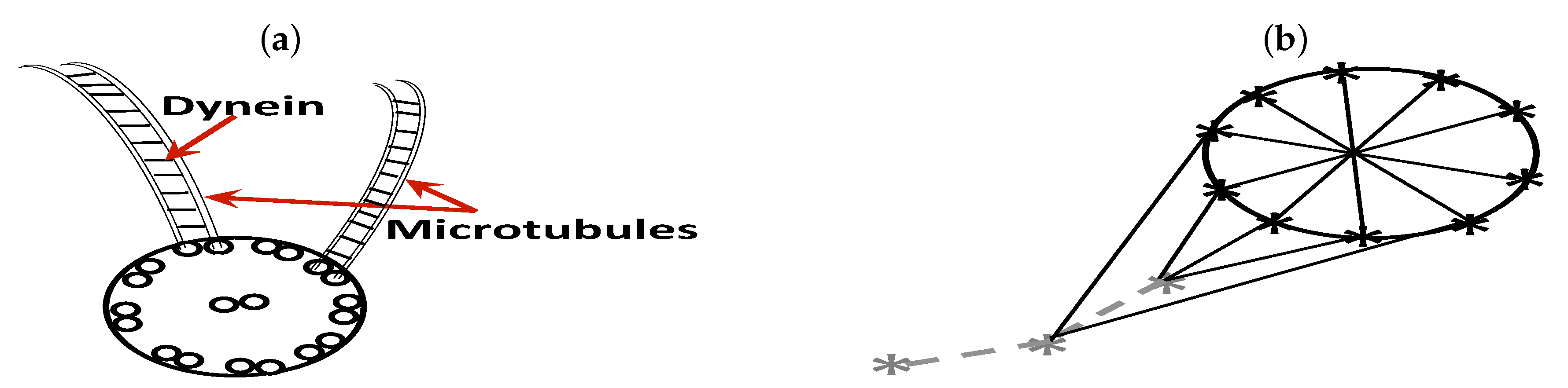
2.2. Sperm Representation

Based on previous recordings of the flagellar beat form of human sperm [39], we assume that the swimmer will propagate a curvature wave along the tail, with larger magnitude at the end of the tail (furthest away from the head). The preferred tail beat form of the q-th swimmer is given by:

$${\overline{\mathbf{X}}}_T^q(s,t)=[\overline{x}(s,t),\overline{y}(s,t)]=[s,\beta (1-s)sin(\kappa s-\sigma t)],$$

where t is time and s is an arc length parameter, $0\le s\le L$ for tail length L with $s=0$ the end of the tail and $s=1$ closest to the cell body. The bar will denote any quantity that corresponds to the preferred configuration. As summarized in

Table 1. Baseline parameters for swimmer model.

$\mathcal{T}$, characteristic time scale,	0.05 s (beat frequency 20 Hz)
$\mathcal{L}$, characteristic length scale	50 $\mathsf{\mu }$m
$\mathcal{V}$, characteristic velocity scale	$\mathcal{L}/\mathcal{T}$ (wavespeed)
$\mu$, viscosity	0.001 kg m${}^{-1}$ s${}^{-1}$
$\mathcal{F}$, characteristic force scale	$\mu \mathcal{V}\mathcal{L}$
L, tail length	1
$r_h$, head radius	0.1
$\kappa$, wavenumber	$2\pi$
$\beta$, amplitude	varied [0.1,0.3]
$\sigma$, frequency	$4\pi$
$S_C$, curvature stiffness of tail	8
$S_T$, tensile stiffness of tail	10,000
$S_N$, tensile stiffness of neck	500
$S_H$, tensile stiffness of head	10,000
$S_{H,C}$, curvature stiffness of head	0.8
$S_{N,A}$, stiffness for tail-head connecting angle	10,000

, the preferred non-dimensional beat form parameters are: amplitude $\beta$, beat frequency $\sigma /2\pi$, and wavelength $2\pi /\kappa$. The relative scales of these parameters are based on those of human sperm [39].

We will assume that the tail can be modeled as an Euler elastica. Hence, elastic energies corresponding to active bending and passive tension can be determined and will tend to be minimized when the preferred beat form is achieved [29,30,40]. Let ${\mathsf{\Omega }}_T^q$ correspond to the tail of the q-th swimmer, and let the actual and preferred curvature of the tail, ${\mathsf{\Lambda }}^q$ and $\overline{\mathsf{\Lambda }}(s,t)$, be given as

$${\mathsf{\Lambda }}^q(s,t)=\frac{\frac{{\partial }^2{y}^q}{\partial s^2}\frac{\partial x^q}{\partial s}-\frac{{\partial }^2{x}^q}{\partial s^2}\frac{\partial y^q}{\partial s}}{{\left({\left(\frac{\partial x^q}{\partial s}\right)}^2+{\left(\frac{\partial y^q}{\partial s}\right)}^2\right)}^{3/2}},\overline{\mathsf{\Lambda }}=\frac{{\partial }^2\overline{y}}{\partial s^2},$$

(3)

where ${\mathit{X}}_T^q=[x^q,y^q]$ is the actual tail location at time t. The energy corresponding to the dynein motors generating a curvature wave on the tail is given as

$${\mathcal{E}}_C^q=S_C{\int }_{{\mathsf{\Omega }}_T^q}{\left({\mathsf{\Lambda }}^q(s,t)-\overline{\mathsf{\Lambda }}(s,t)\right)}^{2}ds.$$

(4)

The stiffness coefficient $S_C$ determines how strictly the preferred configuration is enforced. The tension component of the tail energy, ${\mathcal{E}}_T$, is an effective inextensibility constraint and is given as

$${\mathcal{E}}_T^q=S_T{\int }_{{\mathsf{\Omega }}_T^q}{\left(\left|\left|\frac{{\partial }^2{\mathit{X}}_T^q}{\partial s^2}\right|\right|-1\right)}^{2}ds.$$

(5)

Here, the stiffness coefficient $S_T$ captures the rigidity of the microtubules in the tail and their resistance to bending (refer to Figure 1a). We note that $S_T$ and $S_C$ have been previously calibrated for this model to be in the range of mammalian sperm [19].

We assume that the cell body is circular with radius $r_h$ (preferred curvature $\overline{\eta }=1/r_h$), with the circle denoted by ${\mathsf{\Omega }}_H^q$. Since the cell body is a passive and rigid structure attached to the filament, we will also utilize a head curvature energy ${\mathcal{E}}_{H,C}$:

$${\mathcal{E}}_{H,C}^q=S_{H,C}{\int }_{{\mathsf{\Omega }}_H^q}{\left({\eta }^q(s,t)-\overline{\eta }(s,t)\right)}^{2}ds.$$

The actual head curvature ${\eta }^q$ for the q-th swimmer is calculated in the same way as ${\mathsf{\Lambda }}^q$ in Equation (3), with the caveat that curvature is now calculated using the current head location ${\mathit{X}}_H^q=[x^q,y^q]$. An effective inextensibility constraint is also utilized for the head, similar to Equation (5). As shown in Figure 1b, this constraint is comparable to Hookean springs connecting all discretization points on the perimeter of the head as well as connecting points on the circular head that are $\pi$ apart. In order for the head to be passively pushed by the active tail, we also have a series of stiff connections between the head and the flagellum in the neck region (refer to Figure 1b). Five springs are utilized to connect the first two points on the flagellum (right-most) to the head, all with stiffness coefficient $S_N$. The corresponding energy will be similar to Equation (5). In addition, an additional energy that penalizes deviations from the initialized vector between the point on the tail at $s=1$ and the midpoint of the cell body is enforced with a stiffness coefficient $S_{N,A}$ [41].

2.3. Numerical Methods

For all numerical simulations, the time step is $▵t=$10${}^{-5}$. The swimmer is always initialized as a straight line, and has $N_T=100$ points on the tail when $L=1$. Tail points are increased with the same discretization spacing for $L>1$. Similarly, $N_H=48$ is the number of points on the head when the head radius is $r_h=0.1$ and head points are increased (or decreased) to maintain a constant head discretization spacing when $r_h\ne 0.1$.

In order to solve for the resulting fluid flow $\mathit{u}$ in Equation (1), we will first have to determine the forces $\mathbf{f}$. The point forces ${\mathbf{F}}^q$ that the q-th swimmer exerts on the surrounding fluid can be obtained by a variational derivative of the total energy [41,42],

$$\begin{array}{cc}\hfill {\mathit{F}}^q& =-\frac{\partial {\mathcal{E}}^q}{\partial {\mathit{X}}^q}\hfill \\ \hfill & =-\frac{\partial }{\partial {\mathit{X}}^q}\left({\mathcal{E}}_C^q\left({\mathit{X}}_T^q\right)+{\mathcal{E}}_T^q\left({\mathit{X}}_T^q\right)+{\mathcal{E}}_{H,C}^q\left({\mathit{X}}_H^q\right)+{\mathcal{E}}_{H,T}^q\left({\mathit{X}}_H^q\right)+{\mathcal{E}}_N^q({\mathit{X}}_T^q,{\mathit{X}}_H^q)\right).\hfill \end{array}$$

(6)

The terms on the right hand side of Equation (6) are: tail curvature energy ${\mathcal{E}}_C$, tail tensile energy ${\mathcal{E}}_T$, head curvature energy ${\mathcal{E}}_{H,C}$, head tensile energy ${\mathcal{E}}_{H,T}$, and neck junction energy ${\mathcal{E}}_N$. Discretizing the energy integrals and taking derivatives leads to a singular force layer, which we regularize to obtain $\mathit{f}=\mathit{F}{\varphi }_{ϵ}\left(r\right)$. Here, ${\varphi }_{ϵ}\left(r\right)$ is a radially symmetric blob function that satisfies ${\int }_0^{\infty }r{\varphi }_{\delta }dr=\frac{1}{2\pi }$ [43]. For a point ${\mathit{X}}_i$ on the swimmer, $r=|\mathit{x}-{\mathit{X}}_i|$ and we choose

$${\varphi }_{ϵ}\left(r\right)=\frac{3{\delta }^3}{2\pi {(r^2+{\delta }^2)}^{5/2}},$$

(7)

fixing the regularization parameter as $ϵ=0.02$ for all simulations [29,30]. After regularizing the forces, we can write the solution to the velocity $\mathit{u}$ as a superposition of all of the point forces. This is the method of regularized Brinkmanlets and as detailed in [30,31] for a 2-d fluid,

$$\begin{array}{cc}\hfill \mathrm{p}\left(\mathit{x}\right)& =\sum _{q=1}^M\sum _{i=1}^N{\mathit{F}}_i^q\nabla G_{ϵ}\left(r\right),\hfill \end{array}$$

(8)

$$\begin{array}{cc}\hfill \mathit{u}\left(\mathit{x}\right)& =\sum _{q=1}^M\sum _{i=1}^N\left[-{\mathit{F}}_i^q(B_{ϵ}^{″}\left(r\right)+c_{\alpha }+c_S)+({\mathit{F}}_i^q·(\mathit{x}-{\mathit{X}}_i))(\mathit{x}-{\mathit{X}}_i)\frac{r{B}_{\delta }^{″}\left(r\right)-B_{\delta }^{\prime }\left(r\right)}{r^3}\right],\hfill \end{array}$$

(9)

where $r=|\mathit{x}-{\mathit{X}}_i^q|$, ${\varphi }_{ϵ}={\nabla }^2{G}_{ϵ}$, and $B_{ϵ}$ is implicitly defined as $(\mathsf{\Delta }-{\alpha }^2)B_{ϵ}=G_{ϵ}$ for radially symmetric $G_{ϵ}$ and $B_{ϵ}$. The other terms in Equation (9) are

$$c_{\alpha }=\frac{-{\gamma }_e-log(\alpha /2)}{4\pi },c_S=-\frac{{\mathit{F}}_i^q}{8\pi },$$

where ${\gamma }_e$ is the Euler-Mascheroni constant and these terms are derived to ensure that as $\alpha \to 0$, we recover the singular Stokeslet where the remaining constant flow is canceled out with $c_S$. Here, the total number of swimmers and points on each swimmer is M and $N=N_T+N_H$, respectively. Details of the numerical method are given in Leiderman et al. [30,44]. The main numerical algorithm involves solving for the forces that the swimmer exerts on the fluid at each time instant, then evaluating the instantaneous fluid velocity, and then updating the swimmer using a no-slip condition, $d{\mathit{X}}^q/dt=\mathit{u}\left({\mathit{X}}^q\right)$. This enforces that the swimmer moves at the local fluid velocity.

3. Results

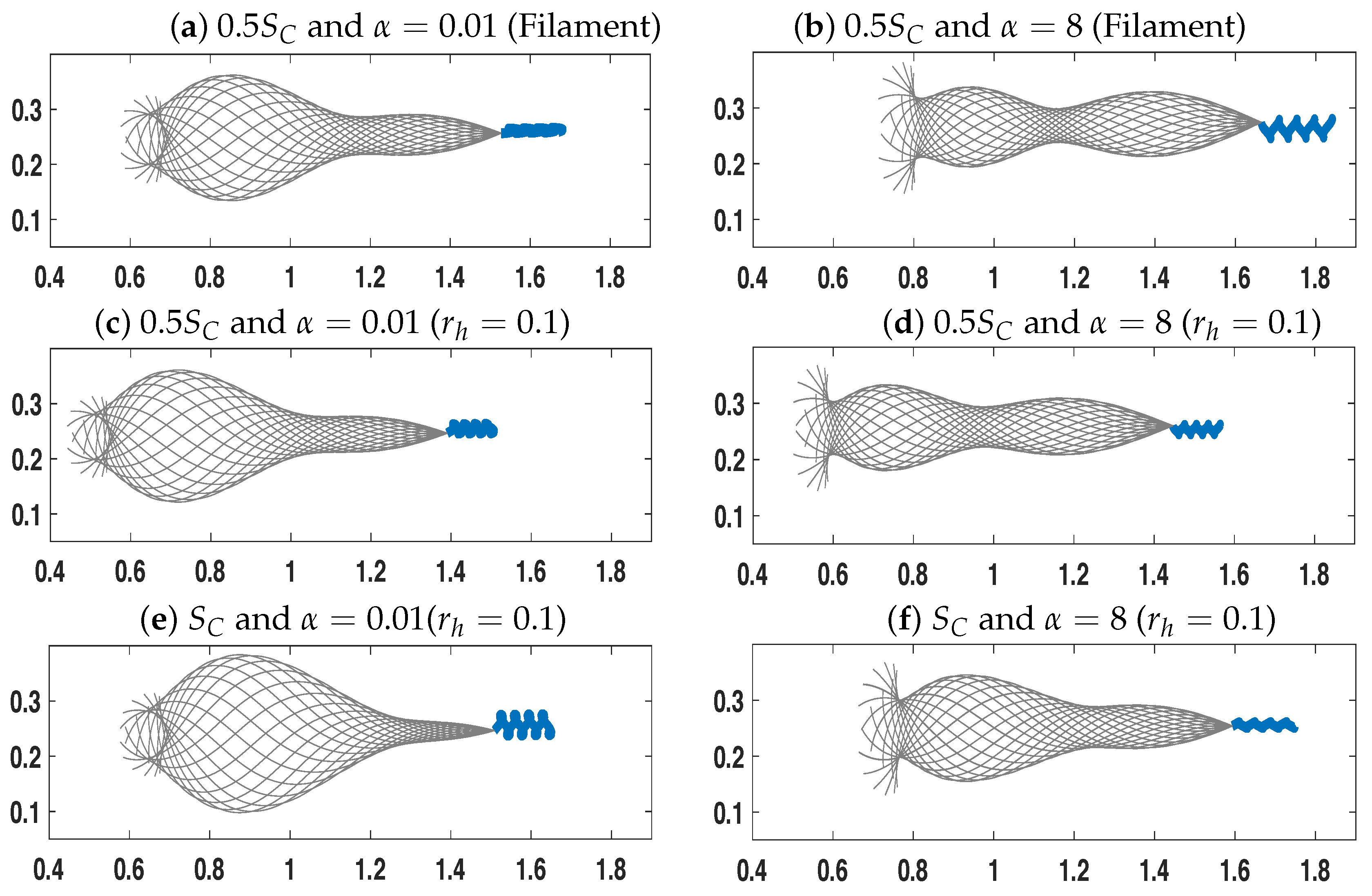
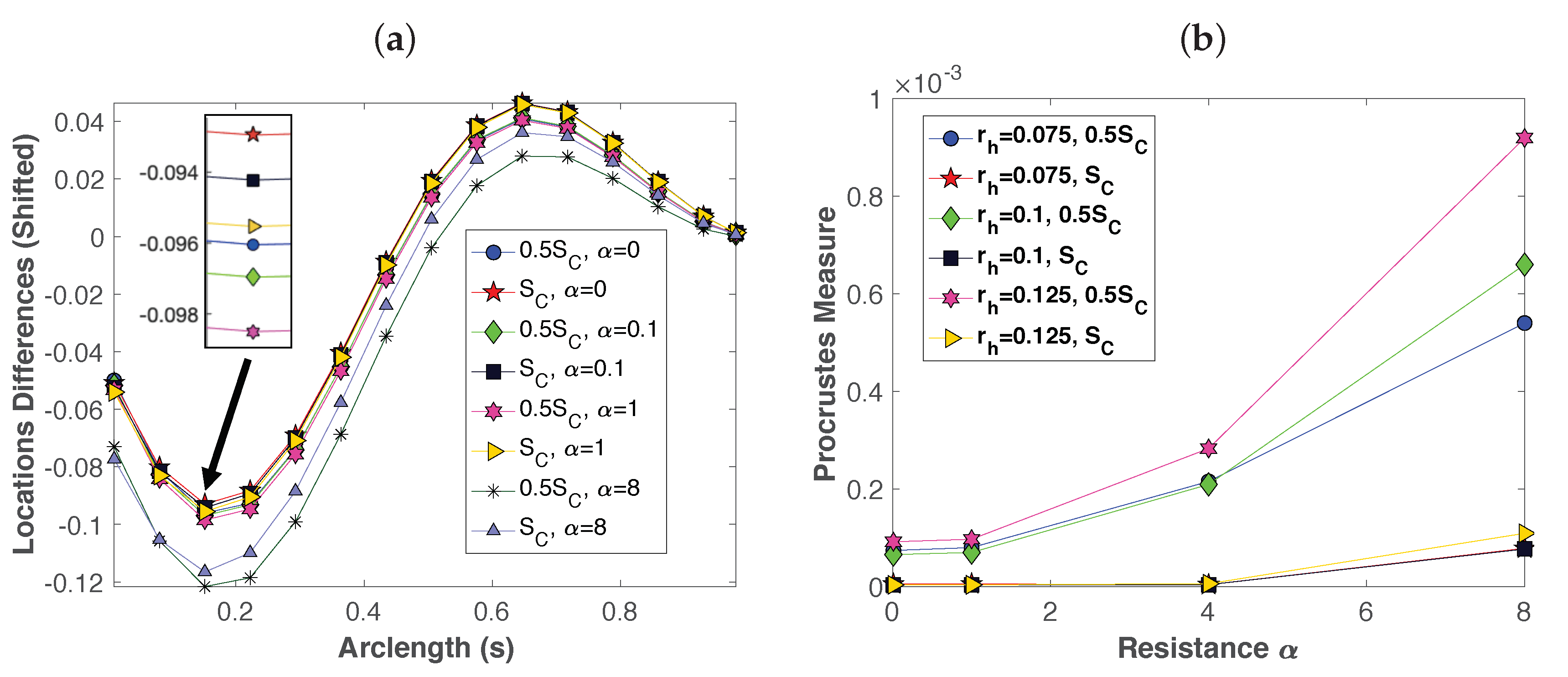
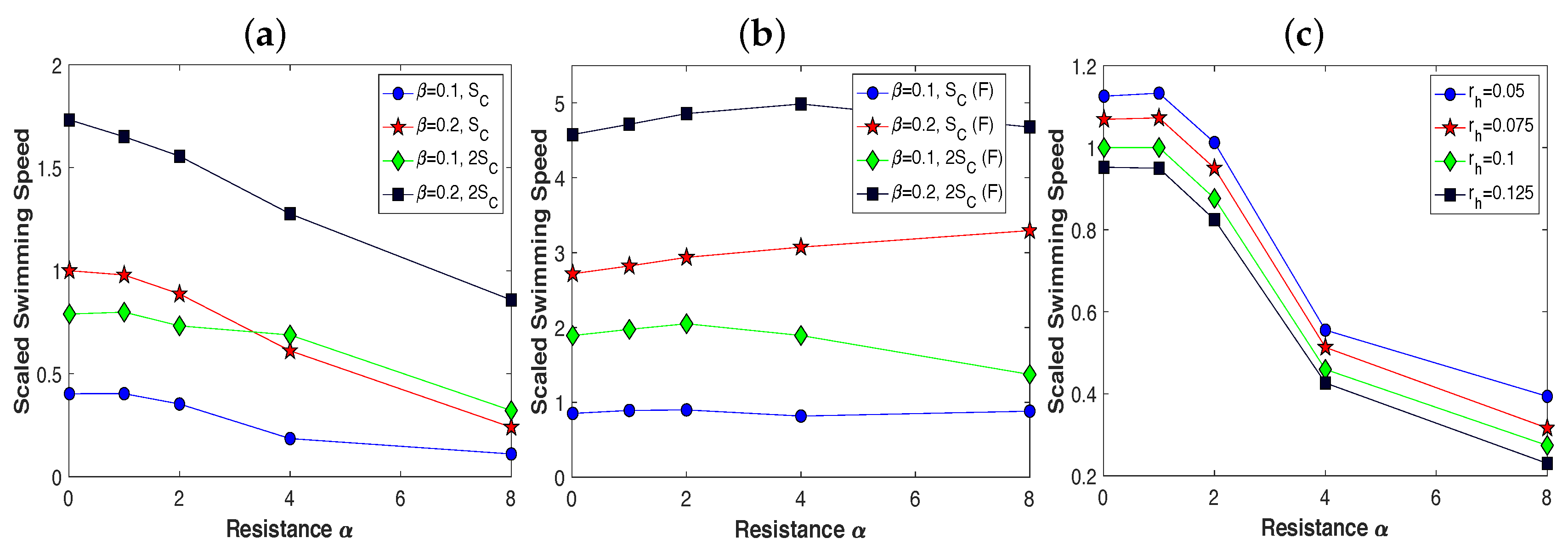
3.1. Dynamics of a Single Swimmer

We were first interested in understanding how model parameters could lead to different emergent beat forms and swimming speeds. In Figure 2, traces of the cell body and overlayed tail positions are shown over four beat periods (from non-dimensional time $t=8-10$). We emphasize that the x-axes of each graph are constant and all swimmers are initialized at the same initial location with the same exact preferred beat form. The energy in Equation (4) specifies the preferred curvature but due to resistance in the fluid and material parameters (corresponding stiffness coefficients) of the swimmer, the emergent tail positions minimize this energy. In comparing the case of $\alpha =0.01$ in Figure 2a,c,e and $\alpha =8$ in Figure 2b,d,f, we observe the preferred taper of the tail from the head to the end of the tail for $\alpha =0.01$ (very small volume fraction of fibers). In comparison, $\alpha =8$ does not achieve the preferred taper; this is due to the larger resistance in the fluid on this cell body. For these baseline parameters in Figure 2, we also explored emergent beat forms as the stiffness $S_C$ is varied, which enforces how closely the preferred curvature is followed. Figure 2c,d, the second row, has $S_C$ as half the baseline amount and has the baseline value in Figure 2e,f, the bottom row; for each case of $\alpha$, $0.5S_C$ deviates more from the preferred configuration.

Previous models have been of a filament (no head or $r_h=0$); we observe that the filament in Figure 2a,b swims faster than the swimmer with head radius $r_h=0.1$ in Figure 2c,d for the same parameters. Even though increased progression is made in the case of the filament, the emergent beat form is similar. We further explore emergent beat forms in Figure 3. At $t=15$ non-dimensional time, the differences between the preferred and emergent beat form are given in Figure 3a, where x-locations are shifted to have swimmer configurations overlayed. We observe larger differences at the end of the tail in comparison to closer to the cell body. This is due to the rigid springs that are connecting the head and the flagellum, as shown in Figure 1b. The deviations from the preferred beat form increase as resistance parameter $\alpha$ is increased, and increase as the curvature stiffness $S_C$ is decreased. To further compare the differences in beat forms with and without a cell body or head, we utilized the Procrustes Measure. This measure is a sum of squared errors that gives the dissimilarity between the filament (no head or $r_h=0$) beat form and the corresponding simulation with head radius $r_h\ne 0$. The measure is calculated after the beat forms of the case of a head has been translated and rotated to coincide with the filament case. The metric is very small because all emergent beat forms are still represented by a tapered sine wave. However, the metric highlights that at smaller curvature stiffness, $0.5S_C$, the beat forms of swimmers with a head are more dissimilar to the filament as resistance parameter $\alpha$ increases and as head radius $r_h$ increases.

Since the swimmer is moving with the local flow field, we further investigate this in Figure 4. Flow fields and the corresponding pressure are shown for six different sets of parameters after 30 beat periods of the tail. We observe local vortices around the tail where the motion of the tail coincides with the fluid. Additionally, as the tail is pushing on the surrounding fluid, we observe corresponding peaks in the pressure. Since the fluid computations are for an infinite fluid in 2-d, the flow and pressure are lower in magnitude away from the swimmer. The tail trajectory is shown with the gray curve and the axes of each graph are constant. In each of these plots, the swimmer is initialized at the same initial location and are given the same exact preferred beat form. In the top row of Figure 4a,b, this is the case of preferred beat amplitude $\beta =0.2$ and we observe increased forward progress in comparison to the second row of Figure 4c,d with amplitude $\beta =0.1$ (with all other parameters the same). In comparing the tail traces between the left column with $\alpha =0.01$ and the right column with $\alpha =8$ in Figure 4, similar to Figure 2, we observe a smaller amplitude at the end of the tail for the smaller resistance parameter. In Figure 4e,f, the bottom row, the head radius is decreased by half and as a result, we observe decreased pressure directly behind the head (in comparison to the top two rows in Figure 4).

Often times we are interested in the swimmer and/or fluid properties that allow for the greatest forward progression, since this will correlate with the ability of the sperm to reach and fertilize the egg [3,5]. In Figure 5, all swimming speeds are scaled by the baseline case of head radius $r_h=0.1$, $\alpha =0.01$, $\beta =0.2$, and curvature stiffness $S_C$ from Table 1. In Figure 5a, due to this scaling, the swimming speed starts at 1 for these parameters and then decreases as $\alpha$ increases. This trend is the same for the other cases of $S_C$ and $\beta$; in this parameter regime, obstructions in the fluid cause swimming speeds to decrease. For a fixed $\beta$, as shown in Figure 5a, the swimming speed increases for larger curvature stiffness $S_C$. Similarly, for fixed curvature stiffness, swimming speed is larger for larger preferred amplitude $\beta$. Comparing a swimmer with a head radius $r_h=0.1$ to the case of a filament ($r_h=0$), we observe an increased swimming speed for the filament in Figure 5b. For the baseline case of $\beta =0.2$ and $S_C$, the filament is around 2.8 times faster than the swimmer with head radius $r_h=0.1$. This increased swimming speed of the filament relative to the swimmer with a head is consistent for the range of $\alpha$ studied. In Figure 5b, for a filament (no head or head radius $r_h=0$), we observe that doubling amplitude $\beta$ results in a significant increase in swimming speed. The swimming speeds decreased in Figure 5a as $\alpha$ increased, but for the filament in Figure 5b, there was a non-monotonic change in swimming speed as $\alpha$ increased. As shown in Figure 2, Figure 3 and Figure 4, the emergent beat form changes and this complex relationship between emergent beat form parameters and fluid properties determines the amount of forward progression. Figure 5c also shows that due to increased drag on the head, as the head radius is increased, the swimmer decreases forward progression, regardless of resistance parameter $\alpha$.

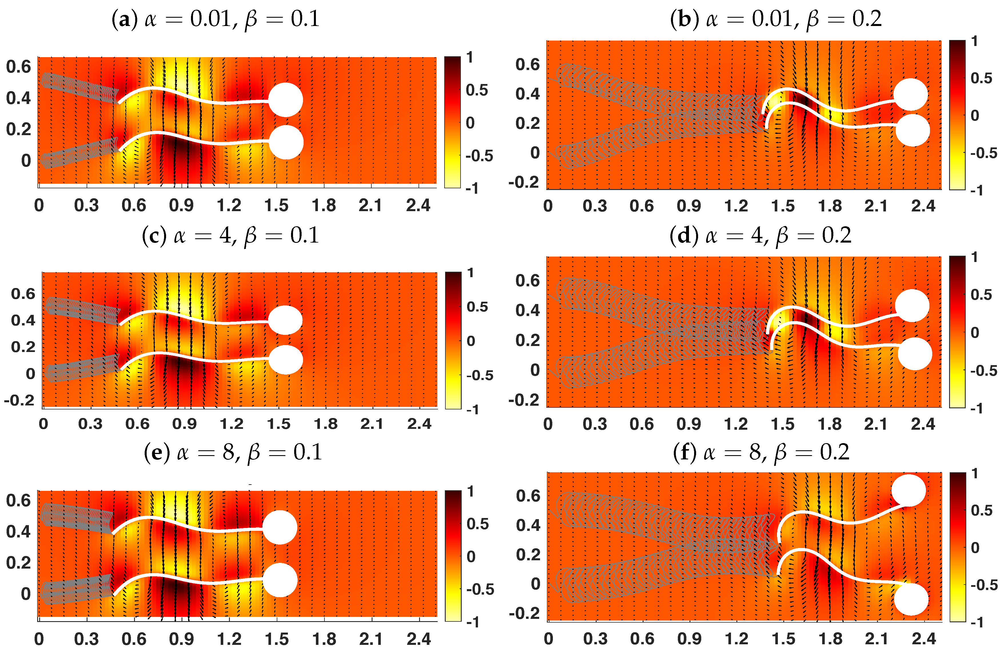
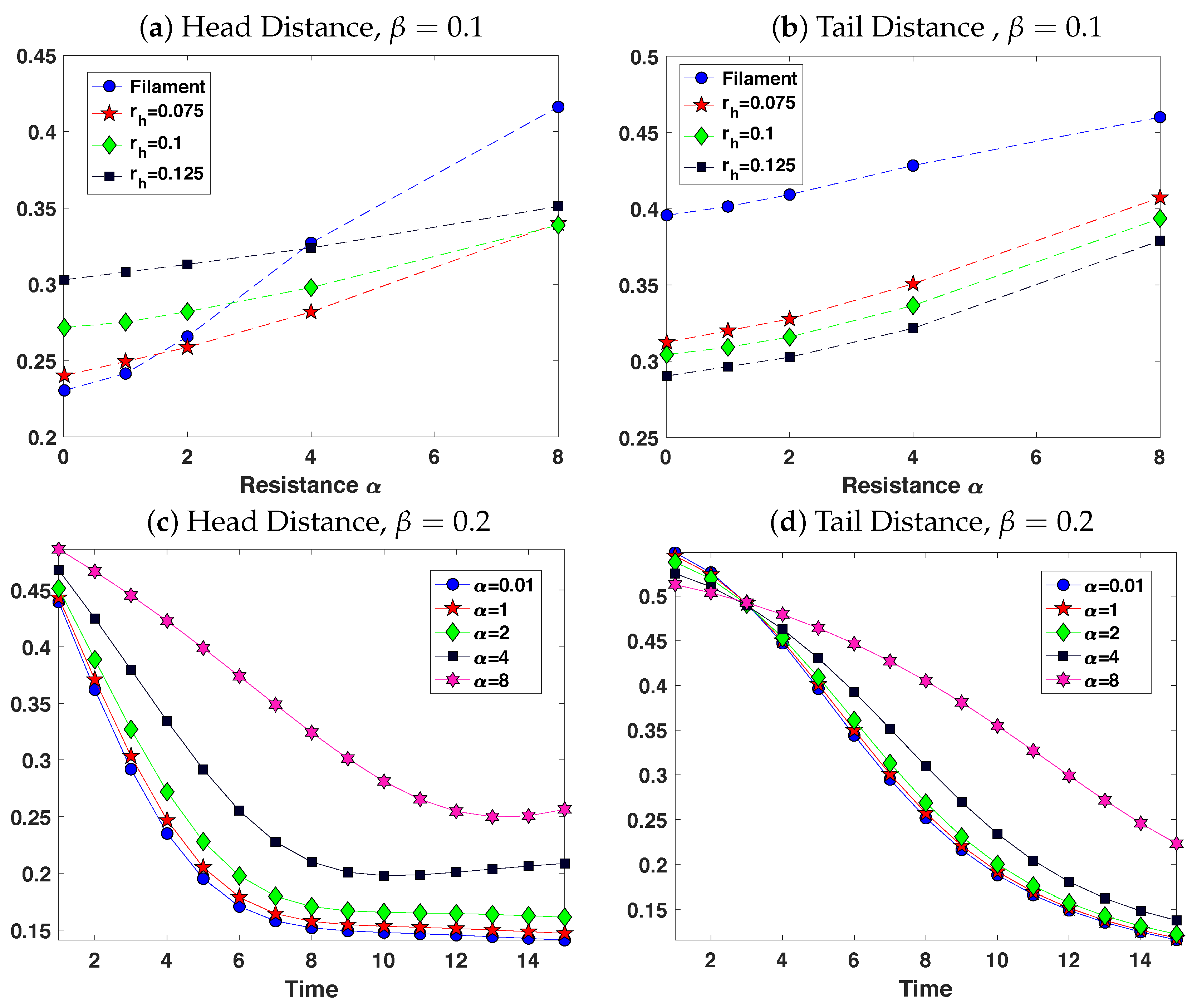
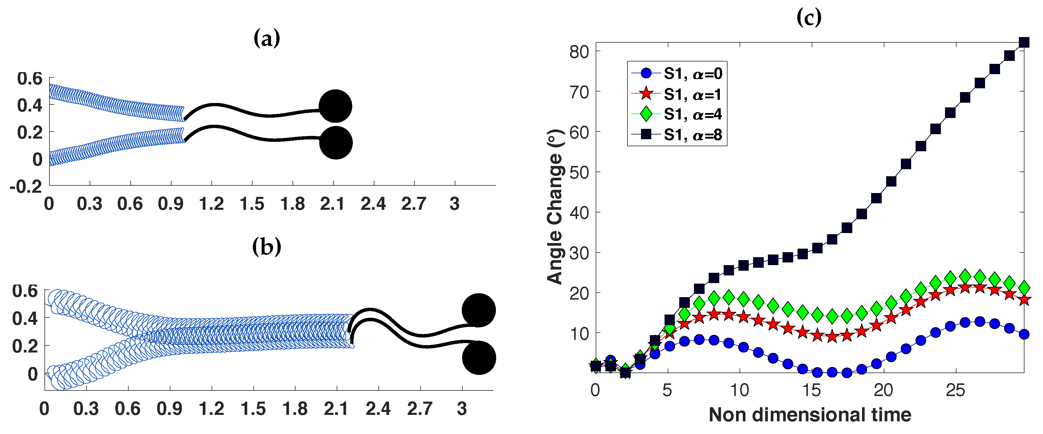
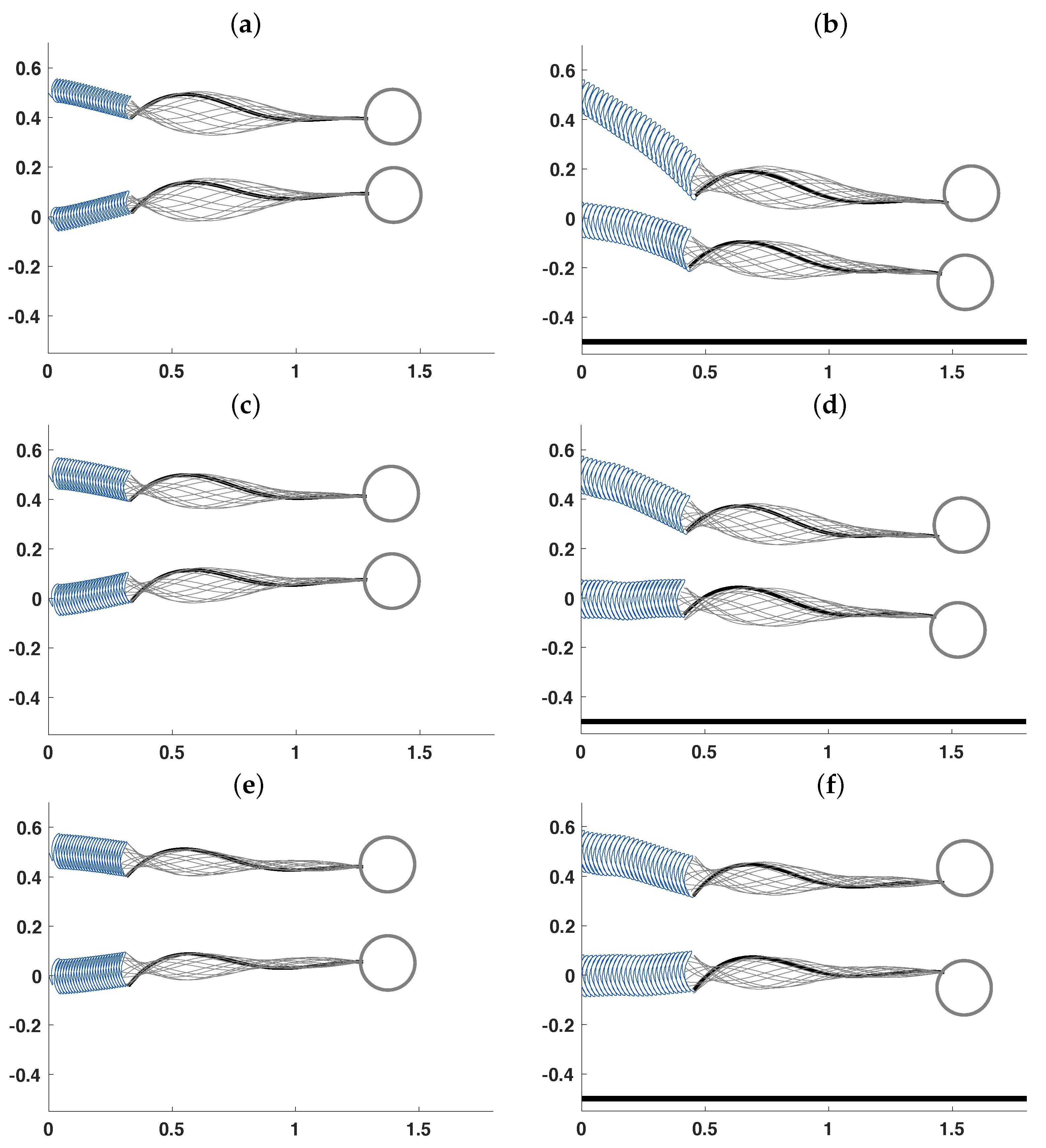
3.2. Pairs of Swimmers

In the above section, we have observed that as expected, the size of the cell body or head geometry, as well as the resistance parameter will change the swimming dynamics. As has been previously reported both in experiments and model simulations, pairs of swimmers will tend to attract and synchronize their flagellar beat [8,30,40,45]. This was the case of filaments in a Stokesian and Brinkman fluid where enhanced swimming speed (in comparison to a single swimmer) was observed when filaments attracted and synchronized. In the case of a Brinkman fluid, attraction was observed when the pairs of swimmers (filaments without a head) were less than $1/\alpha$ apart, which corresponded to the Brinkman screening length [30,34]. The question that is now being investigated is how or whether attraction will occur between swimmers in a Brinkman fluid when the cell body is accounted for. The setup is the same as for a single swimmer except that each swimmer feels the other swimmer through the surrounding fluid. Additionally, when swimmers (points on the head or tail of different swimmers) are within 4$ϵ$ of each other, we utilize an additional repulsive force to ensure that structures do not cross into each other. Similar to the discretization on the tail for the tension forces, it acts as a Hookean spring with stiffness $S_R=0.05$ [40]. The distance between every point on the swimmers is calculated and this force only turns on at the sub-set of points that are less than 4$ϵ$ apart (zero for the majority of the time points in the simulation).

In Figure 6, we initialize swimmers a vertical distance of $I_d$ apart and at the same starting location with the same preferred curvature, and show the flow field and pressure after 30 beat periods (non-dimensional time $t=15$). Similar to Figure 4, the trace of the last point of the tail is shown for each swimmer and we observe a decrease in vertical distance between the tails for all plots in Figure 6. Figure 6a,c,e, the left column, is for smaller amplitude $\beta =0.1$ and Figure 6b,d,f, the right column, is for larger amplitude $\beta =0.2$. In the 30 beat periods, the larger resistance parameter $\alpha$ in Figure 6e attracts less than in Figure 6a,c. The increased resistance and hence, volume fraction of fibers, is preventing the swimmers from attracting on a fast time scale in Figure 6e. The larger amplitude in the right column allows for additional forward progression and greater attraction in the vertical direction. For the lower resistance parameter $\alpha$ in Figure 6b,d, there is stable attraction over the time period. In contrast, even though $\alpha =8$ in Figure 6f, the larger amplitude generates additional propulsive thrust and can push the fluid out of the way in order for the swimmers to attract initially. However, due to the large drag on the cell body, the beating tails at later time points cause the cell body to rotate slightly, causing the sperm to separate.

The dynamics of attraction for this same pair of swimmers is further explored in Figure 7. At non-dimensional time $t=15$, the distance between the centers of the head (or the first point on the swimmer in the direction of swimming for the case of a filament) is shown for preferred amplitude $\beta =0.1$ in Figure 7a. Interestingly, the filament (no head, F) is able to get the closest by $t=15$ (30 beat periods) for $\alpha =0$ and 1 whereas the distance between the tails is larger as shown in Figure 7b. In addition, whereas the filament (no head, F) stays further apart at $\alpha =8$ in Figure 7a,b in terms of head and tail distance, respectively, the swimmers with heads are able to attract more closely. The case of larger amplitude is shown in Figure 7c,d over the time interval $t=0-15$ for the head and tail distances, respectively. As observed in the right column of Figure 6, the larger amplitude allows the swimmers to experience increased attraction, especially for lower to moderate resistance parameter $\alpha$. For larger $\alpha$, the head reaches maximal attraction around $t=12$ or 24 beat periods and then starts to slowly push apart whereas the end of the tail continues to attract and beat in synchrony.

There are many questions about whether swimming in pairs or groups can be more efficient, potentially giving an increase in the collective swimming speed. Previous work has shown increases in swimming speeds in a Stokesian fluid [40] for a pair of finite-length filaments. In Figure 8a, average progressive velocity for the pair of filaments (no head) in a Brinkman fluid is shown, scaled by the speed of the corresponding solo filament simulation with the same parameters. The swimming speed of a pair of swimmers in Figure 8a is slower (scaled speed always $<1$) than the corresponding solo swimmer for larger resistance $\alpha$ when initialized $I_d=0.5$ or 2.0 apart. In stark contrast, the pair of swimmers with head radius $r_h=0.1$ in Figure 8b swims faster (scaled speed $>1$) than the corresponding solo swimmer for larger resistance $\alpha$ ($\alpha \ge 4$) when initialized $I_d=0.5$ apart. This is contrary to intuition since swimming speed and attraction is enhanced with a small volume fraction of fibers in the fluid. In comparison, when $I_d=2$ in Figure 8b, there is a small decrease in swimming speed for most of the resistance parameter values examined.

We further explore the potential stability of this attraction by running simulations out to $t=30$. Trajectories for resistance parameter $\alpha =0$ with preferred amplitude $\beta =0.1$ are in Figure 9a whereas Figure 9b is for $\beta =0.2$. The swimmers continue to attract in Figure 9a and remain stably attracted over this additional time period in Figure 9b. However, there is a question of whether these two swimmers will eventually push apart, especially in the case of Figure 9b where it looks like the head of the upper swimmer is moving upward. To investigate the trajectories of these pairs of swimmers, we characterized the direction of swimming as the vector connecting the center of mass of the tail and the center of the head, either $\overrightarrow{S1}$ for the top swimmer or $\overrightarrow{S2}$ for the bottom swimmer. Angle changes or deviations from the trajectory of a solo swimmer (direction given by $\overrightarrow{Solo}$) is calculated as:

$$\theta =arccos\left(\frac{\overrightarrow{S1}·\overrightarrow{Solo}}{|\overrightarrow{S1}\left|\right|\overrightarrow{Solo}|}\right),$$

(10)

where the numerator is the dot product of the vectors and the denominator has the standard Euclidean norm for each vector. Note that we are just calculating the the angle between the solo swimmer and one of the two swimmers; we do not capture whether this angle is causing the swimmer to push down or move up, but this can be gathered from previous figures. In Figure 9c, for $\beta =0.2$, we show the angle differences for the top swimmer S1 (similar patterns are observed for S2). For $\alpha =8$, this angle difference continues to increase in time; the top swimmer continues to swim further up and away from the trajectory of the solo swimmer. From Figure 6f, we classified the swimmers as starting to push apart at $t=15$, corresponding to an angle difference of $\theta ={30}^{\circ }$ (shown in Figure 9c). In the case of $\alpha =0$, Figure 9c shows that angle changes are much smaller but they are oscillating and growing in time (small rate of growth). For $\alpha =1$ and $\alpha =4$, the oscillations and continued growth are also present. Based on these angle changes that continue to slowly grow, we predict that attraction will be stable for a long period of time, but that when $\theta \ge {30}^{\circ }$, this would then change from attracted swimmers to those that are starting to push away.

The presence of a head, and its size, also changes the dynamics of attraction.

Table 2. Angle differences at $t=15$, calculated using Equation (10). $S1$ and $S2$ correspond to the top and bottom swimmers, respectively, when centerlines are initialized a distance $I_d=0.5$ apart. F corresponds to filament (no head).

Parameters	$\mathit{\alpha }=0$	$\mathit{\alpha }=1$	$\mathit{\alpha }=4$	$\mathit{\alpha }=8$
S1, $\beta =0.1$, $r_h=0.1$	4.1427	4.0591	3.3784	2.6849
S2, $\beta =0.1$, $r_h=0.1$	2.6702	2.5901	2.1684	1.4504
S1, $\beta =0.2$, $r_h=0.1$	29.8417	10.0230	12.0022	21.1165
S2, $\beta =0.2$, $r_h=0.1$	2.7297	3.1615	6.3438	15.9360
S1, $\beta =0.1$, $r_h=0$ (F)	8.5972	8.3903	6.1374	3.4372
S2, $\beta =0.1$, $r_h=0$ (F)	0.7264	0.7264	0.4022	1.0445
S1, $\beta =0.2$, $r_h=0$ (F)	5.3680	5.3680	6.1029	3.6030
S2, $\beta =0.2$, $r_h=0$ (F)	1.5309	1.2868	0.7523	0.3240

delineates the deviations in the angle, in comparison to the solo swimmer, at $t=15$ for a variety of cases. In general, we note that the top swimmer S1 generally has a slightly larger change in angle than the bottom swimmer S2 for the smaller amplitude case, $\beta =0.1$, for both head radius $r_h=0.1$ and the filament ($r_h=0$). In addition, the angle changes at $t=15$ in the direction of swimming are non-monotonic with respect to resistance parameter $\alpha$ for $\beta =0.2$ for the bottom swimmer S2. At smaller amplitudes, angle changes decrease with respect to increasing $\alpha$ for the top swimmer S1.

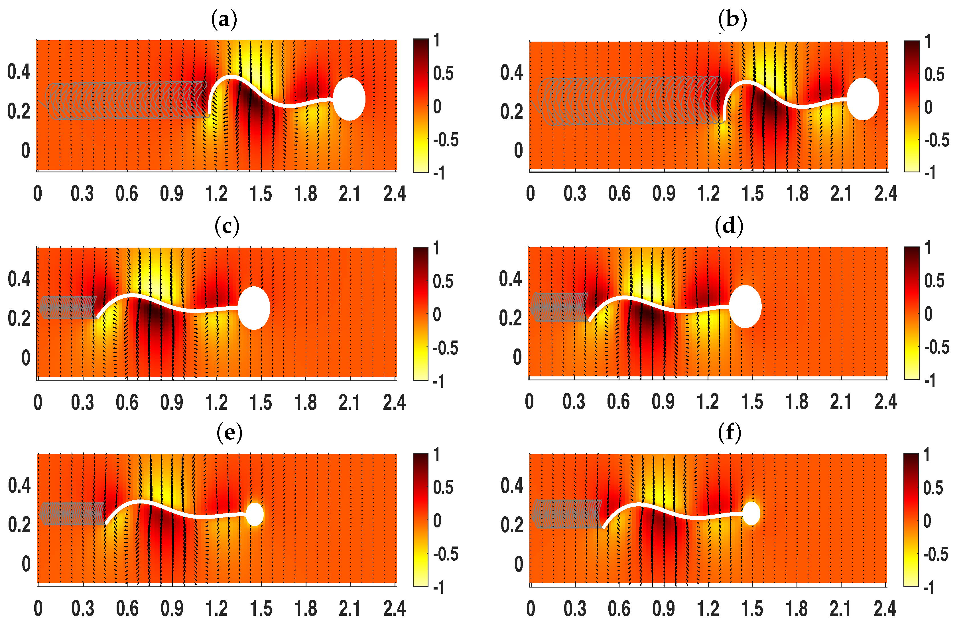
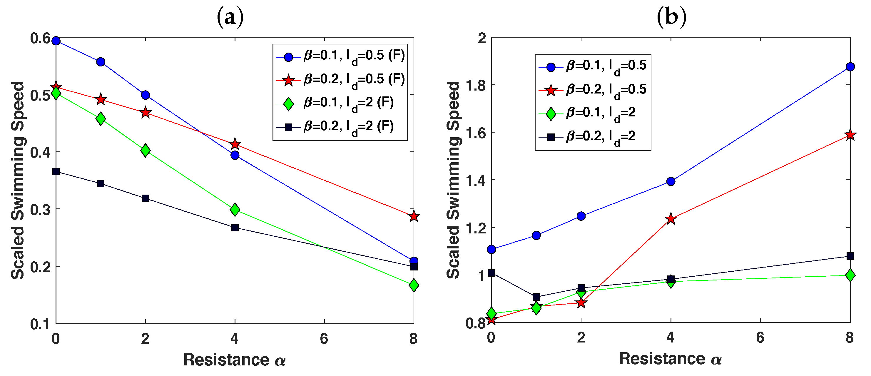
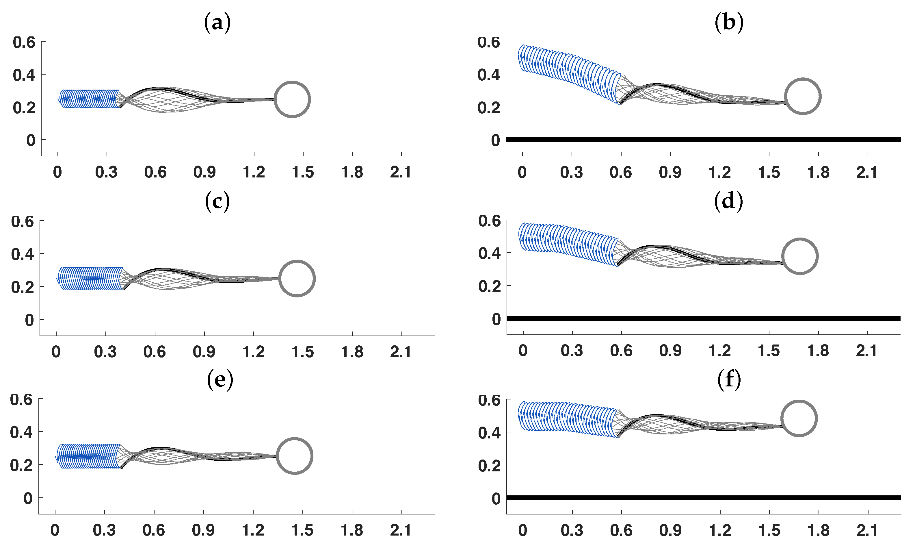
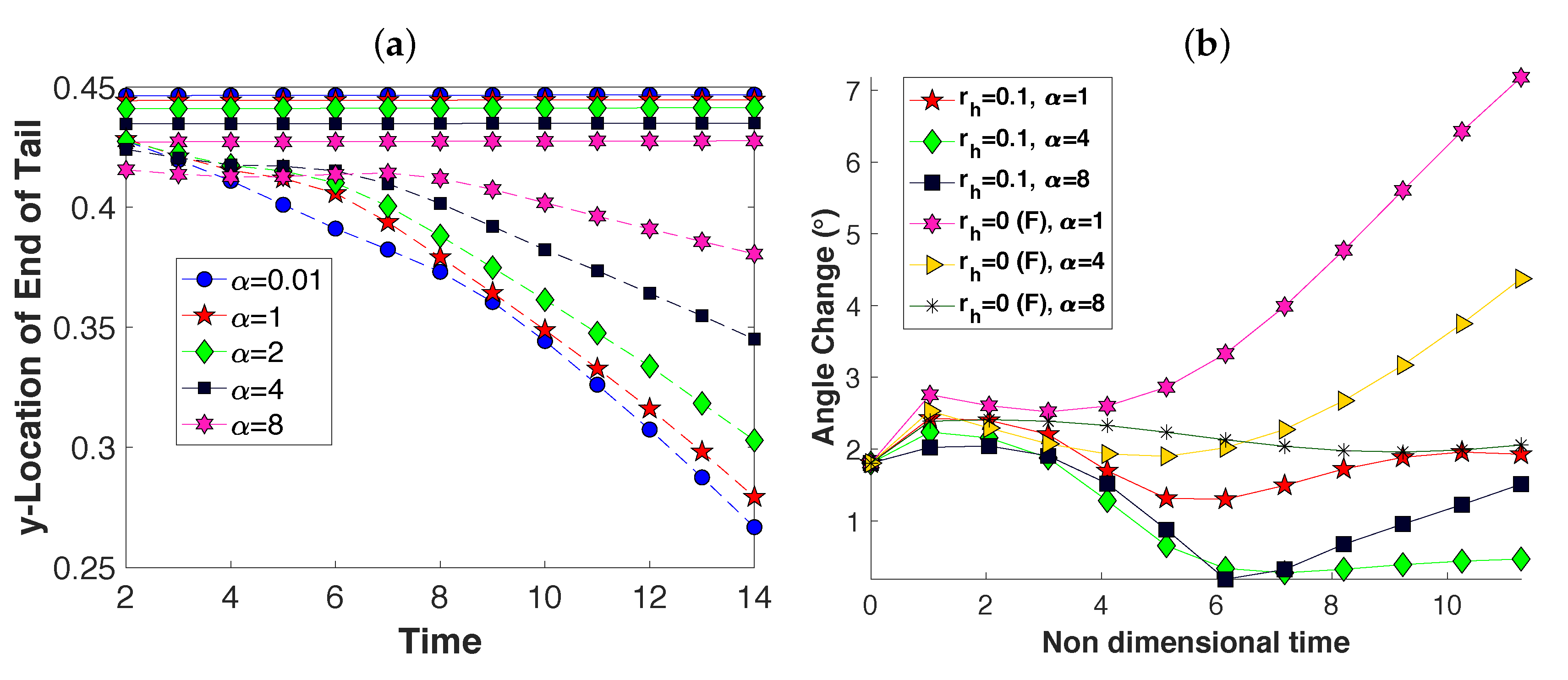
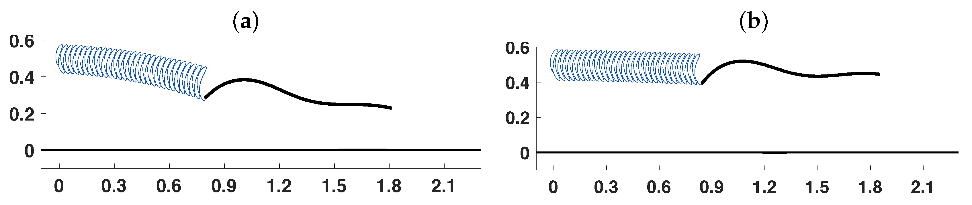
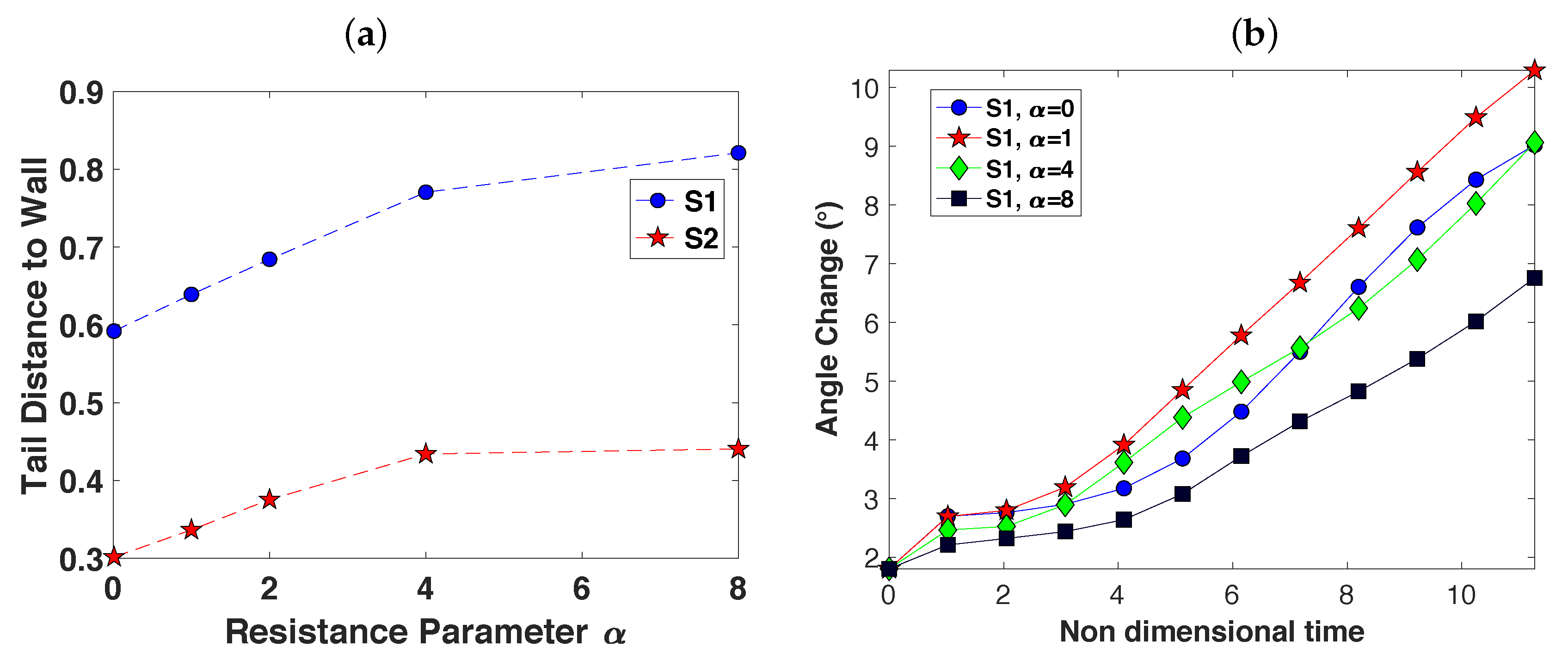
3.3. Wall Interactions

Sperm must navigate complex environments, interacting with boundaries such as the oviductal epithelium in order to reach and fertilize the egg [5]. We explore wall interactions of a swimmer by modeling the wall as an elastic boundary, which will be composed of energy functionals similar to those in Equations (4) and (5), where we assume that the wall will have a preferred curvature of zero and we want to maintain an effective inextensibility constraint. We choose to set the wall stiffness coefficients for curvature and tension as $S_{W,C}=S_C$ and $S_{W,T}=S_T$, respectively. The wall is initialized as horizontal with a length of 10. Since we initialize the swimmer with left most point at $x=0$, we choose the wall to be present for $-3\le x\le 7$ to ensure that the swimmer feels the wall for the entire simulation (a longer wall increases computational costs and this choice was based on a series of simulations to ensure numerical accuracy). The spacing of the discretized wall is set to be the same as the discretization size of the tail of the swimmer.

We first investigate how the presence of the wall modifies the swimming speed and trajectory in the case with a tail centerline $W_d=0.5$ above the wall (parallel to the wall). Figure 10 shows the trace of the last point on the tail over 26 beat periods ($t=0-13$), with the tail undulations over the next four beat periods shown in gray. The original case (no wall) is shown in the left column of Figure 10a,c,e, where the comparison with a wall is shown in Figure 10b,d,f. We observe that the swimmers in Figure 10a,c,e are swimming in a fairly straight trajectory whereas Figure 10b,d,f have started attracting to the wall. The case of no resistance, $\alpha =0$ is in the top right column in Figure 10a; comparing Figure 10a and Figure 10b, we observe that due to the presence of the wall in Figure 10b, the amplitude at the end of the tail is much larger. This is same for resistance parameter $\alpha =4$ and $\alpha =8$ in the next two rows.

The locations of the end of the swimmer from Figure 10 are further quantified for a range of $\alpha$ in Figure 11. The y-location at the end of the swimmer is shown in Figure 11a. Here, we do not plot the sinusoidal motion and only track the y-coordinate at the end of each beat cycle. Additionally, the solid lines correspond to the no wall case and the dashed lines correspond to the swimmer initialized $W_d=0.5$ above the wall. In Figure 11a, we observe that there is a slight decrease in the minimum y-value at the end of the tail as resistance $\alpha$ is increased. As already highlighted in Figure 2 and Figure 4, the end of the tail has larger amplitude. Thus, even though it is decreasing a very small amount, the swimmer is not on a downward trajectory; it is still swimming straight as shown in Figure 10a,c,e. In contrast, for the case of the wall being present, for smaller $\alpha$, we see a significant attraction to the wall in $\alpha =0.01,1,2$ and a moderate and slower scale attraction to the wall for $\alpha =8$. As can be seen in Figure 10b,d,f, for all cases of $\alpha$, there is enhanced forward progression when initialized $W_d=0.5$ above the wall.

Similar to the case of two swimmers, we utilize Equation (10) to calculate the deviation from a solo swimmer initialized $W_d=0.5$ above a wall and the free-space swimmer. In Figure 11b, there is the largest angle change for $r_h=0.1$ and $\alpha =0$, as can be seen in Figure 10b. The swimmer attracts to the wall and the swimming direction changes, a difference of 4${}^{\circ }$ by $t=12$. As $\alpha$ increases, the swimmer with a head ($r_h=0.1$) has less of a swimming angle change, and swims fairly straight with a few degree change towards the wall. Even though the swimmer with a head is attracting to the wall, we note that in Figure 10b,d,f, we observe tail centerlines that are only a few degrees from parallel to the wall. The angle changes of a filament as it approaches the wall (in comparison to the filament in free-space) are also shown in Figure 11b. The filament has a similar trend to the swimmer with a cell body. However, the angle changes are on the range of 2–7${}^{\circ }$, larger than that of the swimmer with a head. As can be seen in the traces and configuration of a swimmer at $t=15$ in Figure 12a,b, there is more of a tilt in the flagellar centerline towards the wall, in comparison to Figure 10b,d,f.

Next, we investigate the dynamics of two swimmers that are initialized with centerlines $I_d=0.5$ apart, where the bottom swimmer’s centerline is $W_d=0.5$ above the wall. Figure 13 shows the trace on the last point of the tail over 24 beat periods ($t=0-12$) with the tail undulations over the next four beat periods shown in gray. Again, the no wall case is shown in the left column of Figure 13a,c,e, where the comparison with a wall is shown in Figure 13b,d,f. We observe that overall, the swimmers in Figure 13 are all attracting. The lower resistance of $\alpha =0$ and $\alpha =4$ in Figure 13b,d has a different trajectory than the free-space case in Figure 13a,c, respectively; although the swimmers attract in Figure 13b,d, due to the wall, the top swimmer is swimming on a downward trajectory whereas the bottom swimmer is moving in a straighter trajectory, but still moving slightly closer to the wall. However, for higher resistance, $\alpha =8$ in Figure 13f, the bottom swimmer does not attract to the wall and seems to be swimming fairly straight whereas the upper swimmer is moving in a downward trajectory, attracting to the bottom swimmer. We also note that in Figure 13b,d,f, due to the presence of the wall, we observe that as time progresses, there is some head rotation. The extra drag on this cell body causes it to rotate downward slightly for the lower swimmer (and upper slightly for the higher swimmer) as the tail is bending and pushing it forward.

For a range of $\alpha$, Figure 14 highlights the tendency for wall and/or swimmer attraction when the centerline of the bottom swimmer is initialized $W_d=0.5$ above the wall. In Figure 14a, the y-distance to the wall is plotted for the last point on the tail at $t=12$. The top swimmer S1 is initialized $I_d=0.5$ above the bottom swimmer and $I_d+W_d=1$ above the wall. Hence, the top swimmer S1 does move downward and attracts to the bottom swimmer for all $\alpha \in [0,8]$. For the bottom swimmer S2, there is a clear attraction to the wall for $\alpha \le 2$, and little attraction for $\alpha >2$. In the case of no wall in Figure 13a,c,e, there is always an attraction of the bottom swimmer to move upward and closer to the top swimmer. For the case of a wall, the top swimmer S1 is more strongly attracted to the bottom swimmer when comparing to the no wall case. Similar to the case of a single swimmer near a wall, in Figure 13b,d,f, the presence of a wall enhances forward progression for all $\alpha$ explored. Figure 14b shows the angle changes with respect to time for the top swimmer S1. As time increases, the angle deviations increase (in comparison to the corresponding solo swimmer in free-space). The swimmer S1 in the case of $\alpha =1$ has a swimming angle that has changed by almost 10${}^{\circ }$ by $t=12$, attracting downwards to the bottom swimmer.

Table 3. Angle Differences at $t=12$ for swimmers with $r_h=0.1$ and $\beta =0.1$ that are initialized with centerlines $I_d=0.5$ apart. S1 is the top swimmer, above S2. The cases with a W also have an elastic wall $W_d=0.5$ below the centerline of S2.

Parameters	$\mathit{\alpha }=0$	$\mathit{\alpha }=1$	$\mathit{\alpha }=4$	$\mathit{\alpha }=8$
W, S1	9.9491	11.4553	10.5367	7.9992
W, S2	3.2190	4.1000	1.9124	1.9891
S1	4.4893	4.3786	3.5096	2.5974
S2	2.3740	2.3133	2.0395	1.5294

highlights that the top swimmer S1 has a larger angle change in the swimming direction, in comparison to the bottom swimmer S2. In the case of two stacked swimmers in free-space, the angle changes were similar for the top and bottom swimmer whereas with the wall, the top swimmer S1 was significantly larger.

4. Discussions and Conclusions

In this paper, we have explored the role of the fluid resistance on swimming dynamics. A low resistance parameter corresponds to a very small volume fraction of fibers where fiber separation is much larger than the tail of the swimmer (∼200 $\mathsf{\mu }$m) whereas a higher resistance parameter of 10 corresponds to a fiber or obstacle separation on the order of the length of the tail of the swimmer (50 $\mathsf{\mu }$m for human sperm). Even though we do not represent each one of these fibers or obstacles, the swimmer feels the homogenized effect through the fluid resistance term in Equation (1). Ovarian fluids contain these additional fibers and other debris [9,10], and our resistance parameter range of [0,10] falls within the experimentally reported values of fiber volume fraction and radii [26,28,30]. Additionally, gels such as methylcellulose are frequently used in experiments to understand how motility changes in gels of different volume fractions (polymer chains in the fluid) [39], and this Brinkman model can be used to understand the influence of the gel in the case where viscoelastic effects are negligible. Our results of larger tail amplitude at the end of the tail as seen in Figure 2 and Figure 4 for higher resistance parameter $\alpha$ are similar to experimental results of human sperm in methylcellulose gels of higher polymer concentration (1% in comparison to 0.45%) [39].

Since we have a computational model, we are able to further explore a range of cell geometry and beat form parameters, as well as fiber volume fraction (by varying resistance parameter $\alpha$). In the case of a solo or pair of swimmers, we varied the size of the head radius, $r_h$, to understand how this changed emergent trajectories and swimming speeds. To give some intuition, the drag on a sphere of radius a in a uniform Brinkman flow $\mathbf{U}$ with viscosity $\mu$ is given by ${\mathit{F}}_{drag}\left(\alpha \right)=6\pi \mu a\left|\mathbf{U}\right|(1+\alpha +{\alpha }^2/3)$ [11]. The ratio of drag forces on a sphere for $\alpha =8$ to $\alpha =0.01$ is $\sim 37$. Hence, due to this excessive drag force of the cell body, the emergent kinematics in Figure 2d,f are not as tapered at the cell body and actually have larger amplitude at the very end of the tail ($s=0$). Due to the additional drag on the head, in Figure 5c, it is not surprising that the swimming speed increases as the head radius decreases. This additional drag on the cell body seems to play an even larger role in the dynamics of interactions of swimmers and/or wall interactions at larger fluid resistance $\alpha$. Due to the large drag on the cell body, in combination with large fluid resistance, the large amplitude beating tails of two swimmers will lead to attraction and then the cell body will rotate slightly upward for the top swimmer (and downward for the bottom swimmer), as shown in Figure 6f. As a result, the swimmers will push apart and thus, attraction of swimmers is only robust (over 10–30 beat periods) at smaller resistance $\alpha$ and smaller beat amplitude $\beta$. Additionally, the extra drag on this cell body will also cause a slight head rotation in the case of two swimmers near a wall (Figure 13d,f). We note that in this model, we have a preferred rigid connection between the tail and head via a preferred angle at this junction. However, since this is a preferred angle, it is free to deviate from this configuration due to the fluid-structure interaction. This is why we observe a fairly fixed head-tail junction in most simulations but observe this rotation in the cases of higher $\alpha$. Future work will investigate the role of head-tail junction stiffness as well as more accurate cell body geometries as in [46].

We were specifically interested in dynamics such as emergent swimming speeds since this correlates with the ability to reach and fertilize the egg [3,5]. There are previous analytical studies of a 2-d swimmer of infinite extent and immersed in a Brinkman fluid where swimming speed is given as

$$u_{\infty }=\frac{{\beta }^2\kappa }{2}\sqrt{1+{\left(\frac{\alpha }{\kappa }\right)}^2},$$

a function of the beat form parameters and the resistance $\alpha$ [27]. This is a monotonically increasing function of the resistance parameter $\alpha$ but in Figure 5a and as previously published [28,29,30], the swimming speed is a non-monotonic function of $\alpha$ for a finite-length filament (head radius $r_h=0$). In contrast, when accounting for a cell body, Figure 5a,c, there is generally a decreased swimming speed as resistance parameter increases. Hence, for the parameters studied, the speed of a solo swimmer in an infinite fluid is decreased when there are obstacles in the fluid that add additional fluid resistance.

In general, sperm in the female reproductive tract are swimming in groups, with group size decreasing closer to the egg [47]. Accordingly, interactions between sperm and walls in the reproductive tract can have a significant impact on trajectories and swimming speed. For a solo swimmer, we observed a decrease in swimming speed for a range of $\alpha$. However, this decrease in swimming speed is not observed when considering other swimming scenarios such as near another swimmer or near a wall. In the case of two swimmers, a boost in swimming speed for all resistance parameter $\alpha$ is observed, when swimmers are initialized $I_d=0.5$ apart (refer to Figure 8b). This is due to attraction, which has been observed previously in experiments and in computational models [23,30,40,41,45]. Additionally, the presence of a wall $W_d=0.5$ below the swimmer, for the case of a single or pair of swimmers, results in increased forward progression (Figure 10 and Figure 13). Hence, in the mammalian reproductive tract, a swimmer or swimmers near a wall and immersed in a fluid that has a small volume fraction of fibers will actually make additional forward progression relative to the case of no fibers and/or no wall interactions.

The attraction of a sperm to a boundary was first observed by Rothschild [48]. In our model simulations, we do not observe wall attraction for larger $\alpha$ in Figure 11a and Figure 14a; previous studies of swimmers in a Stokesian fluid have also observed that wall attraction is not robust and depends on beat form parameters [15,21,46,49] and potentially the competition of interactions with other swimmers [41]. An interesting extension of this work will be to investigate wall attraction based on the angle of approach as in [21], as well as account for the adhesion dynamics of sperm interacting with walls [50,51]. We note that there are also different ways to model a wall. In the case of a Stokesian fluid, an image system can be utilized [49,51,52]. However, in the case of a Brinkman fluid, the image system can not be truncated and alternate approaches have been developed that can be utilized in future simulation studies [53]. In this work, we utilized an elastic wall as in [41], where future work can also investigate walls that exhibit a time dependent configuration, corresponding to peristaltic contractions in the oviduct [5].

References

1. Lindemann, C.B.; Lesich, K.A. Flagellar and ciliary beating: The proven and the possible. J. Cell Sci. 2010, 123, 519–528. [Google Scholar] [CrossRef] [Green Version]
2. Woolley, D. Flagellar oscillation: A commentary on proposed mechanisms. Biol. Rev. 2010, 85, 453–470. [Google Scholar] [CrossRef]
3. Gaffney, E.A.; Gadêlha, H.; Smith, D.J.; Blake, J.R.; Kirkman-Brown, J.C. Mammalian sperm motility: Observation and theory. Annu. Rev. Fluid Mech. 2011, 43, 501–528. [Google Scholar] [CrossRef] [Green Version]
4. Li, H.; Ding, X.; Guan, H.; Xiong, C. Inhibition of human sperm function and mouse fertilization in vitro by an antibody against cation channel of sperm 1: The contraceptive potential of its transmembrane domains and pore region. Fertil. Steril. 2009, 92, 1141–1146. [Google Scholar] [CrossRef]
5. Suarez, S. How do sperm get to the egg? Bioengineering expertise needed! Exp. Mech. 2010, 50, 1267–1274. [Google Scholar] [CrossRef]
6. Gao, W.; Wang, J. Synthetic micro/nanomotors in drug delivery. Nanoscale 2014, 6, 10486–10494. [Google Scholar] [CrossRef] [PubMed] [Green Version]
7. Sanders, L. Microswimmers make a splash: Tiny travelers take on a viscous world. Sci. News 2009, 176, 22–25. [Google Scholar] [CrossRef]
8. Simons, J.; Olson, S.D. Sperm Motility: Models for Dynamic Behavior in Complex Environments. In Cell Movement: Modeling and Applications; Springer International Publishing: Cham, Switzerland, 2018; pp. 169–209. [Google Scholar]
9. Rutllant, J.; Lopez-Bejar, M.; Lopez-Gatius, F. Ultrastructural and rheological properties of bovine vaginal fluid and its relation to sperm motility and fertilization: A review. Reprod. Dom. Anim. 2005, 40, 79–86. [Google Scholar] [CrossRef]
10. Saltzman, W.M.; Radomsky, M.L.; Whaley, K.J.; Cone, R.A. Antibody diffusion in human cervical mucus. Biophys. J. 1994, 66, 508. [Google Scholar] [CrossRef] [Green Version]
11. Brinkman, H.C. A calculation of the viscous force exerted by a flowing fluid on a dense swarm of paticles. Appl. Sci. Res. 1947, 1, 27–34. [Google Scholar] [CrossRef]
12. Lauga, E.; Powers, T. The hydrodynamics of swimming microorganisms. Rep. Prog. Phys. 2009, 72, 096601. [Google Scholar] [CrossRef]
13. Carichino, L.; Olson, S. Emergent three-dimensional sperm motility: Coupling calcium dynamics and preferred curvature in a kirchhoff rod model. J. Math. Med. Biol. 2018. [Google Scholar] [CrossRef] [PubMed]
14. Dillon, R.; Fauci, L.; Yang, X. Sperm motility and multiciliary beating: An integrative mechanical model. Comput. Math. Appl. 2006, 52, 749–758. [Google Scholar] [CrossRef] [Green Version]
15. Elgeti, J.; Kaupp, U.; Gompper, G. Hydrodynamics of sperm cells near surfaces. Biophys. J. 2010, 99, 1018–1026. [Google Scholar] [CrossRef] [PubMed] [Green Version]
16. Elgeti, J.; Winkler, R.; Gompper, G. Physics of Microswimmers- Single Particle Motion and Collective Behavior: A review. Rep. Prog. Phys. 2015, 78, 056601. [Google Scholar] [CrossRef] [PubMed]
17. Huang, J.; Carichino, L.; Olson, S. Hydrodynamic interactions of actuated elastic filaments near a planar wall with applications to sperm motility. J. Coupled. Syst. Multiscale Dyn. 2018, 6, 163–175. [Google Scholar] [CrossRef]
18. Ishimoto, K.; Gaffney, E. An elastohydrodynamical simulation study of filament and spermatozoan swimming driven by internal couples. IMA J. Appl. Math. 2018, 83, 655–679. [Google Scholar] [CrossRef]
19. Olson, S.; Suarez, S.; Fauci, L. Coupling biochemistry and hydrodynamics captures hyperactivated sperm motility in a simple flagellar model. J. Theor. Biol. 2011, 283, 203–216. [Google Scholar] [CrossRef] [Green Version]
20. Schoeller, S.; Keaveny, E. Flagellar undulations to collective motion: Predicting the dynamics of sperm suspensions. J. Roy. Soc. Interface 2018, 15, 20170834. [Google Scholar] [CrossRef]
21. Smith, D.; Gaffney, E.; Blake, J.; Kirkman-Brown, J. Human sperm accumulation near surfaces: A simulation study. J. Fluid. Mech. 2009, 621, 289–320. [Google Scholar] [CrossRef] [Green Version]
22. Omori, T.; Ishikawa, T. Swimming of Spermatozoa in a Maxwell Fluid. Micromach 2019, 10, 78. [Google Scholar] [CrossRef] [PubMed] [Green Version]
23. Yang, Y.; Elgeti, J.; Gompper, G. Cooperation of sperm in two dimensions: Synchronization, attraction, and aggregation through hydrodynamic interactions. Phys. Rev. E 2008, 78, 061903. [Google Scholar] [CrossRef] [PubMed] [Green Version]
24. Taylor, G. Analysis of the swimming of microscopic organisms. Proc. Roy. Soc. Lond. Ser. A 1951, 209, 447–461. [Google Scholar]
25. Taylor, G. The action of waving cylindrical tails in propelling microscopic organisms. Proc. Roy. Soc. Lond. Ser. A 1952, 211, 225–239. [Google Scholar]
26. Ho, N.; Leiderman, K.; Olson, S. Swimming speeds of filaments in viscous fluids with resistance. Phys. Rev. E 2016, 93, 043108. [Google Scholar] [CrossRef] [Green Version]
27. Leshansky, A. Enhanced low-Reynolds-number propulsion in heterogenous viscous environments. Phys. Rev. E 2009, 80, 051911. [Google Scholar] [CrossRef] [Green Version]
28. Ho, N.; Leiderman, K.; Olson, S. A 3-dimensional model of flagellar swimming in a Brinkman fluid. J. Fluid Mech. 2019, 864, 1088–1124. [Google Scholar] [CrossRef] [Green Version]
29. Olson, S.; Leiderman, K. Effect of fluid resistance on symmetric and asymmetric flagellar waveforms. J. Aero Aqua. Bio-Mech. 2015, 4, 12–17. [Google Scholar] [CrossRef]
30. Leiderman, K.; Olson, S. Swimming in a two-dimensional Brinkman fluid: Computational modeling and regularized solutions. Phys. Fluids 2016, 28, 021902. [Google Scholar] [CrossRef]
31. Cortez, R.; Cummins, B.; Leiderman, K.; Varela, D. Computation of three-dimensional Brinkman flows using regularized methods. J. Comput. Phys. 2010, 229, 7609–7624. [Google Scholar] [CrossRef]
32. Auriault, J.L. On the domain of validity of Brinkman’s equation. Trans. Porous Media 2009, 79, 215–223. [Google Scholar] [CrossRef]
33. Durlofsky, L.; Brady, J.F. Analysis of the Brinkman equation as a model for flow in porous media. Phys. Fluids 1987, 30, 3329–3341. [Google Scholar] [CrossRef]
34. Howells, I.D. Drag due to the motion of a Newtonian fluid through a sparse random array of small fixed rigid objects. J. Fluid Mech. 1974, 64, 449–475. [Google Scholar] [CrossRef]
35. Spielman, L.; Goren, S.L. Model for predicting pressure drop and filtration efficiency in fibrous media. Env. Sci. Tech. 1968, 1, 279–287. [Google Scholar] [CrossRef]
36. Fu, H.; Shenoy, V.; Powers, T. Low Reynolds number swimming in gels. Europhys. Lett. 2010, 91, 24002. [Google Scholar] [CrossRef]
37. Morandotti, M. Self-propelled micro-swimmers in a Brinkman fluid. J. Biol. Dyn. 2012, 6, 88–103. [Google Scholar] [CrossRef] [Green Version]
38. Nganguia, H.; Pak, O. Squirming motion in a Brinkman medium. J. Fluid Mech. 2018, 855, 554–573. [Google Scholar] [CrossRef] [Green Version]
39. Smith, D.; Gaffney, E.; Gadêlha, H.; Kapur, N.; Kirkman-Brown, J. Bend propagation in the flagella of migrating human sperm, and its modulation by viscosity. Cell Motil. Cytoskel. 2009, 66, 220–236. [Google Scholar] [CrossRef] [Green Version]
40. Olson, S.; Fauci, L. Hydrodynamic interactions of sheets vs filaments: Synchronization, attraction, and alignment. Phys. Fluids 2015, 27, 121901. [Google Scholar] [CrossRef]
41. Fauci, L.; McDonald, A. Sperm motility in the presence of boundaries. Bull. Math. Biol. 1995, 57, 679–699. [Google Scholar] [CrossRef]
42. Peskin, C. The immersed boundary method. Acta Numer. 2002, 11, 459–517. [Google Scholar] [CrossRef] [Green Version]
43. Cortez, R. The method of regularized Stokeslets. SIAM J. Sci. Comput. 2001, 23, 1204–1225. [Google Scholar] [CrossRef]
44. Leiderman, K.; Olson, S. Erratum: “Swimming in a two-dimensional Brinkman fluid: Computational modeling and regularized solutions”. Phys. Fluids 2017, 29, 029901. [Google Scholar] [CrossRef] [Green Version]
45. Woolley, D.; Crockett, R.; Groom, W.; Revell, S. A study of synchronisation between the flagella of bull spermatozoa, with related observations. J. Exp. Biol. 2009, 212, 2215–2223. [Google Scholar] [CrossRef] [PubMed] [Green Version]
46. Ishimoto, K.; Gaffney, E. A study of spermatozoan swimming stability near a surface. J. Theor. Biol. 2014, 360, 187–199. [Google Scholar] [CrossRef] [PubMed]
47. Suarez, S. Sperm transport and motility in the mouse oviduct: Observations in situ. Biol. Reprod. 1987, 36, 203–210. [Google Scholar] [CrossRef]
48. Rothschild. Non-random distribution of bull spermatozoa in a drop of sperm suspension. Nature 1963, 198, 1221. [Google Scholar] [CrossRef]
49. Gillies, E.; Cannon, R.; Green, R.; Pacey, A. Hydrodynamic propulsion of human sperm. J. Fluid Mech. 2009, 625, 445–474. [Google Scholar] [CrossRef] [Green Version]
50. Ishimoto, K.; Gaffney, E. Mechanical tuning of mammalian sperm behaviour by hyperactivation, rheology and substrate adhesion: A numerical exploration. J. Royal. Soc. Int. 2016, 13, 20160633. [Google Scholar] [CrossRef]
51. Simons, J.; Olson, S.; Cortez, R.; Fauci, L. The dynamics of sperm detachment from epithelium in a coupled fluid-biochemical model of hyperactivated motility. J. Theor. Biol. 2014, 354, 81–94. [Google Scholar] [CrossRef]
52. Ainley, J.; Durkin, S.; Embid, R.; Boindala, P.; Cortez, R. The method of images for regularized Stokeslets. J. Comp. Phys. 2008, 227, 4600–4616. [Google Scholar] [CrossRef]
53. Nguyen, H.; Olson, S.; Leiderman, K. Computation of a regularized Brinkmanlet near a plane wall. J. Eng. Math. 2019, 114, 19–41. [Google Scholar] [CrossRef]
Figure 1. (a) Schematic of the internal structure of the flagellum. The circular cross-section contains nine sets of microtubule doublets close to the perimeter and the dynein (molecular force generators) are shown. (b) Cartoon of the discretization of the cell body or head and how it is connected to the flagellum. Each line corresponds to a spring connecting points and the stars are nodes from the discretization (gray dashed lines and nodes correspond to the flagellum).
Fluids 05 00014 g001
Figure 2. Flagellar positions are given over two beat periods, rotated and shifted to have the point at arc length s = L co-located, for non-dimensional time t = 8 10 . The top two rows, (ad), is for decreased curvature stiffness S C whereas the bottom row, (e,f), is for the baseline curvature stiffness. Similarly, the left column with (a,c,e) is for resistance parameter α = 0.01 whereas the right column with (b,d,f) is for α = 8 . The filament cases in (a,b) correspond to head radius r h = 0 and the trace to the right of the swimmer is the right most point of the swimmer. When head radius is r h = 0.1 , (cf), the trace to the right of the tail is of the left most point of the head. Other parameters used are specified in Table 1.
Fluids 05 00014 g002
Figure 3. Quantifying difference in flagellar beat forms for different values of resistance parameter α and curvature stiffness S C at non-dimensional time t = 15 . (a) Difference between preferred and emergent simulation beat forms, superimposed in the case of r h = 0.1 . (b) Procrustes measure of dissimilarity between the emergent beat of the filament (no head or r h = 0 ) and head cell size of r h = 0.075 , 0.1, and 0.125. For both (a,b), β = 0.1 ; other parameters used are specified in Table 1.
Fluids 05 00014 g003
Figure 4. Swimmers at t = 15 (non-dimensional, after 30 beat periods) for different resistance parameter α and preferred beat form amplitude β : (a) α = 0.01 , β = 0.2 , and head radius r h = 0.1 , (b) α = 8 , β = 0.2 , and head radius r h = 0.1 , (c) α = 0.01 , β = 0.1 , and head radius r h = 0.1 , (d) α = 8 , β = 0.1 , and head radius r h = 0.1 , (e) α = 0.01 , β = 0.1 , and head radius r h = 0.05 , (f) α = 8 , β = 0.1 , and head radius r h = 0.05 . The flow field is shown with arrows and normalized pressure is shown with the background color with scale given on the colorbar. The last point on the flagellum is also traced out (corresponding to arc length parameter s = 0 ). Other baseline parameters utilized are given in Table 1.
Fluids 05 00014 g004
Figure 5. Swimming speeds vary as a function of the resistance parameter α . Speeds for two different preferred beat amplitudes β and curvature stiffness parameters S C : (a) swimmer with head radius r h = 0.1 and (b) filament (F, head radius r h = 0 ). (c) Speeds for four different head radii r h using baseline parameters. In (ac), speeds are scaled by the swimmer using α = 0.01 and with baseline parameters ( L = 1 , β = 0.2 , S C , r h = 0.1 ; refer to Table 1). All speeds are calculated as an average over a beat period and are the total distance traveled by the center point of the head (or the first point on the filament with no head) over the time interval τ = 0.025 .
Fluids 05 00014 g005
Figure 6. Swimmers at t = 15 (non-dimensional, after 30 beat periods) for different resistance parameter α and preferred beat form amplitude β when initialized a vertical distance I d = 0.5 apart: (a) α = 0.01 , β = 0.1 , (b) α = 0.01 , β = 0.2 , (c) α = 4 , β = 0.1 , (d) α = 4 , β = 0.2 , (d) α = 8 , β = 0.1 , (e) α = 8 , β = 0.2 . The flow field is shown with arrows and normalized pressure is shown with the background color with scale given on the colorbar. The last point on the flagellum is also traced out (corresponding to arc length s = 0 ). Other baseline parameters utilized are given in Table 1.
Fluids 05 00014 g006
Figure 7. Distance between pairs of swimmers initialized with the same initial beat form and a vertical distance of I d = 0.5 apart. (a,c) Distance between the center of the cell body (or last point on the filament, s = 1 , when r h = 0 ) (b,d) Distance between the last point on the tail (arc length s = 0 ). The amplitude of the preferred beat form is β = 0.1 for the top row (a,b) and β = 0.2 for the bottom row (c,d). The top row, (a,b), is distance between swimmers at time t = 15 , plotted as a function of resistance parameter α for different head radii r h (where filament is r h = 0 ). The bottom row, (c,d), shows the distance between swimmers plotted as a function of time for r h = 0.1 . For parameters not specified, refer to Table 1 for baseline values used.
Fluids 05 00014 g007
Figure 8. Swimming speeds at time t = 15 as a function of resistance parameter α for a pair of swimmers initialized with the same initial beat form and a vertical distance of I d = 0.5 or I d = 2 apart. Speeds for different preferred beat amplitude β for baseline parameters: (a) filament (F, head radius r h = 0 ) and (b) speed for head radius r h = 0.1 . In (a,b), for each α , speeds are scaled by the corresponding solo swimmer with the same parameters; the rest of the baseline parameters are given in Table 1.
Fluids 05 00014 g008
Figure 9. Long-term dynamics of a pair of swimmers: (a,b) Tail traces from t = 0 30 and final flagellar locations at t = 30 for α = 0 with amplitude β = 0.1 in (a) and β = 0.2 in (b). The change in angle of swimming trajectories of the top swimmer S1, with respect to the solo swimmer, for t = 0 30 for β = 0.2 (calculated using Equation (10)). The rest of the baseline parameters are given in Table 1.
Fluids 05 00014 g009
Figure 10. Solo swimmer in free-space in left hand column and swimmer initialized W d = 0.5 above an elastic wall in right hand column. End of the tail traces are shown for t = 0 13 and the tail beat form over four beat periods ( t = 13 15 ) are overlayed and shown in gray. The black tail curve corresponds to the time point t = 13 . All simulations are utilizing the baseline parameters in Table 1 with amplitude β = 0.1 . The resistance parameter is varied: (a,b) are α = 0 , (c,d) are α = 4 , and (e,f) are α = 8 .
Fluids 05 00014 g010
Figure 11. (a) y-locations of the swimmer tail at the end of each beat period, corresponding to the setup in Figure 10. Dashed lines in the graph correspond to the swimmer with centerline initialized W d = 0.5 above the wall and the corresponding solid line is for a swimmer in free-space (no wall). (b) Angle differences (degrees) in trajectories of swimmers with different head radii initialized W d = 0.5 above a wall in comparison to the corresponding solo swimmer in free space. All simulations are utilizing the baseline parameters in Table 1 with amplitude β = 0.1 and resistance parameter α is varied.
Fluids 05 00014 g011
Figure 12. Filament ( r h = 0 ) initialized W d = 0.5 above the wall with tail traces up to t = 15 ; (a) α = 1 and (b) α = 8 . All simulations are utilizing the baseline parameters in Table 1 with amplitude β = 0.1 .
Fluids 05 00014 g012
Figure 13. Two swimmers initialized I d = 0.5 apart in the vertical direction, shown in free-space in the left hand column and initialized W d = 0.5 above an elastic wall in the right column. End of the tail traces are shown for t = 0 12 and the tail beat form over four beat periods ( t = 12 14 ) are overlayed and shown in gray. All simulations are utilizing the baseline parameters in Table 1 with amplitude β = 0.1 and resistance parameter is varied: (a,b) are α = 0 , (c,d) are α = 4 and (e,f) are α = 8 .
Fluids 05 00014 g013
Figure 14. Corresponding to the setup in Figure 13: (a) y-distance to the wall for top swimmer S1 and bottom swimmer S2 at t = 12 . (b) Angle differences (degrees) in swimming trajectories of top swimmer S1 with respect to time, in comparison to corresponding solo swimmer in free-space. All simulations are utilizing r h = 0.1 and the baseline parameters in Table 1 with amplitude β = 0.1 .
Fluids 05 00014 g014