Viscosity-Enhanced Fluid Drift around Hairy Structures

Abstract

Hairy structures in nature function to sense smells and capture nutrients from surrounding fluid. Motivated by the complicated fluid transport processes observed in biological hairy structures, we numerically investigate the dynamics of fluid particles around multiple solid objects moving in a quiescent fluid, using simple two-dimensional cylinder models in the low-Reynolds-number regime ($Re=1$–100). The behavior of fluid particles entrained by a moving cylinder array is analyzed by tracking particle trajectories and computing the drift volume, which indicates the amount of fluid particles transported by the moving cylinders. Hydrodynamic blockage of gaps within the cylinder array, which arises from the overlap of shear layers due to viscous diffusion, is critical in determining the overall fluid particle dynamics. As the number of cylinders increases, the deformation of the material line composed of fluid particles and the magnitude of the resultant drift volume show consistent patterns, despite undergoing drastic changes, and they converge to a specific configuration and magnitude, respectively. This study shows that visualization and quantification of collective fluid transport by multiple solid bodies are important to evaluate the efficiency of fluid transport for a collection of multiple bodies and to find its optimal configuration.

1. Introduction

Appendages with hairs are commonly found in small organisms, which raises intriguing questions about their form and function and about potential bio-inspired applications. Biological studies of hairy appendages have found that they play a key role in olfactory sensing [1,2,3,4]. Chemical signals such as odorous particles are selectively filtered when they pass through gaps between bristles. Hairy appendages also function to capture nutrients from surrounding flow, in a process known as suspension feeding [5,6], and to generate propulsive forces through paddle-like behavior [2,7]. Hairy appendages are also found in the epithelial membrane of a large vertebrate as ciliary structures, which are well known to contribute to various in-vivo mass transport processes [8,9,10].

From a fluid dynamical point of view, the form and function of small hairs are very closely related to some interesting properties of low-Reynolds-number flow. At low Reynolds number because of strong viscosity diffusion of the shear layers generated inside the gaps between hairs, these shear layers overlap rapidly as they are generated, and the gaps are hydrodynamically blocked with negligible leakage through them [11,12,13]. This blockage effect becomes more dominant at a smaller Reynolds number. The biological implications of such hydrodynamic blockage have been studied for a number of organs in small organisms, such as the wings of fairyflies and the lappets of juvenile jellyfish, as well as antennae-like hairy appendages [11,12,13,14,15,16].

With regard to hairy appendages, on which we focus in this paper, a parametric study by Cheer and Koehl [17] showed that their behavior changes from a rake mode for food capture to a paddle mode for locomotion, or vice versa, when the Reynolds number is changed. The main dependent variable in that study was the ratio of the fluid volume that actually passes through a hair gap to the volume swept by the hair per unit time, which was defined as the leakiness and was found to depend on both Reynolds number and gap width. The transition between low and high leakiness was found to occur in a particular range of Reynolds number ($Re=0.01$–1) and for closely spaced hairs. In addition to leakiness, shear gradients near the hair also play an essential role in filtering when hairy structures act as leaky paddles [18]. It has been claimed that efficiency in sensing molecules at the surface of hairs in a convecting flow is determined by the balance between two effects, namely, the volume flow rate of fluid through the gaps and the velocity gradient near the surface [2,3].

Although many studies have been conducted on the hydrodynamics of hairy appendages, little information is available on the Lagrangian dynamics of fluid particles or inertial particles whose motion is induced by these appendages. In this paper, as a fundamental step toward understanding the complex biological transport processes related to hairy structures, we investigate the flow structure and the collective motion of fluid particles dragged by unidirectional translation of circular cylinders. Moreover, the effect of hydrodynamic blockage, which appears between two separate cylinders, on the fluid transport near the cylinder structures is analyzed. In our numerical simulation, an array of two-dimensional cylinders is used as a simple representation of a hairy structure, with the Reynolds number varying between 1 and 100 in order to examine viscous effects on fluid transport. To see the change in the effectiveness of the blockage effect of the appendages, the Reynolds number, gap width, and the number of cylinders are chosen as variables. The flow fields are obtained using an in-house immersed boundary method, and the trajectories of fluid particles are computed to allow visualization of the transport process. To quantify the magnitude of fluid transport and analyze fluid entrainment phenomena, the concept of drift volume is employed [19].

With our focus on the temporal change of a material line composed of fluid particles and the drift volume, we first consider a single cylinder to determine the effect of viscosity (Reynolds number). We then extend our model to double cylinders with various gap widths and explore the influence of their mutual interaction on fluid transport. Lastly, we discuss the characteristics of the collective transport process induced by an array of cylinders.

2. Problem Description

2.1. Cylinder Model

Although hairy structures in nature are three-dimensional, here we simply consider an array of two-dimensional rigid cylinders (Figure 1). This simple model is reasonable in that a hair is generally long in one direction, relative to its cross section. Rigid cylinders have radius R and translate with constant horizontal velocity U in a quiescent fluid. For the multiple cylinders discussed in Section 3.2 and Section 3.3, the gap width G between the cylinders ranges from R to $5R$. To examine the collective response of fluids, the number of cylinders N is also varied in the range 1–5.

The Reynolds number $Re$ is defined as $U\left(2R\right)/\nu$, where $\nu$ is the kinematic viscosity of the fluid. Previous works on moving arrays of cylinders have considered the high-Reynolds-number regime $Re\ge O\left({10}^4\right)$ [20]. In addition, in a potential flow, the school of multiple moving cylinders was modelled using the method of image doublets to examine mixing diffusivity in various configurations [21]. However, the disturbed flow in which we are interested is motivated from biological hairy structures which have generally small $Re$. The Reynolds number of the flow produced by ciliary structure is mostly below unity, but a relatively high Reynolds number is often found in nature. The motion of the cilia of a comb jelly is known to have Reynolds number of the order 1–100 [22,23,24]. In addition, the flow near a bristled wing of a microscopic insect has the Reynolds number of the order 10 based on its chord length and flapping speed [15,16]; experimental and numerical studies regarding the aerodynamic effect of simple bristled models were conducted in the Reynolds number of the order between 1–1000 [12,13]. Hence, the Reynolds number in our study ranges between 1 and 100. In Section 3.1 and Section 3.2, several Reynolds numbers within this range are considered to examine the effects of viscosity on fluid transport.

2.2. Numerical Method for Velocity Fields

In this study, we use an in-house code for the simulation of moving cylinders in a fluid domain, which is based on the sharp-interface hybrid Cartesian/immersed boundary (HCIB) method proposed by Gilmanov and Sotiropoulos [25]. For a fluid domain, the finite difference method in Cartesian coordinates is employed in discretizing the governing equations for incompressible laminar flow, which are given as

$$\begin{array}{cc}& {\nabla }^{*}·{\mathit{u}}^{*}=0,\hfill \end{array}$$

(1a)

$$\begin{array}{cc}& \frac{\partial {\mathit{u}}^{*}}{\partial t^{*}}+{\mathit{u}}^{*}·{\nabla }^{*}{\mathit{u}}^{*}=-{\nabla }^{*}{p}^{*}+{\nabla }^{*2}{\mathit{u}}^{*},\hfill \end{array}$$

(1b)

$$\begin{array}{cc}\hfill B.C: & {\mathit{u}}^{*}={\mathit{e}}_x\hspace{1em}on\hspace{1em}|{\mathit{x}}^{*}-{\mathit{x}}_{cylinder}^{*}|=1/2,\hfill \end{array}$$

(1c)

$$\begin{array}{cc}& {\mathit{u}}^{*}=\mathbf{0}\hspace{1em}at\hspace{1em}\left|{\mathit{x}}^{*}\right|\to \infty ,\hfill \end{array}$$

(1d)

where the dimensionless terms were defined as ${\mathit{x}}^{*}=\mathit{x}/2R$, ${\nabla }^{*}=2R\nabla$, ${\mathit{u}}^{*}=\mathit{u}/U$, $t^{*}=Ut/2R$, $p^{*}=p/\rho U^2$, and $\rho$, $\nu$, p, and $\mathbf{u}$ are fluid density, kinematic viscosity, pressure, and fluid velocity vector, respectively. The no-slip boundary condition was imposed on the surface of each cylinder, and the fluid was assumed to be quiescent in the far field. The three-time-level second-order difference scheme was chosen for time, and the second-order linear-upwind scheme and standard central difference discretization were adopted for convective terms and diffusive terms, respectively. Here, the entire system of equations becomes nonlinear owing to the presence of nonlinear convective terms. Thus, Newton’s method is used to solve the equations, incorporating the matrix-free generalized minimal residual method (GMRES) [26,27]. For the fluid domain, the fractional step method of Van Kan [28] is adopted, with pressure–velocity coupling on a collocated grid layout. The momentum equations are discretized on the collocated grids and are interpolated to cell faces via third-order one-dimensional quadratic upwind (QUICK) interpolations. The HCIB method benefits from the sharp interface characteristic of Cartesian methods, rather than diffusing the interface over several cells. Furthermore, the HCIB method does not require complex cell reconstruction and grid modification near immersed interfaces [25]. For the complete solution procedure of the HCIB method, we refer to Gilmanov and Sotiropoulos [25] and Ge and Sotiropoulos [29].

For numerical simulation, a rectangular fluid domain is expanded vertically to $[-30R,30R]$. The horizontal length of the fluid domain was chosen to be large enough in order to avoid boundary effects that arise from the velocity inlet and pressure outlet boundary conditions; it varies in each case and has a minimum value of $40R$. The fluid domain is divided into uniform square grids of size $dx=dy=0.04R$ near the cylinders and nonuniform rectangular grids whose spacing increases gradually farther from the cylinders; the moving cylinders reside in the region of uniform square grids. An appropriate grid size is chosen by checking grid convergence. For the grid convergence test, the grid size is varied between $dx=dy=0.02R$ and $dx=dy=0.08R$, and it turns out that the flow field exhibits negligible changes for grid sizes in this range. The maximum differences in velocity and vorticity across the whole flow field are within $1\%$ for all cases. Therefore, the grid size is set as $dx=dy=0.04R$ for all cases to balance resolution and computational cost.

A criterion based on the Courant–Friedrichs–Lewy (CFL) number is used to choose a proper time step, which restricts a Lagrangian point on the cylinder to pass less than one grid of the fluid domain in each time step. In all cases, the time step is set as $0.00125R/U$, for which the CFL number is smaller than $0.6$. The total number of grids varies with the number of cylinders considered for the simulation; for example, $N_x\times N_y=1311\times 551$ for a single cylinder.

2.3. Drift Volume

To quantify the fluid volume transported by our cylinder model, we employ the concept of drift volume. The drift volume was first proposed by Darwin [19] for potential flow in an infinite fluid domain. An immersed rigid body is initially placed far upstream from an infinite flat plane of fluid particles and is translated with a constant velocity in the direction normal to the plane. As the rigid body approaches and passes the plane, fluid particles near the moving body are transported (dragged) along its trajectory. The drift volume is defined as the volume spanned by the initial plane of fluid particles and the deformed plane at a certain time after the body moves farther beyond the initial plane [19]. The drift volume in an ideal fluid always converges to a certain value, which is equivalent to the volume of added mass. The effect of a finite fluid domain was also described in terms of the drift volume by Eames et al. [30]. According to Eames et al. [30], a finite initial distance between the plane of fluid particles and the body results in the generation of a negative displacement region of the fluid particles, called reflux.

Although our model is immersed in a viscous fluid, the concept of drift volume is useful to quantify fluid transport by multiple cylinders and to compare the influence of the number of cylinders and the Reynolds number. In fact, the drift volume has been used for viscous flow in many studies [31,32,33,34,35]. Recently, Chisholm and Khair [36] investigated partial drift volume of a self-propelled swimmer in various $Re$ regions and its correlation with fluid transport capability of the swimmer. For our two-dimensional model, a line, rather than a plane, of fluid particles is considered (Figure 1). Fluid particles initially placed on a vertical material line ($x=0$, the dashed line in Figure 1) are entrained by moving cylinders and drifted along the x direction. In our study, the drift volume D is obtained by computing the area enclosed by the deformed material line and the initial material line, which corresponds to the shaded area in Figure 1. Note that, because of the viscous nature of the fluid, the drift volume is time-dependent. To compute the drift volume, only fluid particles with positive Lagrangian displacement in the x direction are considered. Therefore, the y coordinate considered for the drift volume is restricted to lie within $[y_{\min },y_{\max }]$, where $y_{\min }$ and $y_{\max }$ denote the y coordinates at which the distorted material line crosses the initial vertical line (Figure 1). The initial distance $x_0$ between the vertical material line and the center of the cylinder is $10R$ (Figure 1), which is sufficiently long that the initial influence of the moving cylinder on the deformation of the material line is negligible.

In contrast to the definition of drift volume that is generally used, we do not subtract the cylinder area in the computation of the drift volume when the cylinder crosses the vertical material line. At low Reynolds number, the drift volume tends to increase as the cylinder model continues to move, as will be shown in Section 3.1. Thus, the cylinder area is generally small in comparison with the magnitude of the drift volume. In addition, since the goal of this study is to characterize fluid transport using drift volume, whether the cylinder area is included or not does not alter our main arguments.

Initially, fluid particles are uniformly distributed on a vertical material line (Figure 1). We constrain this line to have a finite length of $52R$, which is long enough to evaluate the drift volume for all cases; particles at the top and bottom ends of the line are barely displaced in the x direction. The trajectory of each fluid particle is obtained from the Lagrangian derivative using a second-order Runge–Kutta method. Numerical integration for the drift volume is performed using the extended Simpson’s rule. Since we integrate discrete points to compute the drift volume, it should be noted that varying the number of fluid particles may change its magnitude. To examine the sensitivity of the drift volume to the number of fluid particles considered in the computation, we vary the initial spacing between the fluid particles as $0.0325R$, $0.065R$, $0.13R$, and $0.26R$ and find little difference in the deformed material line between $0.0325R$ and $0.13R$. Therefore, we adopt $0.13R$ as the initial spacing of fluid particles for all cases.

The drift volume is nondimensionalized using the area of a single cylinder $\pi R^2$:

$$D^{*}\left(t^{*}\right)=\frac{D}{\pi R^2}.$$

(2)

The dimensionless time $t^{*}$ is $Ut/2R$, and $t^{*}=0$ when the center of the cylinder crosses the vertical material line at $x=0$; $t^{*}<0$ and $t^{*}>0$ before and after its center crosses $x=0$, respectively.

3. Results and Discussion

3.1. Single Cylinder

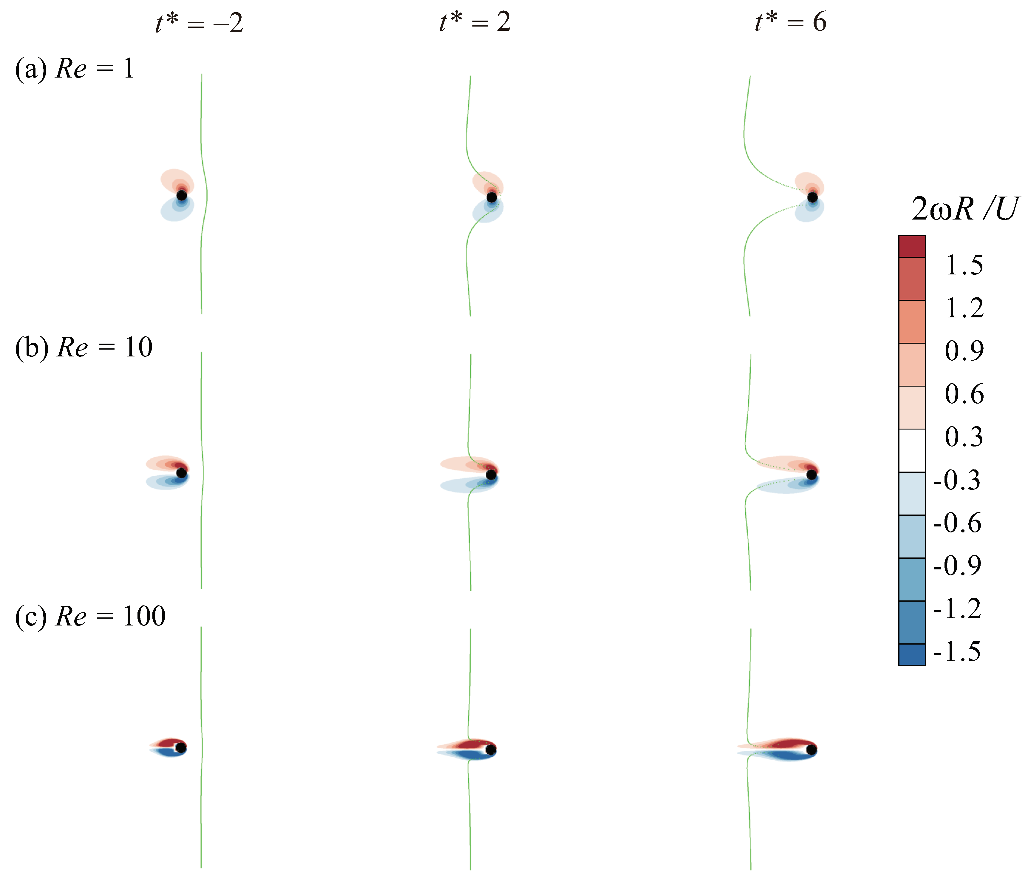
We first examine the effect of Reynolds number on fluid drift for a single cylinder. Although single-cylinder cases are not directly relevant to fluid transport by hairy structures, they are essential in understanding how changes in viscosity influence the behavior of fluid particles. Vorticity fields and particle trajectories are compared for different Reynolds numbers between 1 and 100 in Figure 2. At $Re=1$, vorticity is more widely diffused along the y direction compared with $Re=10$ and $Re=100$. Because of strong viscous diffusion, fluid particles gain more velocity in the region far from the cylinder. As a result, x directional drift occurs for a wider range of the initial material line, and the deformed material line forms an arc-like shape since drift is largest near the cylinder and decreases monotonically in the positive and negative y directions. As the Reynolds number becomes larger, fluid particles near the cylinder are not dragged so much, and, at $Re=100$, the region of drift is almost confined to the diameter of the cylinder.

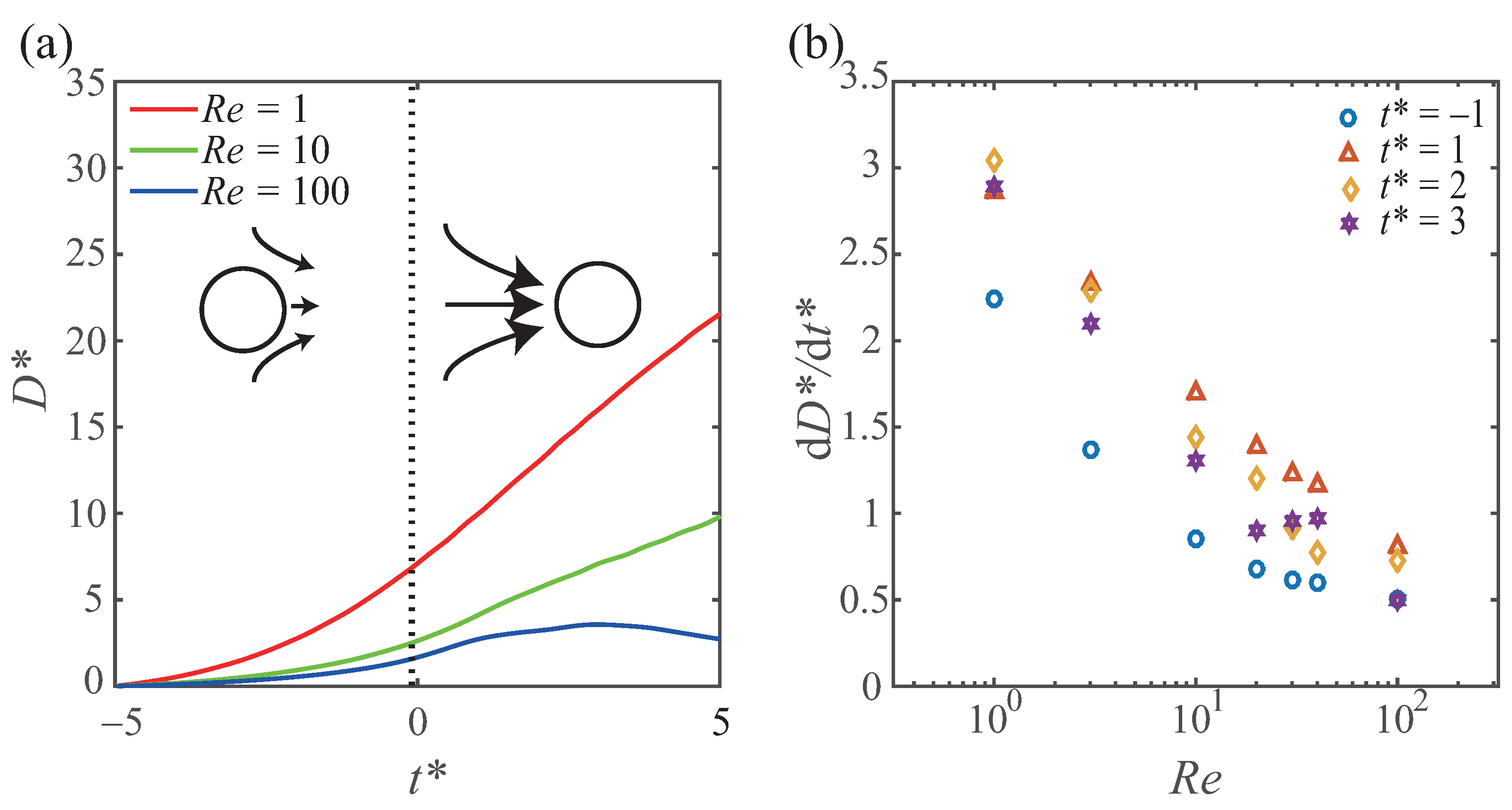
The continuous distortion of the material line leads to temporal variation of the drift volume $D^{*}$ (Figure 3a). For $Re=1$ and $Re=10$ because of the disturbed flow in front of the cylinder, noticeable drift occurs even before the cylinder front touches the initial material line. This is clearly illustrated at $t^{*}=-2$ in Figure 2a. However, drift is more effective when fluid particles are dragged behind the cylinder after $t^{*}=0$, since they are then placed in the region of higher disturbed flow velocity. The slope of $D^{*}$ gradually increases before $t^{*}=0$ and maintains a nearly constant slope after $t^{*}=0$ instead of converging to a specific value at $t^{*}<5$ (Figure 3a). Although not presented here, we have confirmed that, at $Re=1$ and $Re=100$, the slope of $D^{*}$ gradually decreases, but $D^{*}$ does not converge until $t^{*}=35$. This is attributed to fluid particles very close to the cylinder, whose velocities remain comparable to the velocity of the cylinder: $u/U\approx 1$. Although $Re$ is not small enough to expect Stokes-flow behavior, at $Re\le O\left(10\right)$, viscous effects are so strong that the drift volume keeps increasing. On the other hand, at $Re=100$, vorticity is confined to a small y range where the particles are influenced by the rotational motion caused by vortex shedding by the cylinder and tend to head toward the horizontal centerline (Figure 2c). Thus, as time advances, the width of the material line becomes narrower, which leads to a reduction in $D^{*}$ after the cylinder has proceeded a sufficient distance ($t^{*}\approx 3$).

According to Figure 3a, drift volume is inversely related to Reynolds number at a given time, which can also be seen from Figure 2. For example, at $t^{*}=5$, $D^{*}=21.5$ for $Re=1$, which is 2.2 and 7.9 times the values for $Re=10$ and $Re=100$, respectively. Furthermore, Figure 3b shows how viscous effects change the rate of change of drift volume $\mathrm{d}{D}^{*}/\mathrm{d}{t}^{*}$ for $Re\le 100$. The common trend is that, after $t^{*}>0$, $\mathrm{d}{D}^{*}/\mathrm{d}{t}^{*}$ tends to decrease almost linearly with a logarithmic change in $Re$. This linear relation is more obvious at $t^{*}=1$; however, for $t^{*}>1$, deviation is observed, especially at higher Reynolds number.

3.2. Double Cylinders

When two close solid bodies translate side-by-side at low Reynolds number, owing to strong viscous diffusion of vortices (shear layers) generated by the bodies, two counter-rotating vortices in the gap between the bodies will overlap and cancel each other, and the gap will be hydrodynamically blocked by viscous diffusion; i.e., fluids around the bodies rarely penetrate into the gap and behave as if the gap were blocked [12,17]. Such a hydrodynamic barrier is also identified in our double-cylinder model. In Figure 4, the vorticity fields are obtained for $Re=1$–100 at three different time steps. At $Re=1$, counter-rotating vortices inside a gap are annihilated by viscous diffusion and are hardly observed during the time span considered in our study (Figure 4a). Only two vortices outside the cylinders are observed. Because of the hydrodynamic barrier, the material line of fluid particles deforms into an arc shape without any penetration though the gap. The effect of the fluid barrier weakens as the Reynolds number grows. For $Re=10$, fluid particles in front of the cylinders initially drift together, but penetration eventually occurs at around $t^{*}=6$ (Figure 4b). At higher Reynolds number (say, $Re=100$), two counter-rotating vortices are clearly observed inside the gap, and downstream convection of vorticity is prevalent rather than its diffusion. Noticeable penetration of fluid particles results in complicated distortion of the material line (Figure 4c).

In Figure 5, the material lines of entrained fluid particles of moving double cylinders ($Re=1$) for four different gap widths G are illustrated after the double cylinders have passed through the initial material line ($t^{*}=10$). Although the gap-blockage effect is predominant at low Reynolds number ($Re=1$), the deformation of the material line and the magnitude of the drift volume are clearly affected by the gap distance G between the two cylinders (Figure 5). At $G=R$, the material line maintains a convex shape near the cylinders as if it were being drifted by a single connected body. However, with increasing G, penetration of fluid particles begins to occur earlier and the penetration depth becomes greater. Instead of being convex, the material line displays two peaks around the positions of the two cylinders. At a given time, the drift volume increases monotonically with G, but eventually converges, as can be confirmed from the curves of $G=3R$–$5R$ in Figure 5e; as G approaches infinity, which represents the case of two independent cylinders, $D^{*}$ will converge asymptotically to twice the drift volume of a single cylinder.

Further work has been conducted on the penetration of the material line. Here, the penetration time $t_p^{*}$ is defined as the time at which a centerline particle of the material line reaches the same x coordinate as that of the center of the moving cylinders; without any drift, $t_p^{*}=0$. From Figure 5f, we can confirm that $t_p^{*}$ is approximately inversely proportional to $G/R$: $t_p^{*}\sim {(G/R)}^{-1}$. For example, $t_p^{*}=22.8$ for $G=R$ increases sevenfold from the value $t_p^{*}=3.0$ for $G=5R$. The velocity of fluid particles in the gap decays as the double cylinders continue to proceed, and even for small G, penetration eventually occurs, no matter how long this takes.

When the material line (red) of double cylinders is compared with the two superimposed material lines (blue) of a single cylinder for the four cases in Figure 5a–d, two common trends are found. First, regardless of the strong blockage effect at small G or the penetration at large G, the existence of a nearby cylinder induces drift of fluid particles near the centerline ($y^{*}=0$), which results in a gain in the drift volume near the centerline. Second, the material line of the double cylinders is dragged less near $y^{*}=5$ and $-5$ compared with the single-cylinder case, and even undergoes stronger reflux (negative Lagrangian displacement in the x direction) over a wider range, which ends up leading to a loss in drift volume.

For double cylinders, the areas for gain, loss, and overlap in drift volume, relative to the single-cylinder case, are denoted by blue ($D_{\mathrm{gain}}^{*}$), yellow ($D_{\mathrm{loss}}^{*}$), and red ($D_{\mathrm{overlap}}^{*}$), respectively, in Figure 6a. Here, we will quantify the variation of gain and loss volumes by the gap width G. At low Reynolds number ($Re=1$), the material line is symmetric with respect to the centerline, and only the upper half will be evaluated. Instead of the drift volume $D^{*}$ normalized by a single-cylinder area ($\pi r^2$), another dimensionless drift volume $D_{\mathrm{unit}}^{*}$ is used, which is normalized by the total area of two cylinders ($2\pi r^2$). $D_{\mathrm{unit}}^{*}$ is equivalent to the drift volume of the red material line above the centerline in Figure 6a. Then, $D_{\mathrm{unit}}^{*}$ for double cylinders can be expressed as

$$D_{\mathrm{unit}}^{*}=D_{\mathrm{single}}^{*}+D_{\mathrm{gain}}^{*}-D_{\mathrm{loss}}^{*}-D_{\mathrm{overlap}}^{*}.$$

(3)

In Figure 6a and Equation (3), $D_{\mathrm{single}}^{*}$ is the drift volume for the single-cylinder case, and $D_{\mathrm{overlap}}^{*}$ is the area subtracted owing to the overlap of two drift volumes for the single-cylinder case. For any gap width G, $D_{\mathrm{unit}}^{*}$ is smaller than $D_{\mathrm{single}}^{*}$. For example, at $t^{*}=10$, corresponding to Figure 5, $D_{\mathrm{single}}^{*}$ is 31.1 while $D{*}_{\mathrm{unit}}$ is between 24.7 and 29.4 for $G=R$–$5R$. In Figure 6b, $D_{\mathrm{gain}}^{*}$ is greater than $D_{\mathrm{loss}}^{*}$ for all gap widths considered in this study: $D_{\mathrm{gain}}^{*}-D_{\mathrm{loss}}^{*}>0$. Nevertheless, $D_{\mathrm{overlap}}^{*}$ is large enough to offset the net gain ($D_{\mathrm{gain}}^{*}-D_{\mathrm{loss}}^{*}$), and, as a consequence, $D_{\mathrm{unit}}^{*}$ is smaller than $D_{\mathrm{single}}^{*}$.

The monotonic decrease of $D_{\mathrm{overlap}}^{*}$ with increasing G in Figure 6b follows straightforwardly from geometrical considerations; with further separation of the two cylinders, $D_{\mathrm{overlap}}^{*}$ will fall to zero. Meanwhile, the variations of $D_{\mathrm{gain}}^{*}$ and $D_{\mathrm{loss}}^{*}$ with G are quite intriguing in that they rely on the viscous effects of particle drift. As G increases until $G=5R$, the downstream region of the gap expands, contributing to $D_{\mathrm{gain}}^{*}$. However, penetration of the material line proceeds simultaneously and is conspicuous at larger G. For this reason, the rate of increase of $D_{\mathrm{gain}}^{*}$ gradually reduces with G; the rate is found to be 1.4 from $G=R$ to $G=2R$, but only 0.1 from $G=4R$ to $G=5R$ (Figure 6b).

As fluid particles near the centerline drift along the moving cylinders and generate $D_{\mathrm{gain}}^{*}$, reflux should occur at the outer sides of the cylinders in order to satisfy mass conservation (Figure 5a–d). In addition, the vortex at the outer side shown in Figure 4a induces fluid particles behind the cylinders to move toward the centerline, which sequentially causes the material line to recede. Note that the vortex inside the gap is annihilated and cannot counteract the motion of the fluid particles moving toward the centerline. The reflux and the vortex-induced motion of the fluid particles result in recession of the material line and formation of $D_{\mathrm{loss}}^{*}$. In other words, $D_{\mathrm{loss}}^{*}$ is accompanied by $D_{\mathrm{gain}}^{*}$, and they actually show a similar trend in terms of the change in G. Although both $D_{\mathrm{gain}}^{*}$ and $D_{\mathrm{loss}}^{*}$ continue to increase in the range of G tested in this study, they will start to decrease at a certain G and will become zero when the gap-blockage effect disappears and the material line is deformed independently by each cylinder.

3.3. An Array of Cylinders

For a configuration more relevant to biological hairy structures, the collective behavior of an array of cylinders is investigated with respect to material line dynamics and drift volume. In Figure 4, the cases $Re=1$ and $Re=10$ exhibit similar wake patterns: two counter-rotating outer vortices are steadily attached to the cylinders, and two inner vortices are canceled out. If the gap width between the cylinders is small enough (e.g., $G=R$), this wake pattern is reproduced in an array of cylinders, no matter how many cylinders there are: only two counter-rotating outer vortices are steadily sustained, with all inner vortices being smeared out. In this subsection, since similar patterns of flow structure and material line deformation are expected between $Re=1$ and $Re=10$, $Re$ is fixed as 1.

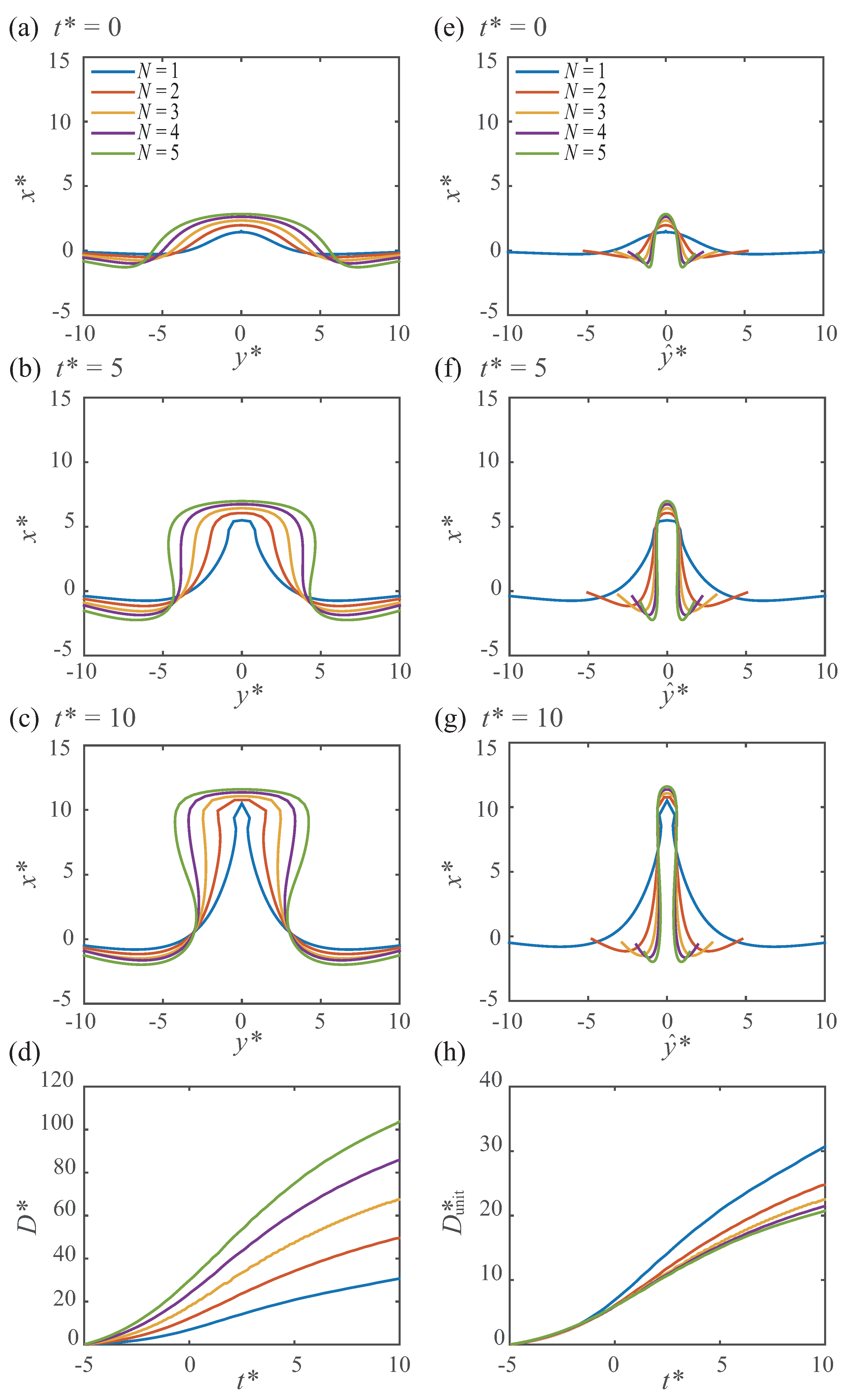
For all cases with different numbers of cylinders considered in this study ($N=1$–5), the shape of the material line shows a noticeable change with increasing N. In Figure 7a–d, the behavior of the material lines for different arrays of cylinders is depicted, and the corresponding drift volumes $D^{*}$ are computed in time series from $t^{*}=-5$ to $t^{*}=10$. The front of the line becomes flatter and drifts slightly faster for larger N. It also becomes wider in the y direction (Figure 7a–c). As a result, $D^{*}$ increases with N as expected (Figure 7d). As cylinders are added one by one, the increment in $D^{*}$ is almost constant in all phases of the translation; i.e., the gap between two adjacent curves in Figure 7d is almost constant at a given time. With increasing N, reflux also increases in accordance with $D^{*}$. Refer to Section 3.2 for the relation between drift volume and reflux. Interestingly, for large N (e.g., $N=5$), the material line near $x=0$ continues to narrow as time advances (Figure 7a,c). Eventually, the width of the material line near $x=0$ becomes almost identical for $t^{*}$ in the range 5–10.

For an array of cylinders, a hydrodynamic barrier is formed inside all the gaps, and the cylinder array can be regarded as a flat plate. The length L from one end of the array to the other is then the dominant factor affecting the overall geometry of the material line. To exclude the effect of length L in the comparison of material lines, the y coordinate is scaled with L rather than with $2R$:

$${\widehat{y}}^{*}=\frac{y}{L}=\frac{y}{N\times 2R+(N-1)\times G}.$$

(4)

As N increases, material lines scaled by L in the y direction tend to approach a single material line (say, the line for $N=5$ in our study) (Figure 7e–g). The collapse of the scaled material lines is clearer in the region close to the cylinder array. Meanwhile, it is noteworthy that the y-directional shrinkage of the scaled material lines with increasing N is observed near $x=0$ far behind the array, which is accompanied by significant reflux as mentioned above.

Asymptotic convergence with increasing N also emerges in the drift volume scaled with N (Figure 7h). In Figure 7h, the drift volume is scaled with the total area of the cylinders rather than with the area of a single cylinder:

$$D_{\mathrm{unit}}^{*}=\frac{D}{N\pi R^2}=\frac{D^{*}}{N}.$$

(5)

whereas $D^{*}$ increases with N, $D_{\mathrm{unit}}^{*}$ decreases with N and converges to the case of large N (say, $N=5$). At $t^{*}=10$, $D_{\mathrm{unit}}^{*}$ decreases by 19.3% from $N=1$ to $N=2$, but by only 3.4% from $N=4$ to $N=5$.

A noticeable trend in Figure 7a–c is that, for large N, the material line near $x=0$ becomes narrower as time goes on, although the material line near the cylinder array remains wide, and this eventually results in the formation of a neck near $x=0$. The width of the material line at $x=0$ decreases about 60% from $t^{*}=0$ to $t^{*}=10$ for $N=5$. The formation of the neck is attributed to counter-rotating outer vortices at both sides of the array.

The velocity fields for each array of cylinders are depicted in Figure 8. Here, u and v components are compared for $N=3$ array at $t^{*}=5$ in Figure 8a, and v components for arrays with different numbers of cylinders are shown at $t^{*}=10$ (Figure 8b–d). Because of the hydrodynamic barrier, the cylinder array produces a homogeneous region of positive u velocity and drags fluids behind the array (Figure 8a). The u velocity is strongest just behind the array and decreases gradually downstream. Large drift in the x direction is accompanied by the formation of strong outer vortices. The outer vortices induce a velocity field with a significant v-velocity component, which results in fluid particles heading toward the centerline $y=0$ (Figure 8a). In Figure 8a, near $x=0$, the maximum $v/U$ is about 0.26, which is comparable to the maximum $u/U$(= 0.26). In Figure 8b–d, on the material line in the wake, the v velocity is not uniform: its magnitude increases gradually from the cylinder array to $x=0$ (in the negative x direction). This nonuniform distribution causes formation of a neck near $x=0$. The v velocity near $x=0$ is stronger for larger N, producing a more noticeable neck.

We have demonstrated that the addition of a cylinder increases the drift volume $D^{*}$ at any time before and after $t^{*}=0$ (Figure 7d). However, this result does not mean that adding a cylinder always contributes to $D^{*}$. In Figure 7, the gap width is fixed as $G=R$ to ensure a strong blockage effect, and the length L from one end to the other (Equation (4)) is varied. On the other hand, let us consider fixed L for the two outermost cylinders and place additional cylinders between these two, thereby increasing N. In this scenario, with increasing N, the overall blockage effect will continue to become stronger, either by direct obstruction of flow due to the added cylinders or by enhancement of the fluid barrier due to the narrower gap width G. For finite L, the space between two adjacent cylinders will eventually become blocked with further increase in N. Thus, as N increases, the effect of the blocking behavior on drift volume will become negligible.

To find the relation between drift volume and number of cylinders for fixed length L, we first position two cylinders with $G=10R$ and then examine the changes in the material line and drift volume when additional cylinders are placed between them such that the cylinders are equally spaced and G between two adjacent cylinders is varied: $N=2$ ($G=10R$), $N=3$ ($G=4R$), $N=4$ ($G=2R$), and $N=5$ ($G=R$) (Figure 9a,b). In contrast to Figure 7, which exhibits similarity of material lines when they are scaled with ${\widehat{y}}^{*}(=y^{*}/L)$, variation of G allows different behaviors of the penetrability through the gap, which breaks the geometric similarity near the cylinder array. In Figure 9a,b, fluid penetration through the gap occurs for $N=2$ and $N=3$, while complete blockage of the gap is observed for $N=4$ and $N=5$. The time history of $D^{*}$ in Figure 9c also shows an irregular pattern. Because of the formation of irregular material lines for the four cases, in contrast to Figure 7d, which exhibits a linear increase in $D^{*}$ with increasing N, the increase in $D^{*}$ is not regular. That is, the spacing between the curves for $N=2$–5 is not uniform (Figure 9c).

Interestingly, the front of the material line for $N=4$ proceeds slightly faster than that for $N=5$ (Figure 9a,b). In the meantime, the neck near $x=0$ recedes faster toward the centerline. The trend at the front is opposite to the trend observed in Figure 7; compare the material lines for $N=4$ and $N=5$ between Figure 7 and Figure 9. Because of the more rapid advancement of the front, the drift volume for $N=4$ can be even larger than that for $N=5$ from $t^{*}=-5$ to $t^{*}=2.6$ (Figure 9c).

In addition to $D^{*}$, $D_{\mathrm{unit}}^{*}$ also exhibits irregular behavior without uniform convergence with increasing N, in contrast to Figure 7h (Figure 9d). Noticeably, while $D_{\mathrm{unit}}^{*}$ for $N=3$ is always smaller than that for $N=2$ in Figure 7h, $D_{\mathrm{unit}}^{*}$ for $N=3$ is always larger than that for $N=2$. This trend is mainly because the material line for $N=3$ exhibits much smaller penetration at the gaps, leading to larger $D_{\mathrm{unit}}^{*}$ as well as $D^{*}$. Furthermore, $D_{\mathrm{unit}}^{*}$ for $N=4$ exceeds the other cases for a finite time span ($t^{*}<0$), owing to the more rapid advance of the front material line as mentioned above.

In this study, we have adopted drift volume to evaluate the efficiency of fluid transport, and admittedly we could have considered another parameter suitable for a given problem. Nevertheless, the results in Figure 9c,d indicate that, for a given condition (say, fixed L in our study), there may be an optimal number (and configuration) of solid bodies to effectively transport fluid volume around them, and this optimal number will depend on how we define the effectiveness: for example, $D^{*}$ or $D_{\mathrm{unit}}^{*}$ in our study.

4. Conclusions

We have numerically investigated fluid transport induced by translating motion of two-dimensional cylinders, which is inspired by transport phenomena found in biological hairy structures for olfactory sensing and food capture. Strong viscous diffusion at low Reynolds number allows more fluid to drift along a cylinder, and a material line composed of fluid particles that is initially straight and perpendicular to the direction of motion of the cylinder deforms into an arc shape. When multiple cylinders translate, viscous diffusion may prevent penetration of fluid through the gaps between cylinders. The material line then deforms as if the cylinder array were a continuous flat plate. As the number of cylinders increases, if the material line is properly scaled with the total length of the cylinder array, it converges to a specific shape that has nonuniform width downstream of the array. Accordingly, the drift volume per total cylinder area decreases with increasing number of cylinders, and asymptotically approaches a specific value. The collective interaction of a moving cylinder array due to strong viscous effects suggests that the configuration of the array could be optimized to enhance the efficiency of fluid transport.

In this study, to allow quantification of fluid transport under various conditions, as well as analysis of its characteristics, we have simplified the model as comprising two-dimensional cylinders and have focused on the temporal deformation of a fluid material line and the temporal change in drift volume. Although this study provides insight into the collective performance of fluid transport in a low Reynolds-number flow, in order to elucidate the collective hydrodynamic behavior of the hairy structures that occur in nature and its biological implications, we should consider more elaborate physical models and transport phenomena coupled with the convection and diffusion of chemicals and the dynamics of inertial particles. These are left as topics for our future work.

References

1. Atema, J. Aquatic and terrestrial chemoreceptor organs: Morphological and physiological designs for interfacing with chemical stimuli. In Comparative Physiology: Life in Water and on Land; Springer: Berlin/Heidelberg, Germany, 1987; pp. 303–316. [Google Scholar]
2. Koehl, M. Small-scale fluid dynamics of olfactory antennae. Mar. Freshw. Behav. Phy. 1996, 27, 127–141. [Google Scholar] [CrossRef]
3. Koehl, M.; Koseff, J.R.; Crimaldi, J.P.; McCay, M.G.; Cooper, T.; Wiley, M.B.; Moore, P.A. Lobster Sniffing: Antennule Design and Hydrodynamic Filtering of Information in an Odor Plume. Science 2001, 294, 1948–1951. [Google Scholar] [CrossRef] [PubMed]
4. Crimaldi, J.; Koehl, M.; Koseff, J. Effects of the Resolution and Kinematics of Olfactory Appendages on the Interception of Chemical Signals in a Turbulent Odor Plume. Environ. Fluid. Mech. 2002, 2, 35–64. [Google Scholar] [CrossRef]
5. Shimeta, J.; Jumars, P.A. Physical mechanisms and rates of particle capture by suspension-feeders. Oceanogr. Mar. Biol. Annu. Rev 1991, 29, 191–257. [Google Scholar]
6. Winter, J.E. A review on the knowledge of suspension-feeding in lamellibranchiate bivalves, with special reference to artificial aquaculture systems. Aquaculture 1978, 13, 1–33. [Google Scholar] [CrossRef]
7. Morris, M.; Gust, G.; Torres, J. Propulsion efficiency and cost of transport for copepods: A hydromechanical model of crustacean swimming. Mar. Biol. 1985, 86, 283–295. [Google Scholar] [CrossRef]
8. Button, B.; Cai, L.H.; Ehre, C.; Kesimer, M.; Hill, D.B.; Sheehan, J.K.; Boucher, R.C.; Rubinstein, M. A periciliary brush promotes the lung health by separating the mucus layer from airway epithelia. Science 2012, 337, 937–941. [Google Scholar] [CrossRef] [Green Version]
9. Faubel, R.; Westendorf, C.; Bodenschatz, E.; Eichele, G. Cilia-based flow network in the brain ventricles. Science 2016, 353, 176–178. [Google Scholar] [CrossRef]
10. Nawroth, J.C.; Guo, H.; Koch, E.; Heath-Heckman, E.A.; Hermanson, J.C.; Ruby, E.G.; Dabiri, J.O.; Kanso, E.; McFall-Ngai, M. Motile cilia create fluid-mechanical microhabitats for the active recruitment of the host microbiome. Proc. Natl. Acad. Sci. USA 2017, 114, 9510–9516. [Google Scholar] [CrossRef] [Green Version]
11. Feitl, K.; Millett, A.; Colin, S.; Dabiri, J.O.; Costello, J.H. Functional Morphology and Fluid Interactions During Early Development of the Scyphomedusa Aurelia aurita. Biol. Bull. 2009, 217, 283–291. [Google Scholar] [CrossRef] [Green Version]
12. Lee, S.H.; Kim, D. Aerodynamics of a translating comb-like plate inspired by a fairyfly wing. Phys. Fluids 2017, 29, 081902. [Google Scholar] [CrossRef]
13. Lee, S.H.; Lahooti, M.; Kim, D. Aerodynamic characteristics of unsteady gap flow in a bristled wing. Phys. Fluids 2018, 30, 071901. [Google Scholar] [CrossRef]
14. Nawroth, J.; Feitl, K.; Colin, S.; Costello, J.H.; Dabiri, J. Phenotypic plasticity in juvenile jellyfish medusae facilitates effective animal–fluid interaction. Biol. Lett. 2010, 6, 389–393. [Google Scholar] [CrossRef] [PubMed]
15. Santhanakrishnan, A.; Robinson, A.; Jones, S.; Low, A.; Gadi, S.; Hedrick, T.; Miller, L. Clap and fling mechanism with interacting porous wings in tiny insect flight. J. Exp. Biol. 2014, 217, 3898–3909. [Google Scholar] [CrossRef] [Green Version]
16. Jones, S.K.; Yun, Y.J.; Hedrick, T.L.; Griffith, B.E.; Miller, L.A. Bristles reduce the force required to ‘fling’wings apart in the smallest insects. J. Exp. Biol. 2016, 219, 3759–3772. [Google Scholar] [PubMed] [Green Version]
17. Cheer, A.; Koehl, M. Paddles and rakes: Fluid flow through bristled appendages of small organisms. J. Theor. Biol. 1987, 129, 17–39. [Google Scholar] [CrossRef]
18. Spielman, L.A. Particle capture from low-speed laminar flows. Ann. Rev. Fluid Mech. 1977, 9, 297–319. [Google Scholar]
19. Darwin, C. Note on hydrodynamics. In Mathematical Proceedings of the Cambridge Philosophical Society; Cambridge University Press: Cambridge, UK, 1953; Volume 49, pp. 342–354. [Google Scholar]
20. Sumner, D. Two circular cylinders in cross-flow: A review. J. Fluids Struct. 2010, 26, 849–899. [Google Scholar] [CrossRef]
21. Lin, Z.; Zhang, Y. Stirring by multiple cylinders in potential flow. J. Fluid Mech. 2016, 794, 552–564. [Google Scholar] [CrossRef] [Green Version]
22. Matsumoto, G. Swimming movements of ctenophores, and the mechanics of propulsion by ctene rows. Hydrobiologia 1991, 216, 319–325. [Google Scholar] [CrossRef]
23. Barlow, D.; Sleigh, M.A.; White, R.J. Water flows around the comb plates of the ctenophore Pleurobrachia plotted by computer: A model system for studying propulsion by antiplectic metachronism. J. Exp. Biol. 1993, 177, 113–128. [Google Scholar]
24. Dauptain, A.; Favier, J.; Bottaro, A. Hydrodynamics of ciliary propulsion. J. Fluids Struct. 2008, 24, 1156–1165. [Google Scholar] [CrossRef] [Green Version]
25. Gilmanov, A.; Sotiropoulos, F. A hybrid Cartesian/immersed boundary method for simulating flows with 3D, geometrically complex, moving bodies. J. Comput. Phys. 2005, 207, 457–492. [Google Scholar] [CrossRef]
26. Saad, Y.; Schultz, M.H. GMRES: A Generalized Minimal Residual Algorithm for Solving Nonsymmetric Linear Systems. SIAM J. Sci. Stat. Comput. 1986, 7, 856–869. [Google Scholar] [CrossRef] [Green Version]
27. Brown, P.N.; Saad, Y. Hybrid Krylov Methods for Nonlinear Systems of Equations. SIAM J. Sci. Stat. Comput. 1990, 11, 450–481. [Google Scholar] [CrossRef]
28. Van Kan, J. A Second-Order Accurate Pressure-Correction Scheme for Viscous Incompressible Flow. SIAM J. Sci. Stat. Comput. 1986, 7, 870–891. [Google Scholar] [CrossRef]
29. Ge, L.; Sotiropoulos, F. A numerical method for solving the 3D unsteady incompressible Navier–Stokes equations in curvilinear domains with complex immersed boundaries. J. Comput. Phys. 2007, 225, 1782–1809. [Google Scholar] [CrossRef] [PubMed] [Green Version]
30. Eames, I.; Belcher, S.; Hunt, J. Drift, partial drift and Darwin’s proposition. J. Fluid Mech. 1994, 275, 201–223. [Google Scholar] [CrossRef] [Green Version]
31. Eames, I.; Gobby, D.; Dalziel, S. Fluid displacement by Stokes flow past a spherical droplet. J. Fluid Mech. 2003, 485, 67–85. [Google Scholar] [CrossRef] [Green Version]
32. Dabiri, J.O. Note on the induced Lagrangian drift and added-mass of a vortex. J. Fluid Mech. 2006, 547, 105–113. [Google Scholar] [CrossRef] [Green Version]
33. Katija, K.; Dabiri, J.O. A viscosity-enhanced mechanism for biogenic ocean mixing. Nature 2009, 460, 624–626. [Google Scholar] [CrossRef] [PubMed] [Green Version]
34. Pushkin, D.O.; Shum, H.; Yeomans, J.M. Fluid transport by individual microswimmers. J. Fluid Mech. 2013, 726, 5–25. [Google Scholar] [CrossRef] [Green Version]
35. Chisholm, N.G.; Khair, A.S. Drift volume in viscous flows. Phys. Rev. Fluids 2017, 2, 064101. [Google Scholar]
36. Chisholm, N.G.; Khair, A.S. Partial drift volume due to a self-propelled swimmer. Phys. Rev. Fluids 2018, 3, 014501. [Google Scholar] [CrossRef]
Figure 1. Schematics of the cylinder model: (a) single cylinder and (b) double cylinders. The dashed vertical line is the initial material line composed of fluid particles (circles), and the solid line is the deformed material line at a specific time.
Fluids 05 00005 g001
Figure 2. Vorticity contours and distortion of a material line for a single cylinder at three instants: (a) R e = 1 ; (b) R e = 10 ; and (c) R e = 100 . See Supplementary Video S1.
Fluids 05 00005 g002
Figure 3. (a) time history of dimensionless drift volume D * (Equation (2)) for a single cylinder; (b) rate of increase of drift volume d D * / d t * as a function of Reynolds number at several instants.
Fluids 05 00005 g003
Figure 4. Vorticity contours and distortion of a material line for double cylinders at three instants: (a) R e = 1 ; (b) R e = 10 ; and (c) R e = 100 . The gap width G is equal to the cylinder radius R (Figure 1). See Supplementary Video S2.
Fluids 05 00005 g004
Figure 5. (ad) material line of fluid particles (red line) at t * = 10 for double cylinders ( R e = 1 ): (a) G = R ; (b) G = 2 R ; (c) G = 4 R ; and (d) G = 5 R . The blue line is the material line of the single-cylinder case at the same time ( t * = 10 ), which is indicated with respect to the current position of each cylinder: there are two separate blue lines for each cylinder. Note that the x * and y * axes are reversed: x * = x / ( 2 R ) and y * = y / ( 2 R ) ; (e) time history of drift volume D * for G = R 5 R ; (f) penetration time of a fluid particle at the center ( y * = 0 ) of a material line.
Fluids 05 00005 g005
Figure 6. (a) drift volume gain D gain * , loss D loss * , and overlap D overlap * for double cylinders; the red line is for double cylinders and the two identical blue lines are for a single cylinder; (b) variation of D gain * and D loss * with gap width G at t * = 10 ( R e = 1 ).
Fluids 05 00005 g006
Figure 7. (ac) material line deformation for different numbers of cylinders ( N = 1 –5, G = R ) at (a) t * = 0 ; (b) t * = 5 ; and (c) t * = 10 . Note that the x * and y * axes are reversed: x * = x / ( 2 R ) and y * = y / ( 2 R ) ; (d) time history of drift volume D * for N = 1 –5; (eg) material line deformation scaled by the new y ^ * coordinate (Equation (4)); (h) time history of drift volume D unit * (Equation (5)); (eh) correspond to (ad), respectively.
Fluids 05 00005 g007
Figure 8. (a) contours of (i) u velocity ( u / U ) and (ii) v velocity ( v / U ) for a cylinder array at t * = 5 for N = 3 . The vertical dashed line is the initial material line at x = 0 ; (be) contours of v velocity ( v / U ) for a cylinder array at t * = 10 for (b) N = 2 ; (c) N = 3 ; (d) N = 4 ; and (e) N = 5 . The black lines with arrows indicate the relative size and direction of rotation of the outer vortices.
Fluids 05 00005 g008
Figure 9. (a,b) material line deformation for different numbers of cylinders ( N = 2 –5) at (a) t * = 0 and (b) t * = 5 . The gap between the two outermost cylinders is fixed as G = 10 R . Note that the x * and y * axes are reversed; (c,d) time histories of (c) drift volume D * and (d) drift volume D unit * for N = 2 –5.
Fluids 05 00005 g009