1. Introduction
Microscopic multiphase flows facilitate a wide field of possible applications since they provide short diffusion layers within the flow structures. This enables high mass and heat transfer rates [
1,
2] for several applications ranging from extraction [
3] and multiphase catalyst reactions [
4] to improved unit operations such as mixing tasks [
5]. The distinct features allow performing reactions at new process windows with fewer hazards or higher selectivity [
6]. The specific flow conditions can furthermore serve for cell isolation [
7], genetic analysis [
8] and reaction screening in a droplet chain [
9]. In contrast to large scale multiphase flows, microscopic flows are much easier to predict as there are no complex interactions such as swarm turbulence [
10,
11] commonly found in bubble columns. In fact, the reproducibility of Taylor flows is a key for the application of microscopic multiphase flows [
12].
In the Taylor flow regime, the disperse phase is separated from the wall by a thin wall film and does not fill the entire cross-section of the microchannel. The remaining space between the droplet and the microchannel’s corners is occupied by the continuous phase, which is referred to as gutters [
13]. The droplets are typically longer than the channel diameter, which leads to separated elongated disperse phase instances. The continuous phase segments between the droplets are called slugs. Taylor flows are mainly established in circular capillaries or rectangular microchannels whereas especially the hydrodynamics of moving Taylor droplets in circular capillaries and the role of the thin wall film have been intensively studied [
14].
Chemical reactions on the microscale are often performed in monolith reactors functioning as as a catalyst support. In these reactors, a high number of parallelized channels with hexagonal or square channel cross-section offer a high specific reaction area for wall placed catalysts at small wall thickness. This results in a better heat transfer through the walls and better mechanical stability than circular capillaries [
15]. For process control and stabilization, as well as precise reactor design, knowledge of the underlying fluidic terms is crucial. The high grade of parallelity complicates the prediction of the hydrodynamics and the resulting pressure drop [
16,
17].
Besides disperse phase size distribution and formation frequency [
18], the actual droplet velocity is essential for the droplet residence time in the reactor. It determines the contact time of the educts and influences the pressure drop of the reactor [
19]. In parallel reactors, the exact knowledge of the pressure drop is especially necessary since a steady educt supply for each individual single reactor is needed to ensure stable and efficient working conditions [
20].
Several publications deal with the droplet velocity in rectangular capillaries and observe a droplet velocity mostly faster than the superficial velocity (see
Section 3). For flows in circular capillaries, where only a thin wall film is present, this velocity difference is well understood [
21], while for rectangular microchannels a variety of explanations exist, which mostly correlate the relations from measurements [
22]. This complicates the transfer of results to other flow applications or altered process parameters since local and instantaneous hydrodynamic parameters are mostly not taken into account by the models and correlations.
This work aims to establish a model to determine the droplet velocity from the actual flow conditions [
23]: e.g., droplet length, material properties, and the
number. In a first step, we develop a concept for the relative droplet velocity, which bases this velocity on extrinsic parameters, allowing a linear scaling. From this concept, we identify the bypass flow through the gutters as well as the film-thickness as the prominent parameters for the excess velocity.
In the next step, we develop a model that uses the local surface curvature of the gutters to retrieve the local pressure at the entrance and outlet of the gutter as a driving force. The bypassing gutter flow is calculated based on the counterplay of this driving force, the gutter length and a viscosity correlated resistance factor
. The local droplet curvature at the gutter entrances is derived with an analytical interface shape approximation [
24] and a correlation for the droplet cap curvature based on the
number from our previous work [
25]. The model was successfully validated using high-speed camera measurements.
2. Hydrodynamic Fundamentals of Taylor Flows
The Taylor flow regime in rectangular microchannels is mainly influenced by surface tension forces rather than inertia forces. In the Taylor flow regime, a droplet fills nearly the whole cross-section of a hydrodynamic channel, while the continuous phase occupies the gutters and a thin wall film. The droplets are divided by the slugs, consisting only of liquid from the continuous phase.
The interaction between interfacial and viscous forces is described by the Capillary number
.
Herein,
represents the dynamic viscosity of the continuous phase,
the interfacial tension between both phases and
the total superficial flow velocity:
The superficial velocity is based on the volume flow of the disperse and continuous phase as well as the microchannel’s cross-sectional area that calculates from the channel width W and channel height H or, respectively, the channel aspect ratio .
For energetic considerations, knowledge of the ratio between inertia and viscous forces is of importance. The Reynolds number
is used to describe the ratio between inertia and viscous forces of the continuous phase with
being the continuous phase density and
the continuous phase viscosity. Additionally, the viscosity ratio
between both phases has a significant influence on the pressure drop and the velocity of a droplet [
19,
26,
27] since it indicates the momentum coupling into the disperse phase. Please note that the definition of
differs in the mentioned publications.
Considering the overall classification of the applied flow system, the material properties of both fluid phases are of importance. The Ohnesorge number
describes the most prominent material properties for droplets being formed or dispersed [
28]. It characterizes the fluidic system independent of current flow or forces and is mostly used when working with surfactants to manipulate the flow properties. Here, we use the
number to characterize the continuous phase.
In many applications, Taylor droplets in rectangular microchannels move with a velocity different from the superficial velocity, because the droplet does not fill the entire channel cross-section and continuous phase can bypass the droplet through the gutters. An early description was given by Wong et al. [
29], who described these phenomena analytically and declared two possible regimes.
In the first regime, the fluid in the gutters moves slower than the droplet, dissipating kinetic energy. For the gutters, Abiev [
21] reported an inverted pressure gradient, indicated by the local surface curvature. For circular microchannels, this results in an inverse flow of the wall film and the droplet moves faster than the superficial velocity.
In the second flow regime, which holds true for long and highly viscous droplets [
27,
29,
30], more energy is dissipated through the larger wall film area and through viscous dissipation in the droplets. Consequently, the flow in the gutters moves from the droplet back to the front. Thus, the droplet moves slower than the superficial velocity.
For both regimes, the thin wall film resists the motion of the droplet, resulting in a difference in pressure with higher value at the back and a lower value at the front of the droplet. The transition between both regimes is described by a critical flow rate and depends on the droplet length and the channel aspect ratio [
29].
Jakiela et al. [
31] focused experimentally on the influence of the momentum coupling between both phases represented by
and also revealed a dependence of the droplet velocity on the droplet length. For short, low viscous droplets (
), the droplets move faster than the superficial velocity and the droplet behavior is assigned to the first flow regime. Highly viscous droplets (
) move either faster or slower than the superficial velocity, depending strongly on the droplet length.
3. Concept of Excess Velocity
Based on the instantaneous droplet velocity
, which is evident and directly measurable via optical or electrical measurement techniques [
32], different explanatory approaches for the deviation of superficial velocity
and droplet velocity
have been reported.
Liu et al. [
33] defined this relative difference as slipping velocity
, Howard and Walsh [
34] as relative drift velocity
, Angeli and Gavriilidis [
35] as relative bubble velocity
and Abadie et al. [
36] as dimensionless droplet velocity. Jakiela et al. [
31] focused directly on the ratio of
and named this quotient droplet mobility according to Bretherton [
37]. For this work, we summarize these approaches as a slipping velocity:
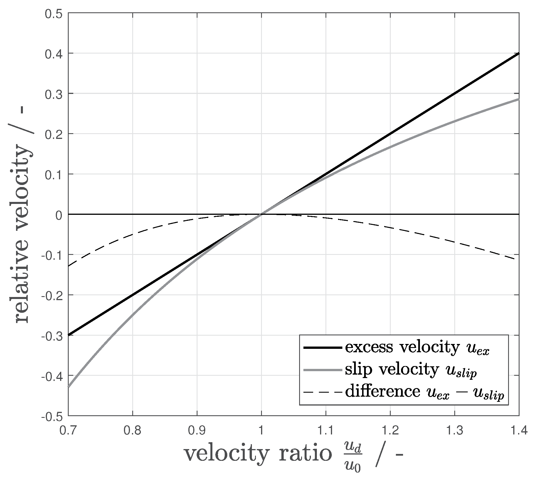
In those concepts, the desired quantity is scaled with an intrinsic value such as the instantaneous droplet velocity, which leads to normalization effects as values
and
are not normalized symmetrically (
Figure 1). This behavior has to be taken into account when experimental or simulative data is interpreted.
In our approach, we scale the velocity difference with the superficial velocity as an extrinsic property and, staying in the terms of extrinsic denomination, define it as an excess velocity
In this manner, results values around 0 for droplet velocities equal to the superficial velocity (plug flow), while positive and negative values indicate droplets that are, compared to the superficial velocity, faster or slower, respectively.
The advantage of this extrinsic concept stands out in a comparison of both approaches (
Figure 1). The first shown intrinsic concept (slip velocity) leads to an asymmetrical scaling behavior, especially for droplets with
, since
decreases more strongly than
would increase. For applications such as balancing or process modeling, a linear behavior of ratio values is preferable to simplify the balances. Otherwise, the nonlinear behavior would lead to an additional bias towards any direction
, which requires a nonlinearly compensation in the description of the phenomena and complicates the model development.
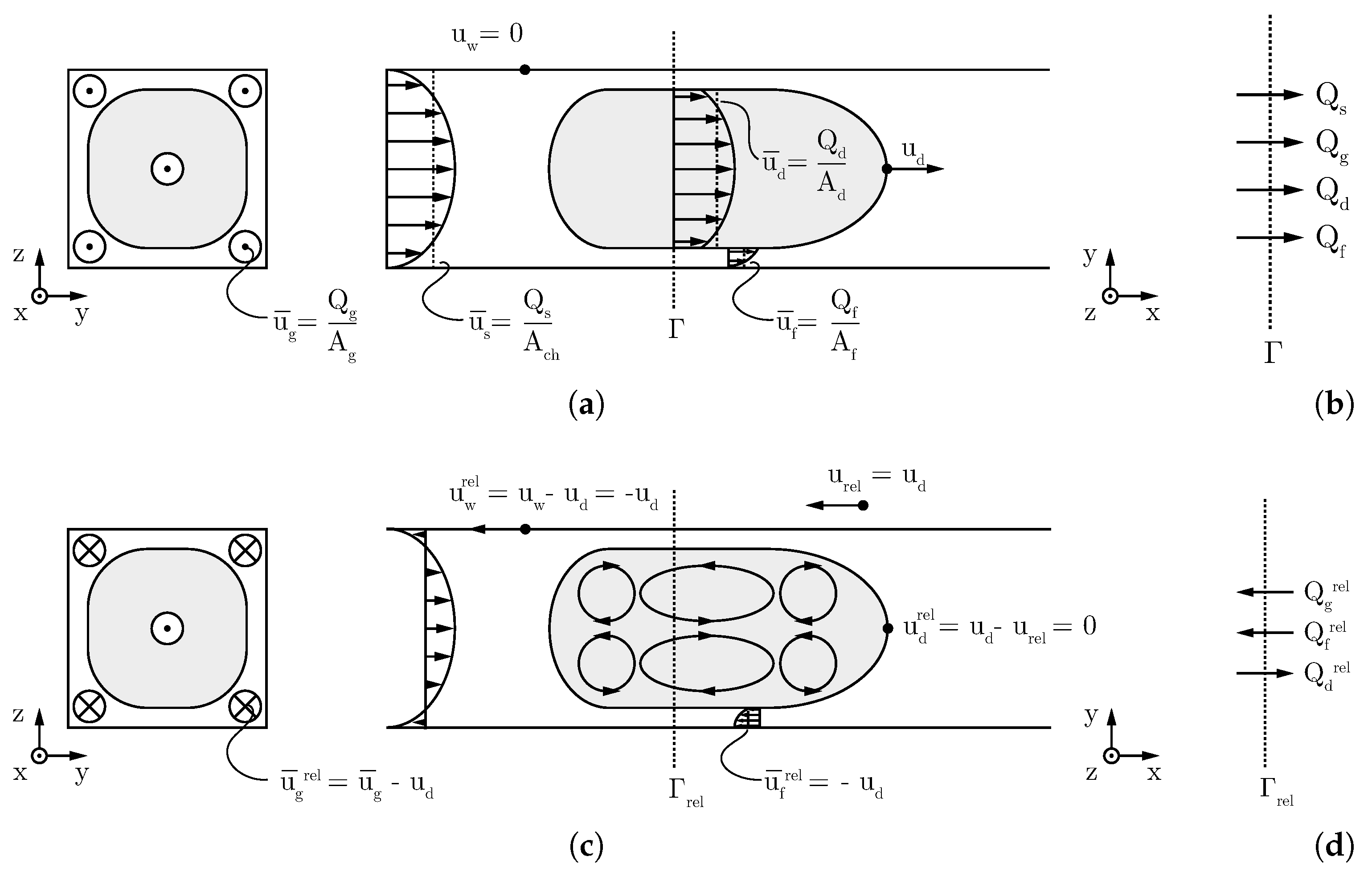
A description for the excess velocity can be derived from the volume flows around moving droplets (Equation (
8)). The continuity equation describes the connection between the gutter flow and the outer driving flows and delivers the relation between the total flow
and the volume flow fractions of the disperse
as well as the continuous phase
. Considering the unit cell of a single slug and an adjoining droplet, the continuous phase divides into the volume flow of the slug (
), the flow through the gutters (
), and through the wall film (
):
If we depict the flows at a moving Taylor droplet (
Figure 2a) and introduce a stationary control surface
(
Figure 2b), velocities can be retrieved from the balances, while two different flow states are possible: In the case of a droplet passing
, the slug volume flow through the control surface is
(since there is no slug present). For a slug passing
, only the slug volume
is present. As one can see, the use of a stationary point of view leads to nonstationary terms in the balances.
If the coordinate system is changed from a fixed frame to a moving frame by moving the control surface with an arbitrary velocity
, the balances become stationary and relative velocities become visible (
Figure 2c). For this moving coordinate system, an additional volume flow
adds to the balances that result from the transformation of the coordinate system (
Figure 2d):
This changes Equation (
8) to:
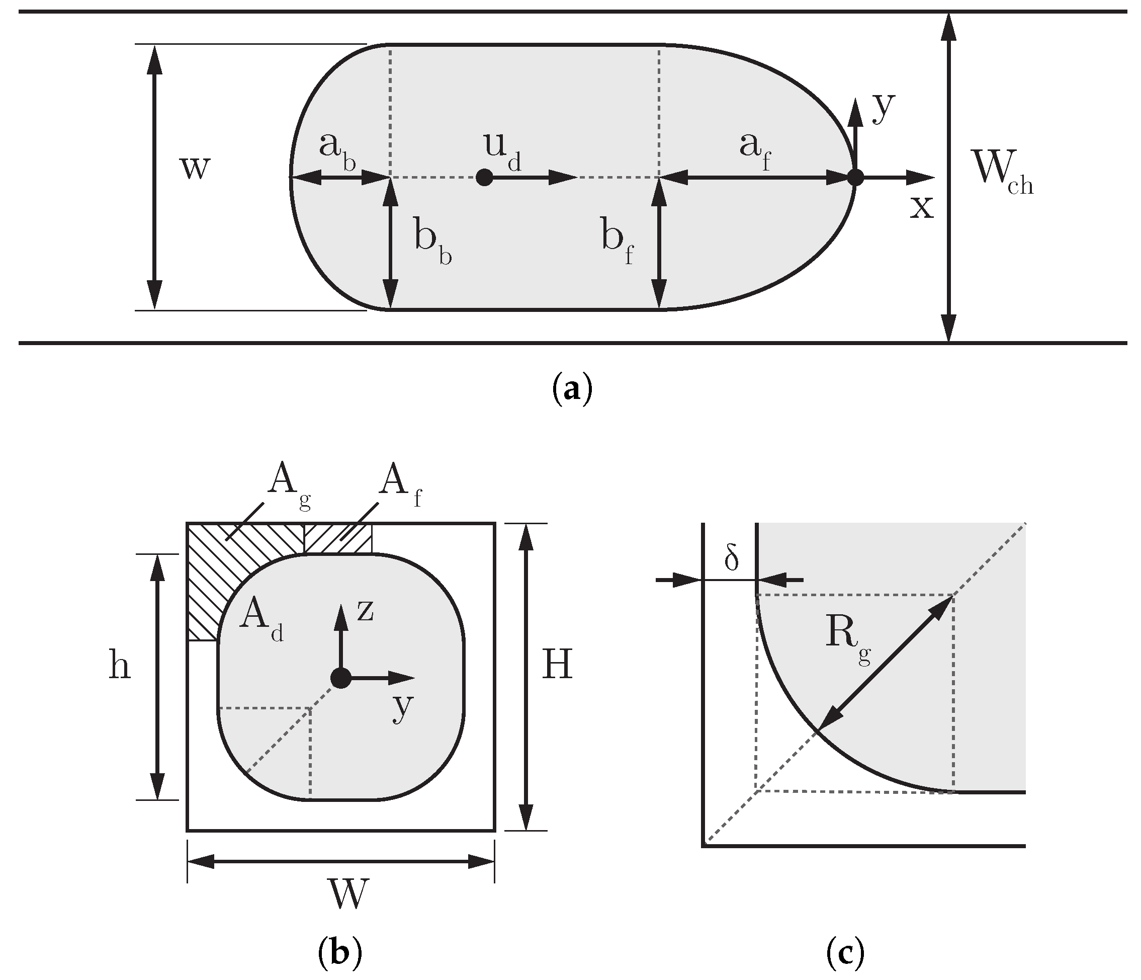
With knowledge of the specific areas for each distinct volume flow rate, the averaged velocities can be calculated. Following
Figure 3a,c, we conclude for the gutter area
of all four gutters
with
denoting the wall film-thickness and
representing the mean dynamic gutter radius, which is described below in
Section 4. For the cross-sectional film area
, we state with the aspect ratio
The droplet cross-sectional area
is delivered combining
and
:
With the cross-sectional areas of the droplet, the gutter and the wall film, the volume flow rates can be rearranged to area-averaged velocities and Equation (
10) becomes
Herein, , and are area-averaged velocities of the droplet, gutter and film, respectively.
For the droplet (
) and the film volume flow (
), the transition velocity
equals the stagnation point velocity
, since we assume incompressibility, mass conservation, a stagnant film and a stationary droplet shape [
38].
Additionally, we assume the averaged velocity in the thin wall films to be insignificant for
Therefore, Equation (
14) simplifies to
Herein,
represents the relative gutter velocity, which dissipates flow energy in the gutter. Simplification and combination with Equation (
7) leads to
We neglect the terms that are small of higher-order (see
Appendix A) and retrieve an expression for the excess velocity:
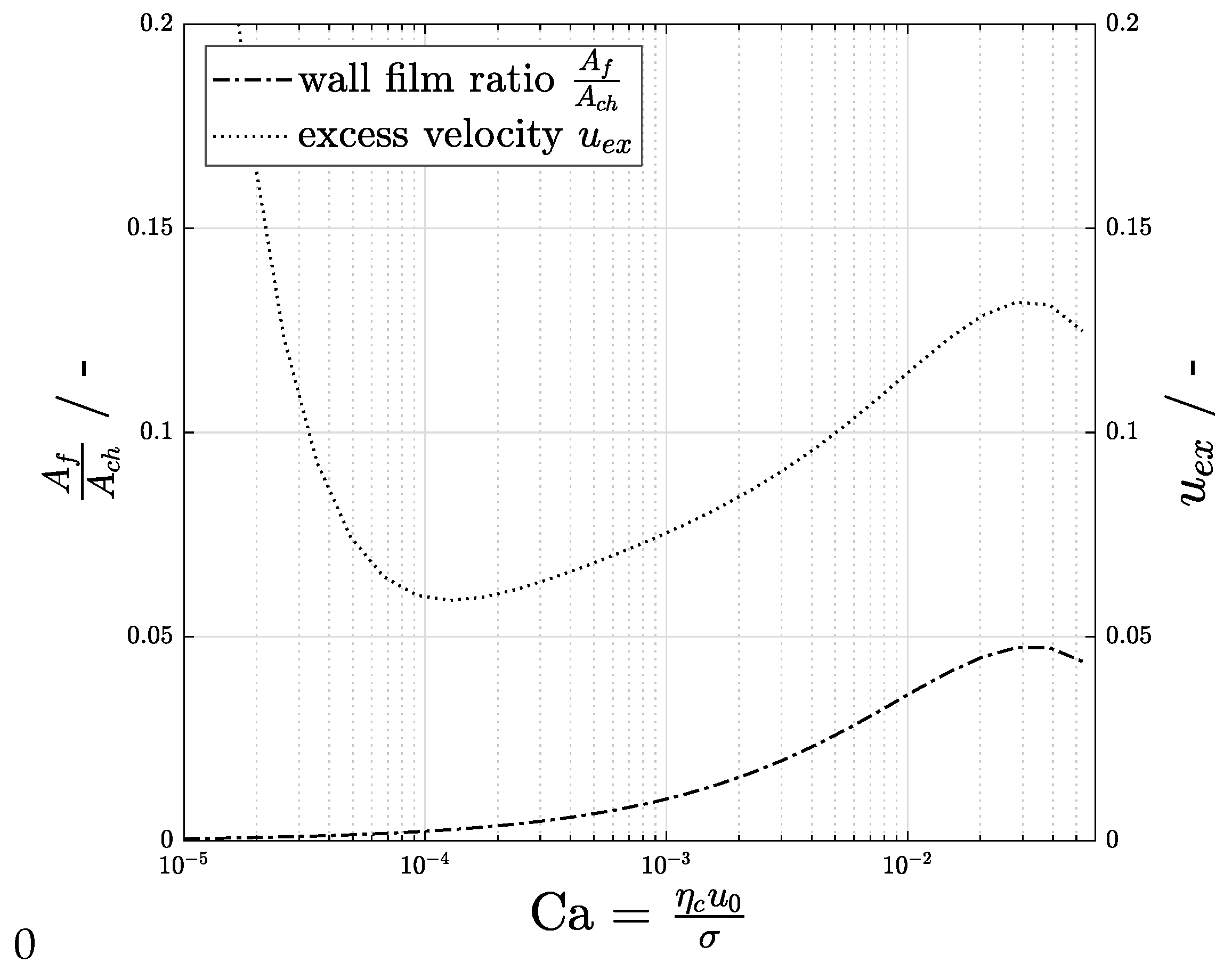
The relative gutter volume flow () and the cross-sectional area of the wall film are the most prominent influencing quantities for the excess velocity. Thus, our proposed model aims to especially determine these quantities.
4. Model Specification
The considerations of the previous section identify the volume flows, which determine the excess velocity. In a second step, we clarify the relevant influential parameters on these volume flows and their interconnection.
For the proposed modeling approach, we adapt a greybox model following Hangos and Cameron [
39]. Our model is developed from engineering principles, hydrodynamic considerations (see
Section 3) and well-defined equations, whereas the initialization of a part of the influential parameters is based on measured data. The underlying relations can be described as an intermediate concept between a black box (completely based on measurement data) and a white box model (based only on analytically well-known equations and engineering principles).
As depicted in
Section 3, we assume a droplet flowing through a rectangular microchannel with its properties according to
Figure 3. The thin wall film cross-section
is determined by Equation (
12) and depends on the channel height
H, the channel aspect ratio
and the film-thickness
. To determine
, we apply the model of Han and Shikazono [
40], which holds for
. For the proposed excess velocity model, full wettability of the walls with a stable wall film is assumed. Besides this behavior being proven in the later measurements (see
Section 6), we compared this assumption with the literature. Kreutzer et al. [
41] analytically retrieved the counterplay of film rupture in the region near the gutters and film formation at the bubble or droplet front. Furthermore, they found coherences for the length where the film starts to rupture. For short or fast droplets, new films are formed more quickly than they rupture. In this work, mainly short droplets are covered.
Khodaparast et al. [
42] focused on the dewetting of the wall film and found a distance from the droplet front, at which dewetting occurs, to correlate with Ca in the range
and the surface wettability. As a criterion, they found a minimum film-thickness of 100 nm, beyond which rupture is suppressed. For the presented range of the model (
,
), based on the film thickness model of Han and Shikazono [
40], the critical film-thickness never drops below this value.
For the flow of the bulk phase as well as the flow in the gutters, we omit the influence of viscous heating based on the criterion of Morini [
43]. We elaborate on this in
Appendix B.
The relative volume flow through the gutter
is derived from the pressure difference along the gutters, as suggested by Abiev [
21]. Therefore, knowledge of the relevant pressures is crucial. It can be determined from the dynamic interface deformation caused by the moving liquids through the gutters in flow direction [
44]. Stagnant droplets have a static cap shape with a circular outline according to Musterd et al. [
45]. When set into motion, the moving liquids exert forces onto the interface and cause a dynamic shape deformation [
38].
A model proposed by Mießner et al. [
24] allows to approximate the droplet shape and gutter diameter. The model implies that the deformation difference of the dynamic droplet cap shape between the droplet front and back results in a change of the gutter radius from the static shape. The cross-sectional gutter area
widens asymmetrically from back to front. The growing gutter radii accommodate the relative volume flow
of the continuous phase through the gutter. The gutter entrance at the droplet front is therefore larger than the gutter exit at the droplet back. Utilizing their model, the dimensionless radius of these gutters can be calculated from the flow-related curvature of the droplet.
The gutter radius
is therefore defined as a fraction of the droplet height
h. For the case of present wall films, the term is expressed as follows:
To simplify the geometry, we define a mean gutter radius
using Equation (
20):
which is also used for the mean cross-sectional area
derived with Equation (
11).
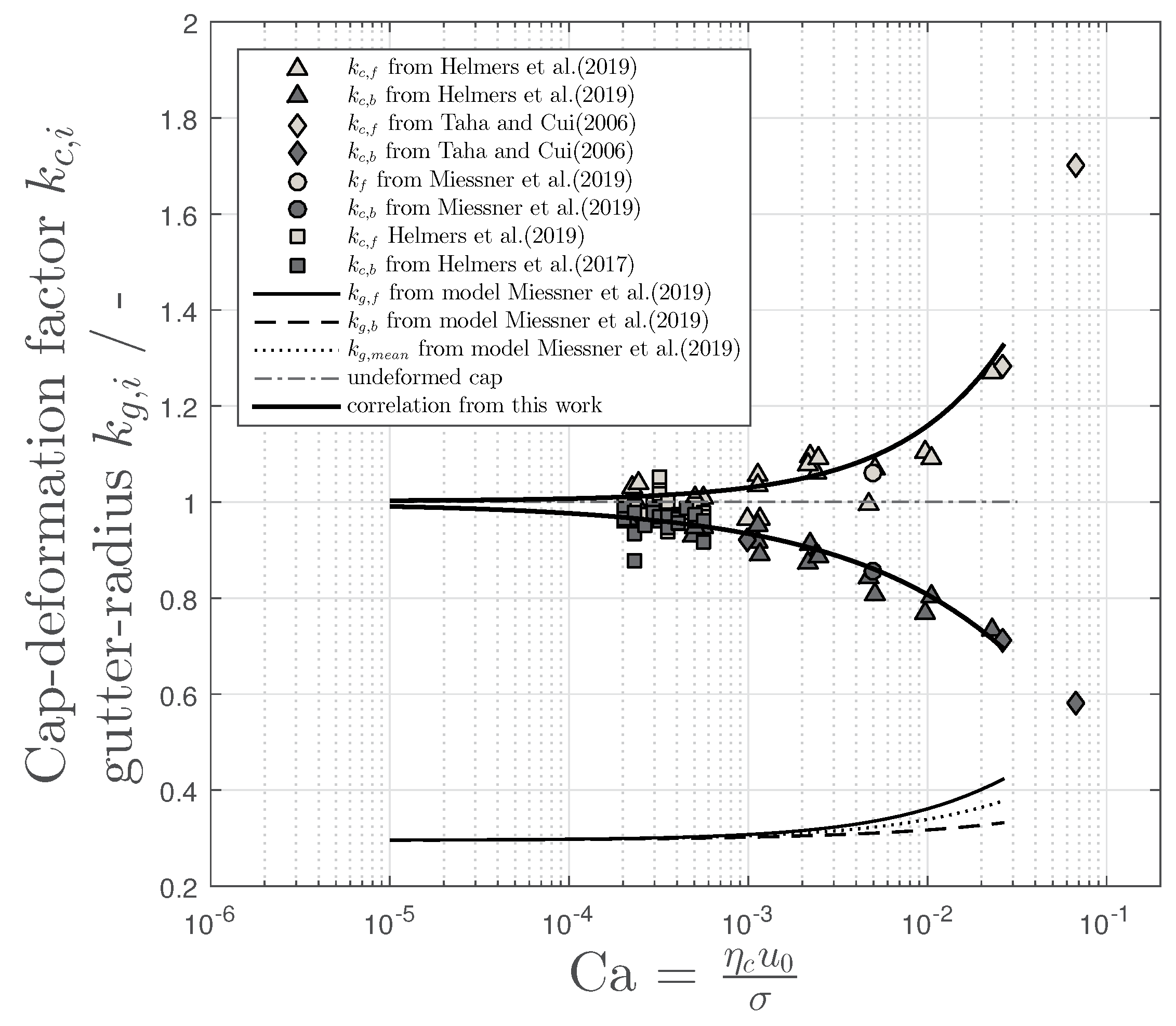
In previous work [
25], we introduced a quantification of the droplet cap deformation with an elliptic approximation of the cap outline
The ratio of the semi-major
a and semi-minor axis
b of the droplet cap curvature is introduced as deformation ratios
at the droplet front and back. They become
when describing the static circular droplet cap shape of the droplet front and back. For the dynamic cap shape, under the influence of the moving liquids, the droplet front appears elongated
and the back cap is compressed in flow direction
. Hence, we introduce a correlation to describe these relations: The cap curvature only depends on the
number for moderate flows (
):
With the correlation approach from our recent publication and the model from Mießner et al. [
24], we are able to calculate the Laplace pressure at the gutters. We assume a linear connection between the gutter front and the back of the droplet body, since the curvature of the gutter in flow direction is negligibly small. In this case, the mean interface curvature at the gutter entrance and its exit depends on the gutter radii only, and the flow-induced Laplace pressure difference equals:
Those deformation related pressures at the droplet front and back provide a link to the driving pressure difference
along the gutter length in the flow direction. Due to symmetry, the static terms cancel out:
Using the dimensionless expression from Equation (
20), this results in
for the flow-induced pressure difference as a driving force.
The relative volume flow rate through the four gutters
can be modeled as a laminar pressure driven flow [
46] and it is linked to this pressure difference with a hydrodynamic resistance
:
The hydrodynamic resistance
was defined by Ransohoff and Radke [
47] and Shams et al. [
27] as
Besides the gutter length
,
denotes a dimensionless factor, which represents the geometrical obstructions of the gutter flow, as well as the viscous coupling of both flow phases. In accordance with the simulation results of Shams et al. [
27], we declare an influence from the viscosity ratio
of the flow phases to take care of the viscous coupling effects:
The gutter length
can be derived from the droplet length
, if the gutter distance
from the caps is subtracted:
The gutter distance from the front and back droplet tip
was defined by Mießner et al. [
24] as
The above-stated considerations lead to our final description for the relative volume flow through the gutters
Herein,
and
depend on
as the preceding considerations show. Thus,
has the most prominent influence feature besides
. Inserting Equations (
36) and (
33) into Equation (
19) delivers
expanding with
and inserting
(Equation (
34)), we receive our final expression for the excess velocity:
We point out that our model is usable within the capillary regime
since the model for the wall film-thickness from Han and Shikazono [
40], the analytic interface model from Mießner et al. [
24] and the droplet curvature correlation from our recent work [
25] are valid in this range. At higher
in the viscous regime, different flow conditions with thicker wall films [
22] as well as a higher influence of
are reported [
48].
5. Model Calibration
The final expression for the excess velocity (Equation (
38)) depends on accessible data such as
W,
and
as well as on
,
,
,
,
and
, whereas the latter is also related to the gutter radii
. As shown in the previous section, the parameters can be calculated from the droplet cap curvatures
and
and via measurement-based model calibration. The six parameters (
,
,
,
,
, and
) influencing the cap deformation at the droplet front and back as well as the dimensionless resistance factor
with
and
need to be adjusted.
For model calibration, we used the dataset presented in [
25] in combination with supplementary measurements in the data range of low
and redefine
within an interval around 1. Nevertheless, for
, it represents the point of minimal surface energy and equates a spherical droplet shape. This approach allows improving the convergence of solvers. Out of further a priori considerations (
,
), we additionally defined the boundaries for the search space of the solver presented in
Table 1 and allowed the solver to adapt the correlation coefficients from our last work to the presented model and acquired measurement data.
Besides the fixed boundaries of the search space, a hydrodynamic boundary condition was applied to improve the convergence of the used optimization algorithms. For a rising
, the difference between
and
must increase, because of the pressure difference between the droplet front and back increases with higher
[
21] and the droplet front elongates, which leads to a larger front gutter radius, while the droplet rear flattens out. This is expressed by the gutter radius increase for an increasing
:
The large number of influence parameters leads to a highly nonlinear optimization problem with numerous local minima. Thus, most gradient-based algorithms are not suitable for this type of optimization problem, which tend to converge to local optima. This would result in an enormous number of randomly initialized solver calls to cover the whole search space. In contrast, stochastic and metaheuristic approaches cover the search space to solve the statistical part of the greybox model by finding the global optimum.
The quality of a solver result (e.g., deviation between measured data and estimation) is quantified by the loss-function of the problem. For the model calibration, we define
with the weights of the individual properties
,
,
following
Table 2. Values with an upper index
denote values estimated by the model and values without an upper index represent the calibration data. The first two sums serve as calibration datasets for the hydrodynamic flow properties, since they contain the flow related deformation and therefore the hydrodynamic influences. The differences of the velocity
serves as a parameter for the actual droplet velocity and therefore the flow resistance
. This is necessary, since otherwise no representation for
is available.
In addition, the concept of an equilibrium function
is introduced to maintain the overall integrity of the model: The excess velocity depends on extrinsic measurable values such as the dimensionless quantities and geometrical properties as well as varying flow properties such as the gutter length. Thus, it is appropriate to separate the measurable quantities from the model based quantities. In doing so, one can directly compare the quantities received from our correlation with measurement data adjusted for material and flow properties. The separation of those terms leads to the equilibrium function
(Equations (
41) and (42)). Herein, Equation (
41) represents the data from our measurements and Equation (42) only data from our modeling assumptions and geometry. For a well-adjusted model, the measured data for
(Equation (
41)) should systematically correspond with the modeled values for
(Equation (42)).
The calibration procedure is based on a Genetic Algorithm (GA). For good optimization results, it is necessary to emulate a sufficiently sized genome pool, thus a high number of emulated individuals is preferred. This in turn results in a massively increased calculation demand, because, for each iteration step, every single individual and their children need to be evaluated [
49]. Additionally, the genetic algorithm is typically performed iteratively to identify local optima. To decrease the number of time-consuming iteration steps of the GA and thereby reduce overall calculation time, we utilize a three-step stochastic and gradient-free approach.
In the first step, a random population at the feasible borders of the problem is generated for the Genetic Algorithm and a genetic optimization performed. The convergence point of the GA is initialized via Latin Hypercube Sampling processed by a following fast-converging Pattern Search Algorithm (PSA) [
50] that results in an improved minimum as the final convergence point. The properties of both algorithms are shown in
Table 3. The algorithm finally merges at the values shown in
Table 4. The results are discussed in the following.
For the flow-induced cap curvature, the solver merges to an exponential behavior as a function of the
number for both cap deformation ratios
and
, which coincides with the results of our previous works [
24,
25,
51]. The retrieved correlation with underlying data points is shown in the
Appendix (
Figure A2). Our additional boundary condition (Equation (
39)) is satisfied for all values as the graphs for the gutter radii
show.
For the resistance factor
, no fitting data are available since it cannot be measured directly. Therefore,
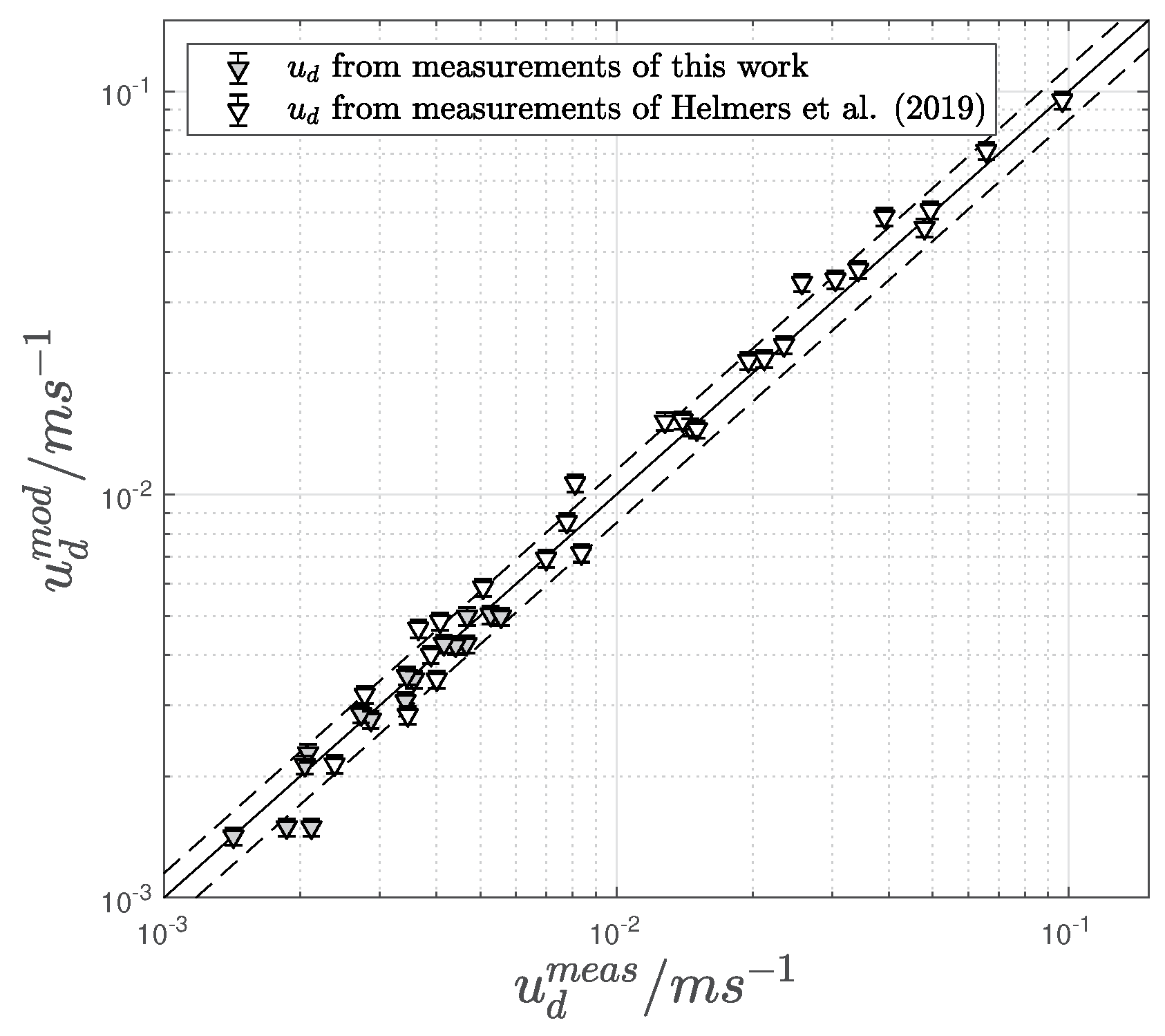
is fitted based on the velocity data from high-speed camera measurements and the application of parameters for the droplet deformation (measurements are performed in the experimental setup described in [
25]). The resulting droplet velocities in comparison with the measured values are shown in
Figure 4. The measurements fit reasonably well in the range of inevitable velocity fluctuations caused by Taylor flow stability of ±10 % range described by [
13].
6. Model Validation
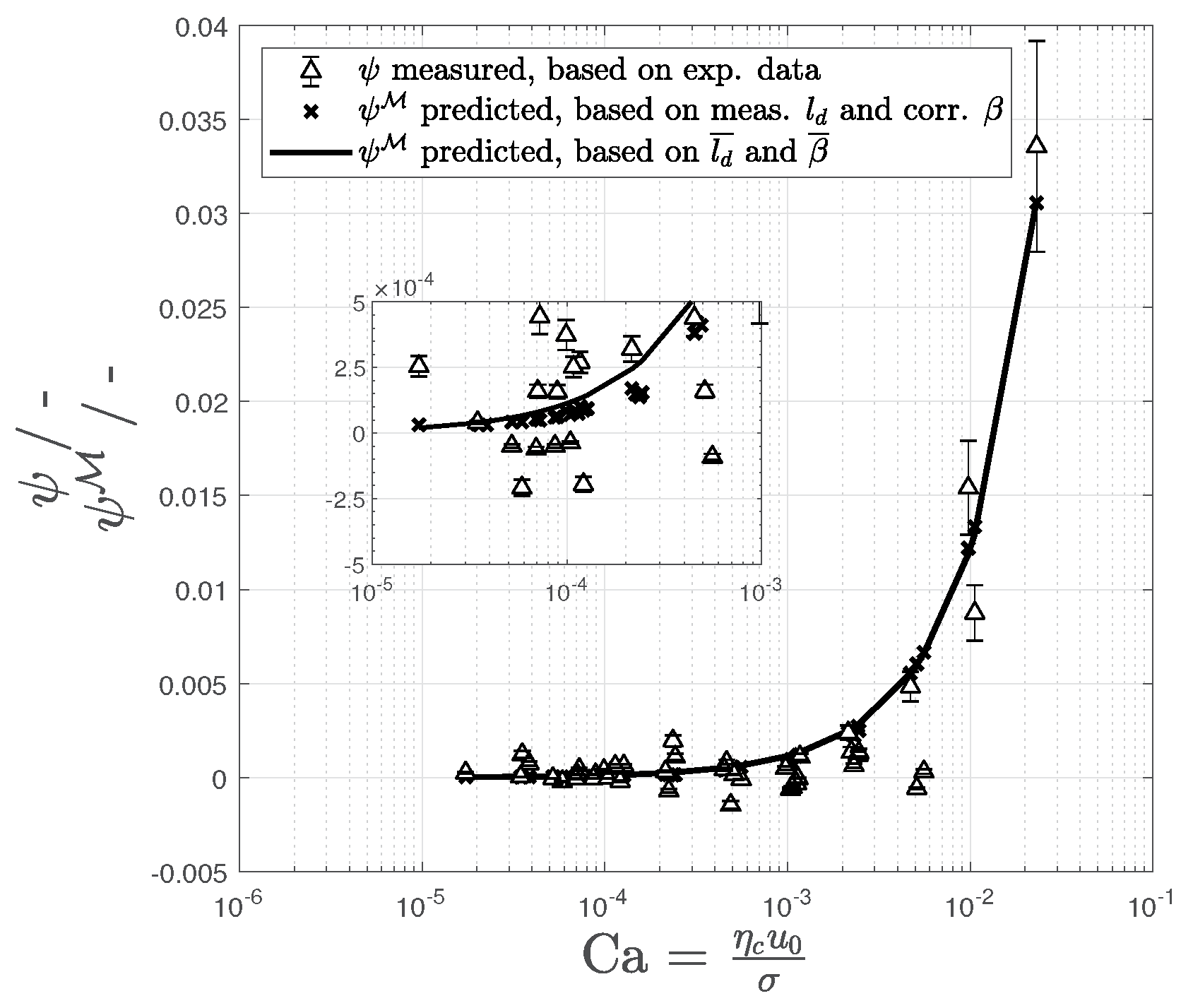
For a first validation step, the equilibrium functions
and
are considered. In the case of a hydrodynamic well-adjusted model, both functions should coincide, and our model based shape deviations (
) equal the combination of measured properties (
). The corresponding data and the values for our model agree well at high
numbers (
Figure 5), whereas a deviation for lower
numbers can be observed. This can be explained by the fact that the excess velocity itself is a relative quantity and it is strongly influenced at lower absolute values (low
number). Thus, an inevitable constant measurement deviation for velocity and volume flows caused by the experimental equipment results in a higher error for low excess velocities. Especially for
, the resulting volume flows are situated at
L/min and even minor deviations lead to high errors for the excess velocity. Thus, we consider our model approach to represent the measurements reasonably well and our fit coefficients to be valid.
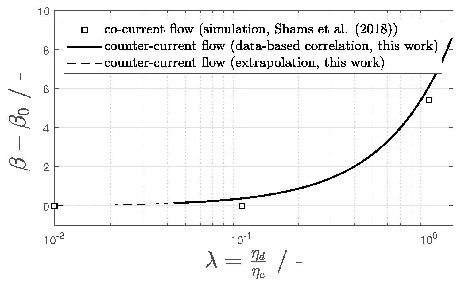
Besides the hydrodynamic validation, our assumptions for
are compared with available simulation data. We found a dependence of the gutter flow resistance
on the viscosity ratio
. The latter can be interpreted as an indicator for the viscous coupling of both flow phases (
Figure 6). In the case of a highly viscous continuous phase (
), the strongest velocity gradients are found inside the droplet, while, for a viscous disperse phase (
), larger velocity gradients and therefore energy dissipation are found inside the gutter-flow, resulting in a larger
.
This approach agrees with the simulations from Shams et al. [
27], who improved the model of Ransohoff and Radke [
47] by introducing the viscous coupling of the disperse and the continuous phase. For our case of
and a contact angle
°, Shams et al. [
27] reported a
of 20–30 for a co-current flow. Our values are shifted by a constant offset, while the slope and therefore the dependence on
is similar. We consider the difference in the offset to be caused by the use of a different flow field specifications. Shams et al. [
27] described a concurrent flow in a fixed frame specification, while in this work we determine
within a moving frame flow specification. The coordinate transformation only changes the offset of the function, while the hydrodynamic influence (the slope) must remain identical. Additionally, within the simulation of [
27], they assumed a contact line between disperse phase, continuous phase and the wall in their problem definition. Although for the solution shown in
Figure 6 the contact angle for the continuous phase is nearly 180°, the existence of a contact line introduces an additional resistance. Thus, regarding
, we consider our model plausible.
Due to the mentioned experimental restrictions, we cannot directly compare the modeled and experimental determined excess velocities
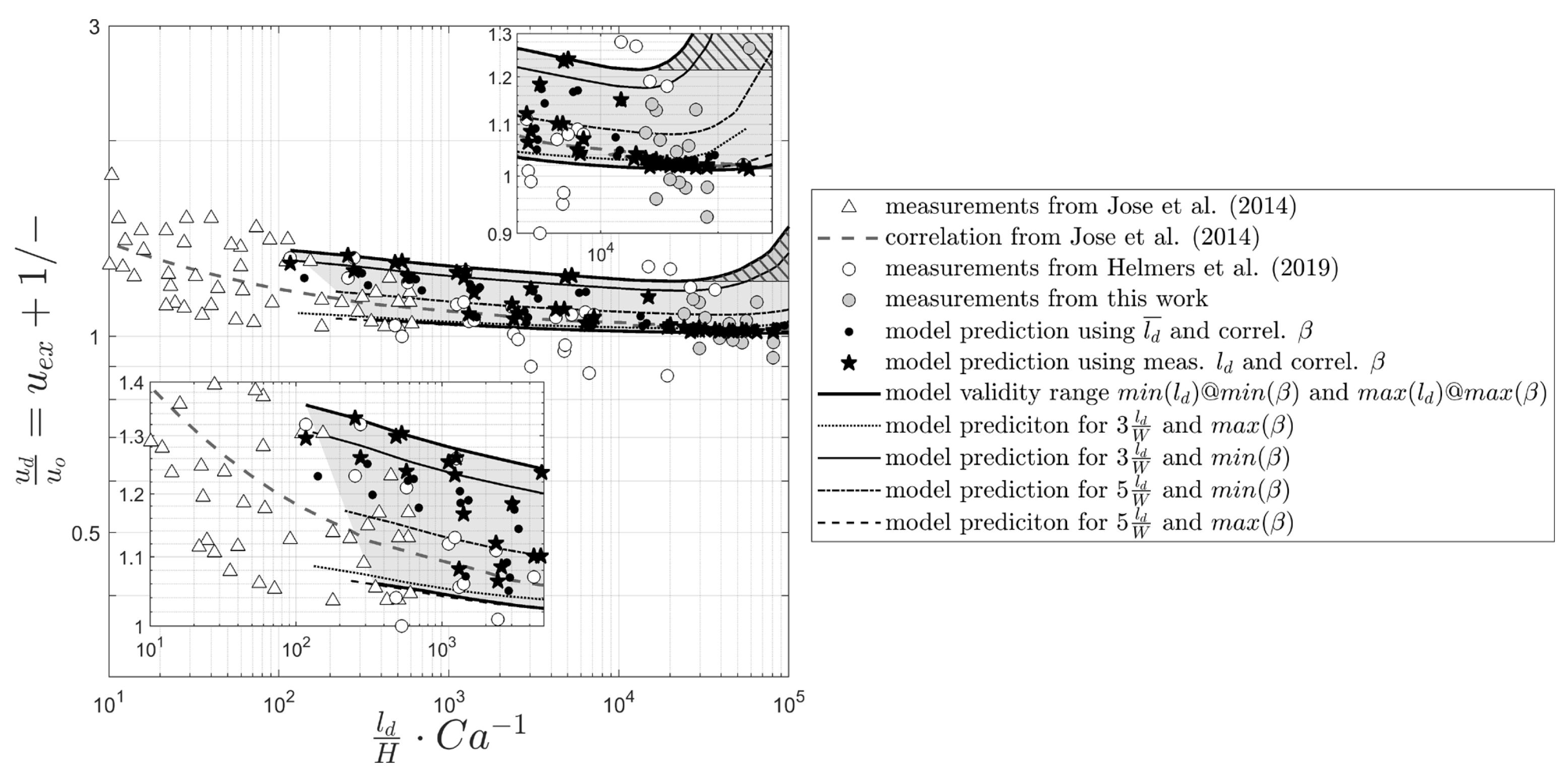
. Instead, we compared the results of our model to different published approaches. A suitable correlation for the prediction of the excess velocity in the first regime was introduced by Jose and Cubaud [
22], who identified the
number and the ratio of the droplet length
as characteristic properties (
Figure 7). It has to be mentioned that the model of Jose and Cubaud [
22] for non-wetting droplets ends at
, since for larger values they observed the disperse phase to wet the channel walls. This results in intensified dissipation and a higher pressure drop and thereby inhibits a gutter flow from the droplet front to the back. This phenomenologically equals the second flow regime, as mentioned by Wong et al. [
5], but lacks the thin wall film and results in a much larger pressure drop. Furthermore, the viscosity ratio
is not included in their correlation.
A comparison of our greybox model with the correlation from Jose and Cubaud [
22] (
Figure 7) shows good agreement. At very low
numbers (
), our model results in a slightly increased excess velocity. We regard this behavior of the model as not physical. The effect results from the mathematical counterplay of the terms
within Equation (
38). To achieve a stable solver convergence, we accepted a small residual deviation for the static case
for the front and back shape of
. Due to the relative character of the excess velocity, this unfolds a significant influence at low
values. Unfortunately, additional measurement validation concerning the shape deviation at very low
is not possible in our experimental design, since the expected shape deviation is smaller than the blurriness of the interfacial area in the images itself and therefore lies inside the measurement deviation.
7. Discussion
The interfacial area of a Taylor droplet in rectangular channels can be divided into the front and back cap regions, the wall films and the gutter interface. Neglecting the caps, the main momentum input into a droplet is transferred across the wall film and the gutter interface area. An increasing channel aspect ratio and droplet length result in a growing wall film area, i.e., an enlarged dissipation interface.
As shown in
Section 2, the behavior of the Taylor droplet’s excess velocity can be parted in two possible regimes and the viscosity ratio
has a strong influence on the hydrodynamic mechanisms. In the first regime, the fluid in the gutter flows slower than the droplet, exerting a drag force and leading to a positive excess velocity
. These drag forces influence the droplet shape, leading to a flattened droplet back and elongated droplet front. We characterize this shape variation with a correlation (
Section 5). As can be seen from the measurements, our data fall into this flow regime, as our resulting droplet shape indicates in accordance with Wong et al. [
29].
The influence of the droplet length in the plug flow regime and
, where larger droplets have an
, is in agreement with Jakiela et al. [
31] and their later publication [
53]. Additionally, they found an elongation of the dynamic droplet length in comparison to the static droplet length, which is also covered by our shape correlation, since for rising the
number the droplet front elongates stronger than the droplet back is compressed. Recently published simulations by Kumari et al. [
54] show that also for larger
numbers
.
Our concept of deriving the excess velocity from the gutter pressure drop that is directed against the flow direction (larger pressure at the front gutter entrance) is in accordance with Abiev [
21]. Nevertheless, the averaged pressure is still higher at the droplet back than at the droplet front due to the overall droplet pressure drop, since the droplet needs a driving force for its translation.
For the second flow regime identified by Wong et al. [
29], where the viscous dissipation in the film and droplet leads to a bypass flow from the droplet back to the front and therefore a negative droplet excess velocity (for large
and long droplets), our model can be adapted, if the gutter-shape-difference term is revised or a resistance coefficient for the film is added. As the viscosity ratio
rises, more momentum will be dissipated via the wall films. This extra momentum is dissipated at the gutter interface, which results in a slower droplet velocity, forcing the continuous phase to bypass the droplet reversely. As the hydrophilized channels walls in our experimental setup did not allow establishing a water-in-oil two-phase flow with a
, droplet shape correlations, as well as measurements of
for the case of
should be performed in future work. Although we assume a systematic inversion of the gutter radii ratio back to front as a consequence of the reversed gutter flow direction, it should be mentioned that, with the current shape correlation, our model only works for the case of low viscous disperse phase (
) such as gas/liquid or low viscous oil/water flows.
The influence of the channel aspect ratio, as mentioned by Wong et al. [
5], is incorporated in our model: a higher aspect ratio results in lower excess velocities. This can be explained by the larger drag forces acting on a larger relative wall film area caused by the flattened channel geometry.
8. Conclusions
In this work, we developed a model to determine the relative droplet velocity of Taylor flows in square microchannels for moderate numbers and low to moderate viscosity disperse phase (). We base our model on the relative volume flow through the gutters, as well as the wall film-thickness. The flow through the gutters is determined from the pressure drop described by the Laplace pressure difference between the gutter entrances.
Our model uses the gutter radii to obtain the resulting pressure gradient that drives the continuous phase through the gutters. We used measurements at different
and
in a surfactant-free fluid system from a previous publication [
25] to derive the radii at the gutter entrances from the surface shape model proposed by Mießner et al. [
24] and calibrate the model parameters.
Our model was successfully validated with an intrinsic approach comparing the congruence of measurement data and calibrated model parameters. Additionally, we successfully compared our model to the phenomenological correlation of Jose and Cubaud [
22].
The comparison with the most prominent approaches shows that our model and the chosen influential parameters are valid for moderate and small viscosity ratios. The excess velocity is determined by viscous dissipation in the droplet and the gutters as well as the drag of the thin wall films. The relation is characterized by the number, the viscosity-ratio , the dimensionless gutter-length , the aspect ratio and the wall film area . Furthermore, the proposed model can close the gap for and allows the calculation of the excess velocity for moderate numbers ().
In the future, the influence of surfactants and highly viscous droplets () on the excess velocity should be investigated to extend the model, since an excess velocity has not been included into the model so far. We suggest to include this function in the modeling of the wall film resistance. Especially local spatially resolved measurement techniques, e.g., µPIV measurements, should be appropriate for this task.


